3D Hydrodynamic Simulations of Relativistic Extragalactic Jets

Abstract

We describe a new numerical 3D relativistic hydrodynamical code and present the results of three validation tests. A comparison of an axisymmetric jet simulation using the 3D code, with corresponding results from an earlier 2D code, reveal that a) the enforcement of axisymmetry in the 2D case had no significant influence on the global morphology and dynamics; b) although 3D studies typically have lower resolution than those using 2D, limiting their ability to fully capture internal jet structure, such 3D studies can provide a reliable model of global morphology and dynamics.

The 3D code has been used to study the deflection and precession of relativistic flows. We find that even quite fast jets ($\gamma\sim 10$) can be significantly influenced by impinging on an oblique density gradient, exhibiting a rotation of the Mach disk in the jet’s head. The flow is bent via a potentially strong, oblique internal shock that arises due to asymmetric perturbation of the flow by its cocoon. In extreme cases this cocoon can form a marginally relativistic flow orthogonal to the jet, leading to large scale dynamics quite unlike that normally associated with astrophysical jets. Exploration of a $\gamma=5$ flow subject to a large amplitude precession (semi-angle $11\fdg 25$) shows that it retains its integrity, with modest reduction in Lorentz factor and momentum flux, for almost $50$ jet-radii, but thereafter, the collimated flow is disrupted. The flow is approximately ballistic, with velocity vectors not aligned with the local jet ‘wall’. However, sufficiently large changes in flow direction take place within the jet that for observers close to the jet axis, significant changes in Doppler boost would be evident along the flow.

We consider simple estimators of the flow emissivity in each case and conclude that a) while the oblique internal shocks which mediate a small change in the direction of the deflected flows have little impact on the global dynamics, significantly enhanced flow emission (by a factor of $2-3$) may be associated with such regions; and b) the convolution of rest frame emissivity and Doppler boost in the case of the precessed jet invariably leads to a core-jet-like structure, but that intensity fluctuations in the jet cannot be uniquely associated with either change in internal conditions or Doppler boost alone, but in general are a combination of both factors.

1 Introduction

Collimated extragalactic flows, exhibiting a complex pattern of internal structures, often with high brightness temperature and/or superluminal speed, have been explored with increasing spatial and temporal resolution over the last two decades (Zensus, 1997). Remarkably, it has become evident over the last five years that the highly energetic flows associated with active galactic nuclei are also found in Galactic objects with stellar mass ‘engines’. In the galactic superluminals GRS 1915+105 (Mirabel and Rodríguez, 1994, 1995) and GRO J1655–40 (Hjellming and Rupen, 1995; Tingay et al., 1995) the observed motions indicate jet flow speeds up to $0.98c$. Further, there is compelling evidence from the observation of optical afterglow that gamma-ray bursts are of cosmological origin, and whether produced by the mergers of compact objects, or accretion induced collapse (AIC), simple relativistic fireball models seem ruled out, the data strongly favoring highly relativistic jets (Dar, 1998). Thus a detailed understanding of the dynamics of collimated relativistic flows has wide application in astrophysics.

A particularly important facet of these flows has been revealed over the last decade as the quantity and quality of images of extragalactic relativistic jets have increased: the curvature of parsec-scale flows is the norm, not the exception; see e.g., Wardle et al. (1994). Some of this curvature may be ‘apparent’, resulting from a more modestly curved flow seen close to the line of sight. Nevertheless, such flows must posses intrinsic curvature, and we are forced to ask how such highly relativistic flows can exhibit significant curvature, and yet retain their integrity, transporting energy and momentum efficiently to the kiloparsec scale and beyond. Indeed, the structure (large-scale curvature, sheaths and filaments, and ‘knots’ of emission) of such flows provides a powerful diagnostic tool, that may elucidate the intrinsic instability, precession, deflecting obstacles and cross-winds to which the flow is subjected (although it is important to note that the mere presence of structure cannot uniquely determine its origin: at a minimum we must explore the velocity and magnetic fields of such features, and their evolution).

Numerous lines of evidence point convincingly to the occurrence of both transverse and oblique shocks, e.g., (Heinz and Begelman, 1997; Lister et al., 1998; Marscher et al., 1997; Polatidis and Wilkinson, 1998) in such flows; how do they form and evolve? Specifically, how do transverse shocks propagate along a curved flow; will the shock plane rotate with respect to the flow axis; will the shock strengthen or weaken? What role does flow curvature have to play in explaining phenomena such as stationary knots between which superluminal components propagate (Shaffer et al., 1987), knots which brighten after an initial fading (Mutel et al., 1990), and changing component speed (Lobanov and Zensus, 1996). All these issues are potentially important in both the extragalactic and stellar jet contexts, and are amenable to study through hydrodynamic simulation – but all demand that such simulations be 3D.

Numerical hydrodynamical studies of relativistic astrophysical jets have been available for barely five years. Wilson (1987) and Bowman (1994) explored steady relativistic jets, but it was only with the advent of robust, shock-capturing 2D schemes (van Putten, 1993, 1996; Duncan and Hughes, 1994; Martí, et al., 1994, 1995, 1997; Komissarov and Falle, 1998; Rosen et al., 1999) that a full exploration of relativistic flows began. Koide et al. (1996), Nichikawa et al. (1997) and Nichikawa et al. (1998) have pioneered 3D MHD studies where fluid is injected into a strong, ordered magnetic field, but the detailed structure and evolution of 3D flows remains largely unexplored (Aloy et al., 1999). The current paper describes extension of our original 2D code (Duncan and Hughes, 1994) to 3D, and its first application to axisymmetric, deflected and precessed flows. Our immediate goals are to study: the internal structures that arise from the development of Kelvin-Helmholtz instability, which may explain features such as those seen in the jet of M 87 (e.g., components E and A (Perlman et al., 1999)); the formation of oblique shocks which may mediate a change in flow direction (e.g., 1127$-$-145 and CTA 102 (Jorstad et al., 2001)); and precession which may underly the evolving, approximately helical trajectories exhibited by a number of parsec-scale flows (e.g., BL Lac (Denn, Mutel and Marscher, 1999)).

2 Numerical Solver for the Euler Equations

We assume an inviscid and compressible gas, and an ideal equation of state with constant adiabatic index. We use a Godunov-type solver which is a relativistic generalization of the method due to Harten et al. (1983), and Einfeldt (1988), in which the full solution to the Riemann problem is approximated by two waves separated by a piecewise constant state. We evolve mass density $R$, the three components of the momentum density $M_{x}$, $M_{y}$ and $M_{z}$, and the total energy density $E$ relative to the laboratory frame.

Defining the vector (in terms of its transpose for compactness)

$$U=(R,M_{x},M_{y},M_{z},E)^{T},$$ (1)

and the three flux vectors

$$F^{x}=(Rv^{x},M_{x}v^{x}+p,M_{y}v^{y},M_{z}v^{z},(E+p)v^{x})^{T},$$ (2)

$$F^{y}=(Rv^{y},M_{x}v^{x},M_{y}v^{y}+p,M_{z}v^{z},(E+p)v^{y})^{T},$$ (3)

$$F^{z}=(Rv^{z},M_{x}v^{x},M_{y}v^{y},M_{z}v^{z}+p,(E+p)v^{z})^{T},$$ (4)

the conservative form of the relativistic Euler equation is

$${\partial{U}\over\partial{t}}+{\partial\over\partial{x}}(F^{x})+{\partial\over\partial y}(F^{y})+{\partial\over\partial z}(F^{z})=0.$$ (5)

The pressure is given by the ideal gas equation of state $p=(\Gamma-1)(e-n).$ The Godunov-type solvers are well known for their capability as robust, conservative flow solvers with excellent shock capturing features. In this family of solvers one reduces the problem of updating the components of the vector $U$, averaged over a cell, to the computation of fluxes at the cell interfaces. In one spatial dimension the part of the update due to advection of the vector $U$ may be written as

$${U^{n+1}}_{i}={U^{n}}_{i}-\frac{\delta t}{\delta x}(F_{i+\frac{1}{2}}-F_{i-\frac{1}{2}}).$$ (6)

In the scheme originally devised by Godunov (1959), a fundamental emphasis is placed on the strategy of decomposing the problem into many local Riemann problems, one for each pair of values of $U_{i}$ and $U_{i+1}$, to yield values which allow the computation of the local interface fluxes $F_{i+\frac{1}{2}}$. In general, an initial discontinuity at $i+\frac{1}{2}$ due to $U_{i}$ and $U_{i+1}$ will evolve into four piecewise constant states separated by three waves. The left-most and right-most waves may be either shocks or rarefaction waves, while the middle wave is always a contact discontinuity. The determination of these four piecewise constant states can, in general, be achieved only by iteratively solving nonlinear equations. Thus the computation of the fluxes necessitates a step which can be computationally expensive. For this reason much attention has been given to approximate, but sufficiently accurate, techniques. One notable method is that due to Harten et al. (1983, HLL), in which the middle wave, and the two constant states that it separates, are replaced by a single piecewise constant state. One benefit of this approximation, which smears the contact discontinuity somewhat, is to eliminate the iterative step, thus significantly improving efficiency. However, the HLL method requires accurate estimates of the wave speeds for the left- and right-moving waves. Einfeldt (1988) analyzed the HLL method and found good estimates for the wave speeds. The resulting method combining the original HLL method with Einfeldt’s improvements (the HLLE method), has been taken as a starting point for our simulations. In our implementation we use wave speed estimates based on a simple application of the relativistic addition of velocities formula for the individual components of the velocities, and the relativistic sound speed $c_{s}$, assuming that the waves can be decomposed into components moving perpendicular to the three coordinate directions.

In order to compute the pressure $p$ and sound speed $c_{s}$ we need the rest frame mass density $n$ and energy density $e$. However, these quantities are nonlinearly coupled to the components of the velocity as well as to the laboratory frame variables via the Lorentz transformation:

$$R=\gamma n,$$ (7)

$$M^{x}=\gamma^{2}(e+p)v^{x},$$ (8)

$$M^{y}=\gamma^{2}(e+p)v^{y},$$ (9)

$$M^{z}=\gamma^{2}(e+p)v^{z},$$ (10)

$$E=\gamma^{2}(e+p)-p,$$ (11)

where $\gamma=(1-v^{2})^{-1/2}$ is the Lorentz factor and $v^{2}=(v^{x})^{2}+(v^{y})^{2}+(v^{z})^{2}$. When the adiabatic index is constant it is possible to reduce the computation of $n$, $e$, $v^{x}$, $v^{y}$ and $v^{z}$ to the solution of the following quartic equation:

$$\Bigl{[}\Gamma v\left(E-Mv\right)-M\left(1-v^{2}\right)\Bigr{]}^{2}$$

$$-\left(1-v^{2}\right)v^{2}\left(\Gamma-1\right)^{2}R^{2}=0,$$ (12)

where $M^{2}=(M^{x})^{2}+(M^{y})^{2}+(M^{z})^{2}$. This quartic is solved at each cell several times during the update of a given mesh using Newton-Raphson iteration.

Our scheme is generally of second order accuracy, which is achieved by taking the state variables as piecewise linear in each cell, and computing fluxes at the half-time step. However, in estimating the laboratory frame values on each cell boundary, it is possible that through discretization, the laboratory frame quantities are unphysical – they correspond to rest frame values $v>1$ or $p<0$. At each point where a transformation is needed, we check that the conditions $M/E<1$ and $R/E<\left[1-\left(M/E\right)^{2}\right]^{1/2}$ are satisfied, and if not, recompute cell interface values in the piecewise constant approximation. We find that such ‘fall back to first order’ rarely occurs.

3 Adaptive Mesh Refinement

The relativistic HLLE (RHLLE) method constitutes the basic flow integration scheme on a single mesh. We use adaptive mesh refinement (AMR) in order to gain spatial and temporal resolution for given computer resources.

The AMR algorithm used is a general purpose mesh refinement scheme which is an outgrowth of original work by Berger (1982) and Berger and Colella (1989). The AMR method uses a hierarchical collection of grids consisting of embedded meshes to discretize the flow domain. We have used a scheme which subdivides the domain into logically rectangular meshes with uniform spacing in the three coordinate directions, and a fixed refinement ratio of $\times 3$. The AMR algorithm orchestrates i) the flagging of cells which need further refinement, assembling collections of such cells into meshes; ii) the construction of boundary zones so that a given mesh is a self-contained entity consisting of the interior cells and the needed boundary information; iii) mechanisms for sweeping over all levels of refinement and over each mesh in a given level to update the physical variables on each such mesh; and iv) the transfer of data between various meshes in the hierarchy, with the eventual completed update of all variables on all meshes to the same final time level. The adaption process is dynamic so that the AMR algorithm places further resolution where and when it is needed, as well as removing resolution when it is no longer required.

Adaption occurs in time, as well as in space: the time step on a refined grid is less than that on the coarser grid, by the refinement factor for the spatial dimension. More time steps are taken on finer grids, and the advance of the flow solution is synchronized by interleaving the integrations at different levels. This helps prevent any interlevel mismatches that could adversely affect the accuracy of the simulation. The time step value is computed by applying the CFL condition to every cell within the computational domain, using the relativistic sum of the local flow velocity and sound speed, and picking the globally minimum value of $dt$. The corresponding time step on the coarsest level is computed, and multiplied by a CFL number, typically $0.1$.

In order for the AMR method to sense where further refinement is needed, some monitoring function is required. We have used a combination of the gradient of the laboratory frame mass density, a test that recognizes the presence of contact surfaces, and a measure of the cell-to-cell shear in the flow, the choice of which functions to use being determined by which part of the flow is of most significance in a given study. Since the tracking of shock waves is of paramount importance, a buffer ensures the flagging of extra cells at the edge of meshes, ensuring that important flow structures do not ‘leak’ out of refined meshes during the update of the hydrodynamic solution. The combined effect of using the RHLLE single mesh solver and the AMR algorithm results in a very efficient scheme. Where the RHLLE method is unable to give adequate resolution on a single coarse mesh the AMR algorithm places more cells, resulting in an excellent overall coverage of the computational domain.

4 Code Validation

The testing of codes for both 2D and 3D numerical hydrodynamics, and the appraisal of the quality of the ‘solver’, in terms of its ability to accurately capture both the structure and location of shocks and contact surfaces is always challenging, because of the sparsity of problems with analytic solutions; this is particularly true in the case of relativistic flows. We present the results of three common tests below, but also note that the solver employed in the current code is a direct extension to 3D (with a recast from Fortran 77 to Fortran 90) of the solver described by Duncan and Hughes (1994). Evidence for the accuracy and robustness of that code comes from, in addition to its application to test problems: a) the general agreement between studies performed with that code and with independently constructed codes, e.g., that of Martí, et al. (1997); b) the agreement between simulations performed with that code and analytic estimates of the expected morphology and dynamics, e.g., Rosen et al. (1999); and c) the agreement between internal jet structures found in simulations performed with that code and the predictions of linear stability analyses (Hardee et al., 1998; Rosen et al., 1999). The primary goal of the tests presented here is to validate the extension and translation of the original 2D code, and its inclusion in a newly constructed AMR ‘harness’.

4.1 1D Relativistic Shock Tube

The initial condition for the 1D relativistic shock tube problem comprises two piecewise constant states separated by a discontinuity at the origin. The left and right states have pressure and rest density: $p_{L}=10^{4}$, $p_{R}=10.0$, $n_{L}=1.0$, and $n_{R}=0.1$. The fluid is initially at rest and the adiabatic index is taken to be $\Gamma=4/3$. For time $t>0$ a rarefaction wave propagates to the left and a contact surface and shock wave, which bound a narrow region of shocked flow, propagate to the right; the analytic solution has been provided by Thompson (1986).

The computational domain is taken to be $x,y,z=[-1.0,1.0]$. We have run the shock tube problem with the shock propagating along the $x$, $y$ and $z$ axes, in each case in ‘unigrid’ mode (a single level, high resolution grid) and with refinement by two levels of $\times 3$ each, with the base grid resolution chosen so that the resolution of the finest grid matches that of the unigrid runs. The code produces comparable results independent of the coordinate direction of the shock propagation, and – within refined regions – an adaptive solution that is as good in quality of fit to the analytic solution as is the unigrid case. (In general the unigrid and refined solutions are not identical to machine accuracy, because it is possible that in the refined case – depending on the choice of parameters that control where refinement occurs – there are sections of the computational domain that remain unrefined; such domains can lead to very small changes in the location of refined structures.) Figure 1 shows an example of the numerical and analytic solutions for the 1D shock tube tests. The left panels show, from top to bottom, the rest frame density, pressure and Lorentz factor for the whole computational domain; the right panels show in detail the structure of the flow in the vicinity of the contact/shock. The dashed line is the analytic solution.

4.2 3D Relativistic Shock Reflection

The initial condition for the 3D relativistic shock reflection problem comprises two piecewise constant states separated by a discontinuity at an arbitrary radius of 0.5. The inner and outer states have pressure and rest density: $p_{I}=1.0$, $p_{O}=4.0$, $n_{I}=1.0$, and $n_{O}=4.0$. The fluid is initially at rest and the adiabatic index is taken to be $\Gamma=4/3$. The values were chosen to permit comparison with the test run results of Wen et al. (1997) for a 1D shock-patching code. For time $t>0$ a shock propagates towards the origin, reflects, and moves outwards to interact with the contact surface between the initial states.

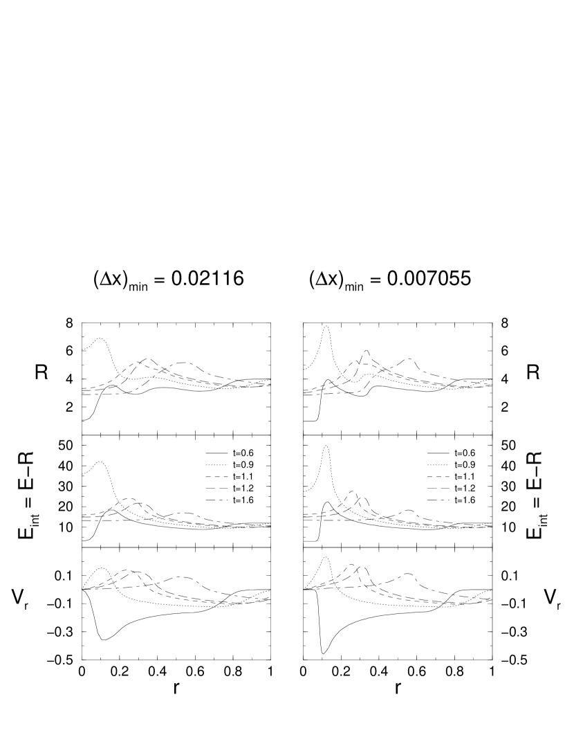
Figure 2: Cuts showing the evolution of the laboratory frame density ($R$), internal energy ($E-R={\gamma}^{2}(e+p)-p-\gamma n$) and radial velocity ($v_{r}$) for the relativistic shock reflection problem. In the left panels four levels of refinement are used, in the right five levels are used. Within each panel each line corresponds to a different elapsed time, as indicated by the line-type code in the center panels.

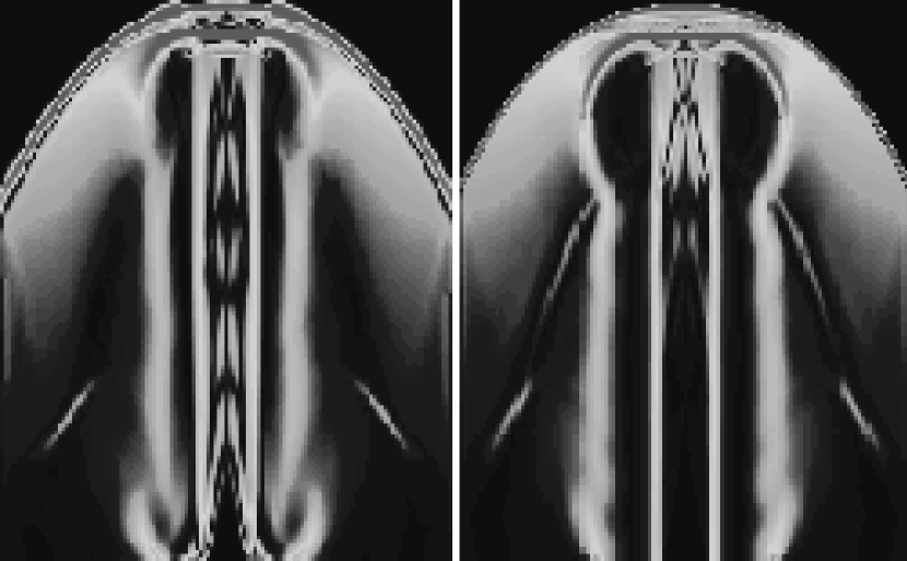
Figure 4: A schlieren plot of laboratory frame density gradient for an axisymmetric inflow with $\gamma=5.0$, ${\cal M}=8$ and $\Gamma=5/3$ after 400 cycles. Left: 3D simulation; Right: 2D simulation with the same resolution. As discussed in the text, the slight differences in wave-structure between the two simulations can be understood as due to a difference in the way the wave modes are driven, in terms of the location and amplitude of the driving perturbation, and its coupling.

The computational domain is taken to be $x=[-4.0,4.0]$, $y=[-4.0,4.0]$, and $z=[-4.0,4.0]$. The base grid (AMR level $=1$) was chosen to contain 15 points, yielding a base grid discretization scale of ${\Delta x}_{\verb+base+}=\frac{8}{14}\simeq 0.571$. Note that the discretization scale of the base grid is larger than the radius of the initial discontinuity! Figure 2 shows the evolution of the laboratory frame density $R=\gamma n$, the laboratory frame internal energy density $E_{\verb+int+}=E-R={\gamma}^{2}(e+p)-p-\gamma n$, and the $x-$component of the fluid velocity $V^{x}$ along the $x-$axis. The left panel shows the evolution of the fields with three additional levels of refinement (${\Delta x}_{\verb+fine+}=8/14/3^{3}\simeq 0.02116$), whereas the right hand panel shows the evolution of the fluid with four additional levels of refinement (${\Delta x}_{\verb+fine+}=8/14/3^{4}\simeq 0.007055$). The output times, $t=0.6,0.9,1.1,1.2$, and $1.6$, were chosen so as to easily compare with results from the $1-$D code written by Wen, Panaitescu, and Laguna (Figure 4, right panel of  Wen et al. (1997)). Although the discretization scale for the $1-$D code ($\Delta r=10^{-3}$) is almost an order of magnitude smaller than the discretization scale of the finest grid of our 3D AMR code (${\Delta x}_{\verb+fine+}=0.007055$), we find good agreement between the two. Note that the effective resolution of this simulation is 1135 x 1135 x 1135, which would require over 200 GB (GigaBytes) of memory. In contrast, our AMR code requires only 1.9 GB to run this simulation. In this case, AMR techniques have decreased the memory footprint of the simulation by two orders of magnitude!

4.3 3D Relativistic Blastwave

The 3D relativistic shock reflection problem does not exhibit highly relativistic flow speeds during the evolution covered by the simulation, and the major structures are interior to the location of the initial discontinuity at $r=0.5$. In order to validate the code for flows $\gamma>>1$ in 3D and to explore the symmetry preserving properties of the code, we have performed a 3D blastwave simulation. In this case a shell of high density and pressure propagates outward from the initial discontinuity. Coding errors and discretization effects rapidly become apparent as an asymmetric flow. Ideally we would have used the Blandford-McKee blastwave solution (Blandford and McKee, 1976) as initial data, confirming that while the shock speed remained highly relativistic the computed solution matched the analytic one. However, when using only a wedge-shaped portion of the entire sphere, of opening angle $0.2$rad, and initial energy and density that yield a shock Lorentz factor $\Gamma\sim 28.4$, and peak fluid Lorentz factor $\gamma=1/\sqrt{2}\Gamma\sim 20$, the leading structure is so narrow that even five levels of refinement (requiring $\sim 2$Gb of memory) did not adequately resolve it: the highest Lorentz factor in the initial data being $\sim 8$. It was concluded that the Blandford-McKee blastwave constitutes a problem that is too demanding to be a useful validation test unless very significant computer resources are employed.

We have thus opted to simulate the 3D-equivalent of the shock tube problem: the initial condition for the 3D relativistic blastwave problem comprises two piecewise constant states separated by a discontinuity at an arbitrary radius $r=1.0$. A numerical solution with spherical symmetry, and initial conditions that produced marginally relativistic flow speed, was presented by van Putten (1994); here we adopt an initial state the leads to higher Lorentz factors – of order those encountered in the applications discussed in the next sections. The inner and outer states have pressure and rest density: $p_{I}=10^{4}$, $p_{O}=10.0$, $n_{I}=1.0$, and $n_{O}=0.1$. The fluid is initially at rest and the adiabatic index is taken to be $\Gamma=4/3$. For time $t>0$ a spherical shock wave propagates to larger radius. Substantial Lorentz factors ($\sim 5$) are generated, and by the end of the simulation the propagating structure encompasses $\sim 35$ times the volume of the initial high pressure sphere, which is ample development for isolating asymmetries that might arise. Some asymmetry is to be expected, because the criteria used for flagging cells to be refined is applied automatically, and a combination of differences due to rounding, coupled with the clustering algorithm, leads to a non-uniform distribution of refined patches.

Taking the computational domain to be $x=[-10.0,10.0]$, $y=[-10.0,10.0]$, and $z=[-10.0,10.0]$, Figure 3 shows the final evolution (at $t=2.3967$) of a run with $3$ levels of refinement, yielding $\sim 180$ finest level cells across the blastwave diameter at the end of the computation. The two panels show laboratory frame density ($R$) and Lorentz factor ($\gamma$) for cuts along the two orthogonal coordinate directions in the plane $x=0$, plus additional cuts that bisect these two axes. The peak laboratory frame density along the diagonal cuts is $13\%$ higher than along the coordinate directions. This is associated with an oscillation in the Lorentz factor near to its peak value $\sim 5$, in the cuts that bisect the coordinate directions. The oscillation in the Lorentz factor cuts is a result of the fact that even with an effective resolution of $\sim 5.8\times 10^{6}$ cells encompassing the blastwave, the scale of the leading edge of the evolving structure is so narrow that the Lorentz factor varies from $\sim 5$ to $\sim 4$ over a scale of a couple of the finest cells. Off axis, the chance, and changing, location of cells with respect to the thin shell of high Lorentz factor leads to a small amplitude irregularity in the peak value, evident as fluctuation along the radial cut. Notice however that an inability to fully capture the extreme values encountered on the finest scale, does not in general influence the global location of major flow structures or their values away from these extremes. In particular, there is no global asymmetry.

4.4 Axisymmetric Jet Inflow

It is well-known from nonrelativistic hydrodynamic studies that the most rapidly growing modes of the Kelvin-Helmholtz instability are suppressed in 2D simulations (cf. Hardee and Clarke (1992)); only a fully 3D treatment can capture features likely to play a major role in determining internal jet structure. However, as internal flow structures thermalize only a small fraction of the flow’s bulk energy, axisymmetric simulations should provide a reliable picture of the gross morphology and dynamics of an initially axisymmetric flow. In order to test this expectation, and to learn what internal jet structures arise in the absence of externally driven perturbations in 3D, we have rerun case B of Duncan and Hughes (1994), using the 3D code. If the 2D and 3D results are similar in terms of gross morphology and dynamics, we can conclude that these attributes are insensitive to the details of small scale flow structure, and thus that a) earlier 2D results provided a valid picture of these relativistic flows on the large scale; and b) relatively low resolution 3D simulations should provide a valid picture of the overall morphology and dynamics of deflected and precessed jets.

The parameters for this simulation are (Lorentz factor) $\gamma=5.0$, (relativistic Mach number) ${\cal M}=8$, and (adiabatic index) $\Gamma=5/3$. The ambient density is $\times 10$ that of the inflowing jet rest density, and the jet and ambient medium are initially in pressure balance. We have achieved the same resolution within the jet ($24$ fine cells across the jet radius) by using $3$ levels of refinement, of $\times 3$ each. However, to avoid prohibitive memory requirements we have followed the jet for only $25$ jet-radii, as compared with $42$ jet-radii in the original 2D run, and in the 3D simulation we have used the finest grid only within $1.5$ jet-radii of the axis – thus the cocoon and bow are under-resolved. The computation was terminated as the bow shock reached the far edge of the domain.

Figure 4 shows a schlieren (gradient) rendition of the laboratory frame density after 400 computational cycles. For comparison, we show also a 2D simulation performed with the same maximum resolution as that achieved in 3D, having propagated $25$ jet-radii. In the absence of an externally applied periodic perturbation to the flow, the development of structure within the jet depends wholly on the driving of available modes by naturally occurring perturbations – in particular, pressure perturbations arising from Kelvin-Helmholtz ‘fingers’ growing at the contact surface between shocked jet and shocked ambient medium, and a pressure wave at the inflow (Hardee et al., 1998). In the original 2D simulation the contact surface exhibited instability only as the bow approached the edge of the computational domain. The poor resolution with which the contact is captured in 3D, and the shorter duration of the simulation, ensure that no manifestation of this slowly growing instability is seen, and thus that little jet structure develops as a result. However, the 3D simulation does exhibit a much stronger pressure wave at inflow than is seen in the corresponding 2D case. This is due to the radically different boundary conditions necessary in 3D: inflow is imposed on the plane $z=$constant, and involves cells cut by the jet boundary for which state variables must be established through a volume-weighted average of the internal and external values. To avoid a ‘leakage’ of jet momentum into the ambient material, fixed, initial values are used across the entire boundary plane at every time step. In the 2D simulation – above the jet inflow – conditions were chosen to be ‘extrapolated’ or ‘rigorous outflow’, but the initial conditions were not enforced for the duration of the computation. The ambient flow thus evolved to smear out the shear layer near the inflow in the 2D case, reducing the shear-induced wave in the jet.

Thus for 2D and 3D simulations of equal resolution there is stronger driving of available modes by a pressure wave at the inflow (Hardee et al., 1998) and over most of its length the 3D simulation exhibits more internal structure; the 2D simulation manifests internal structure of significant amplitude only just upstream of the Mach disk, where the development of instability in the better-resolved contact surface drives a weak pressure wave into the jet. From a measurement of the well-defined locations of pressure minima along the flow axis we estimate a wavelength for internal structure in the 3D case of $\lambda^{obs}\sim 7$ jet radii. As noted in Hardee et al. (1998), the actual jet radius is somewhat larger than the inflow radius, and thus analytic predictions based on the inflow scale slightly underestimate the wavelength of excited modes. Bearing this in mind, it is plausible to identify the mode excited in the 3D simulation as the second body mode, with $\lambda^{max}_{2}\sim 4.6$. This is consistent with the fact that the lower order modes have longer wavelength, and are oblique to the jet axis, and the oblique inlet pressure wave more easily couples to these than to higher order ones.

In global terms the 2D and 3D simulations are similar: the inclination of the leading bow shock, a well-defined Mach disk standing back from the contact surface, and a cocoon that (near to the head) spans at most $5$ jet-radii. This similarity is quantified by comparing the variation in density, pressure and Lorentz factor for cuts along the flow axis. Figure 5 shows that the global morphology differs little between the 2D and 3D cases. The only significant difference is seen in the off-axis cuts just upstream of the head, and reflects the more extensive, but lower amplitude, pressure wave-driven flow structure in the 3D case as discussed above. This has minimal influence on the global morphology because the internal structures are associated with only slight dissipation of the flow energy: the global dynamics is determined primarily by the energy and momentum flux along the jet and that is captured as well in 3D as in 2D. The similarity is even more striking in the dynamics: the average speed of advance of the bow shock is $0.648$ in the 2D case, and $0.651$ in the 3D case.

These results have an important implication. Our 3D simulations encompassing the global dynamics (jet, bow and contact) will not be able to achieve a spatial resolution necessary to capture the flow contact surface well-enough to reveal it’s instability, with the consequent driving of certain normal modes of the jet. However, in as much as it is the global dynamics of the source that is of interest, even the modest resolution 3D simulations that are currently viable do provide a valid picture. We are thus in a position to address the influence on global morphology of jet deflection through an encounter with ambient inhomogeneities, or large amplitude precession of the inflow. Note that as regards exploring the details of internal jet structure, we may study a pre-existing flow, established across the computational domain in pressure balance with a low density ambient medium, representing the cocoon established after the passage of a bow shock. Within available resources we have performed such simulations with $\sim 25$ cells across the jet diameter, confirmed that almost pure normal modes may be excited through precession-induced driving at frequencies suggested by linear stability theory, and demonstrated that linear stability theory correctly predicts jet structures even for highly nonlinear development ($\delta q\sim q$) (Hardee et al., 2001).

5 Results

5.1 Deflection by an Ambient Density Gradient

As noted in §1, oblique shocks are likely to play a major role in the understanding of evolving parsec-scale jets, and in the detailed morphology of kiloparsec-scale flows such as M 87. While models based on transverse propagating shocks have been extremely successful in explaining both the radio polarization and broadband behavior of BL Lac objects and QSOs (Hughes et al., 1989a, b; Marscher and Gear, 1985), it has become evident recently that only oblique structures are capable of providing a quantitative explanation for many features seen on a range of length scales (Bicknell and Begelman, 1996; Aller et al., 1999). Oblique shocks have been widely studied in the context of recollimated flows, e.g., (Leahy, 1991; Daly and Marscher, 1988) and for their role in mediating bends in supersonic flows, e.g., (Icke, 1991; Alberdi et al., 1999; Mendoza and Longair, 2001a, b). Such structures are stationary, but disturbances to the flow are likely to generate propagating oblique structures also. Here we explore both stationary and propagating oblique structures that arise due to a change in the jet direction.

Curvature may result from the nonlinear development of flow instability, as may internal structure, where, ultimately, modes driven by perturbations to the jet steepen to form shocks. We shall address this issue in future studies of the development of instability. Here we are concerned with flow curvature induced by an external influence, and the associated internal structure that mediates the change in flow direction. A jet flow may be bent by a cross-wind, an ambient pressure gradient, an ambient density gradient, or interaction with a discrete ambient inhomogeneity (cloud). A cross-wind will cause a large scale curvature such as seen in NAT and WAT sources (Muxlow and Garrington, 1991), and is unlikely to be the origin of subparsec-scale curvature, particularly given the implausibility of sustaining a cross wind deep within a galactic potential. An ambient pressure gradient will also cause large scale curvature and will relax unless sustained by a gravitational potential. In the latter case, the gradient is likely to be in the same sense as that in which the jet propagates from the central engine, leading to little or no curvature. We have thus opted to study the interaction of a relativistic flow with an ambient density gradient, as this seems the external influence most likely to cause flow curvature, and which can be regarded as an idealization of the interaction with a discrete cloud.

An issue with this type of study, known from the simulation of nonrelativistic jet interaction with clouds (Higgins et al., 1999), is that a nontrivial interaction occurs only for a narrow range of jet parameters. On either side of this range the momentum flux of the jet is either large enough that the cloud provides negligible hindrance to the jet flow, or so low that the jet is effectively stopped by a rigid obstacle. As the thrust of a relativistic jet increases rapidly with Lorentz factor, we explore in detail only flows with modest Lorentz factor: $\gamma<5$. The ambient density gradient has been modeled as a smooth ramp running from low density $n_{\rm low}$ to high density $n_{\rm high}$ away from the inflow, at angle $\phi$ to the inflow plane, and with ramp width $\Delta L$ measured in units of the jet inflow radius. The ambient medium is assumed to have uniform pressure distribution, implying a lower temperature in the high density region; that is consistent with the high density region modeling a condensation that has achieved pressure balance with the surrounding material after experiencing thermal instability. Indeed, observations of the ISM, e.g., Myers (1978), show that within each phase, the dispersion in density variations is of order the mean density, and the range of densities encountered within any phase spans typically less than an order of magnitude, with even smaller pressure variations. To assess the maximum likely consequence of such density variations, we consider a jump in density by one order of magnitude, over a scale of order the jet radius.

As anticipated, for ambient gradients more-or-less parallel to the inflow plane the jet material is either deflected to form a bubble of hot gas encompassed by the slightly distorted interface to the high density domain, or rapidly penetrates that interface. The relativistic nature of the flow does not lead to the formation of distinctive structures. Only interfaces that are highly inclined to a flow allow the flow to retain its integrity, and lead to the formation of distinct internal structures. In the following subsections we present results for a range of flow speeds and density gradient orientations. We have limited these studies to $\Delta L\sim 1$, as the jet will respond only weakly to more gradual gradients.

5.1.1 $\gamma=2.5$, $\phi=65\arcdeg$

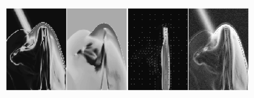
Figure 6: A slice orthogonal to the inflow plane, showing a $\gamma=2.5$ jet interacting with an oblique ($65\arcdeg$) ambient density gradient in which the density increases to the right by $\times 10$ across a region of scale length $1.2$ jet-radii. From left to right: the gradient of the laboratory frame density; the pressure; the Lorentz factor with 3-velocity vectors superposed; superposed, color-coded renditions of the left-most panel at two late epochs, showing the motion of flow features: in a monochrome render the motion of the bow and Mach disk show up as a ‘ghost’ images. The peak Lorentz factor of $2.5$ is rendered red, and values of order $1$ are dark blue – the peak values appear as the interior gray ‘stem’ in a monochrome render.

Figure 6 illustrates the case $n_{\rm low}=3$, $n_{\rm high}=30$, $\phi=65\arcdeg$ and $\Delta L=1.2$ for a jet with $n_{\rm jet}=1$ and $\gamma=2.5$. Note that a region of extremely low density and pressure and high shear (a change in $v_{z}$ by $0.94c$ over a scale $1.8$ jet-radii) develops on the low density side of the jet – immediately to the left of the inflowing jet in the left panel. The jet exhibits a number of oblique structures, primarily driven by the impact of the cocoon, the dynamics of which are clearly seen in the third panel: the cocoon is one-sided, and constitutes a structure orthogonal to the jet flow, with marginally relativistic motion partially directed towards the base of the jet. A large fraction of the low density cocoon material is moving orthogonal to, and away from, the jet with a speed $v_{x}\sim-0.396$, fast enough to exhibit (if seen face on) modest but significant Doppler boosting (by $\sim 2.25$). That part of the cocoon that impacts the ‘base’ of the jet does so with a speed $v_{x}\sim 0.34$, but the low density and small volume of this portion of the cocoon mean that the influence of this flow is only to slightly perturb the jet. Further evolution would have the jet continue to propagate within the higher density material, and the head would no longer be aware of the ambient density gradient. However, until the head is many more jet-radii further on, the shocked jet material will preferentially follow the channel that takes it back on one side of the jet, maintaining a source of driving for structures internal to the jet.

The fourth panel in Figure 6 shows a grey scale version of the first panel, colored blue, added to a reddened version of a similar snapshot 4% of the final time earlier. Unchanged regions are thus rendered neutral, while the evolved portions are evident as red or blue (or as ‘ghost’ images if seen in monochrome), and enable us to set limits on the speed of propagation of the internal jet structures; these we find to be propagating at a speed $<12\%$ of the marginally relativistic bow shock – to a good approximation they are stationary. These structures mediate a change in jet direction (by $\sim 3\fdg 5$) midway between inflow and Mach disk, which in view of the approximate stationarity of the structures must persist as the bow moves well beyond the density interface. Above the ‘bend’ the velocity component $v_{x}$ has an average sense and magnitude ($\sim-0.05c$) consistent with the entire body of the jet following the deviation in flow direction, while several jet-radii upstream of the Mach disk an oblique structure may be seen in the left-most panel of Figure 6 (crossing the jet from lower left to upper right) which is a shock in which the pressure jumps by $\sim 2.8$ and which mediates a change in the flow direction so that close to Mach disk/bow shock the flow has resumed its original direction of propagation.

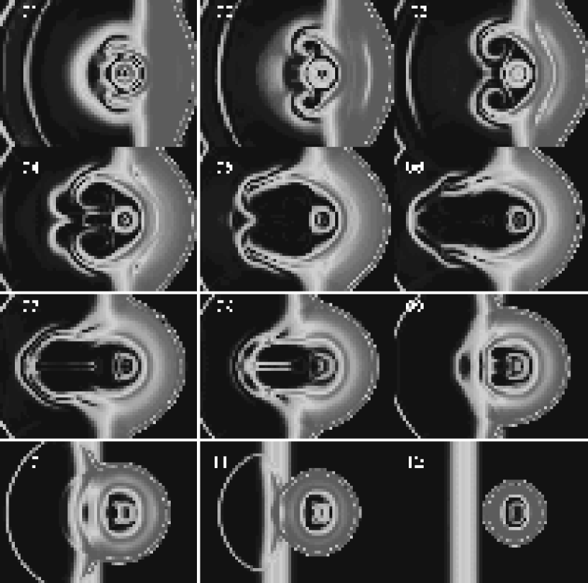
Figure 7: As for Figure 6, showing the gradient of the laboratory frame density in planes parallel to the inflow surface, at 12 equally spaced locations along the $z$-axis between the inflow plane and the Mach-disk that terminates the jet.

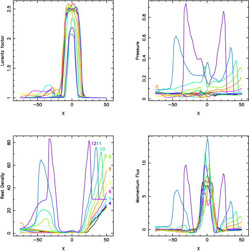
Figure 8: As for Figure 6, showing the Lorentz factor, pressure, rest frame density and momentum flux (${\cal F}=\gamma^{2}\left(e+p\right)v_{z}^{2}+p$) along the cut shown as a white line in the lower-left panel of Figure 7, at 12 equally spaced locations along the $z$-axis, between the inflow plane and the Mach-disk that terminates the jet. The numeric labels in the lower-left panel correspond to the sequence of $z$-values shown in Figure 7.

By rendering the laboratory frame density gradient in slices parallel to the inflow plane, Figure 7 shows the extent of the cocoon, also delimited by the twin-peaks in the pressure and density plots of Figure 8 which shows plots of Lorentz factor, pressure, rest frame density and momentum flux along a stack of cuts, such as the one shown by the horizontal white line in the lower-left panel of Figure 7. The upper-left panel showing the Lorentz factor makes clear the slowing of the jet just upstream of the Mach-disk, but also that the higher pressure there leads to a higher momentum flux – as seen in the lower right panel. In fact, the momentum flux increases with $z$, up to and inclusive of the 11th slice, and manifests significant variation across the cross-section of the flow at different $z$, as a consequence of the internal structure. Along a locus of peak Lorentz factor or momentum flux spanning planes $z=$constant (the result is insensitive to the choice of variable, and the locus closely follows the inflow axis) a) the Lorentz factor retains its inflow value ($2.5$) for $12$ jet radii, slowly dipping to $\sim 2$ upstream of the bow shock at $20$ jet radii; b) the momentum flux varies slowly, by less than $50$%, along the first $20$ jet radii, with a value within $10$% of its inflow value just upstream of the bow. Interaction with the ambient medium has lead to the development of discernible internal structure not seen in the axisymmetric case, but the global dynamics of the jet (if not the cocoon!) are minimally influenced by this interaction. We conclude that inhomogeneity in the ambient medium may lead to significant, oblique internal jet structure – albeit essentially stationary – with little flow energy dissipation, or change in the overall direction of the flow. Stationary VLBI structures, which may be a manifestation of such oblique shocks, are now known to be very common (Jorstad et al., 2001).

5.1.2 $\gamma=5.0$, $\phi=65\arcdeg$

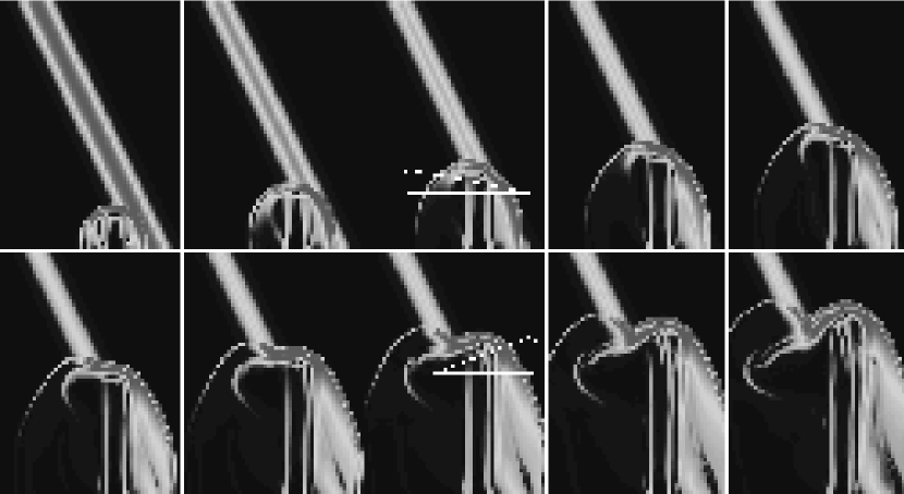
Figure 9: Slices orthogonal to the inflow plane, showing a $\gamma=5.0$ jet interacting with an oblique ($65\arcdeg$) ambient density gradient in which the density increases by $\times 10$ across a region of scale length $1.2$ jet-radii. The gradient of the laboratory frame density is rendered. Lines in the third and eighth panels indicate the sense and magnitude of the rotation of the Mach disk.

Figure 9 shows the evolution of a faster jet ($\gamma=5$) with the same inclined density gradient. The behavior is not dramatically different from that exhibited by the $\gamma=2.5$ flow, but a number of important features may be seen more clearly here. As the flow meets the density gradient, a clockwise rotation of the Mach disk occurs (upper panels in Figure 9), while after the initial interaction, the Mach disk rotates counter-clockwise (bottom panels in Figure 9) to lie orthogonal to the density incline by the last cycle of computation. The maximum clockwise rotation of the disk is $\sim 12\arcdeg$, and the maximum counter-clockwise rotation is $\sim 21\arcdeg$: highly polarized emission from the downstream flow of the Mach disk may well be the dominant feature on VLB maps, but remain unresolved, the direction of the electric vector being used to establish the likely flow direction; deviations from the transverse, by tens of degrees, could lead to a significant misestimation of the local flow direction. The jet deflection is mediated by an internal shock whose development starts to become evident in the fifth panel as a structure crossing the Mach disk. By the last cycle, this has developed to form an internal structure extending upstream from the Mach disk, with an inclination comparable to that of the density gradient. The higher momentum flux of the jet in this case ensures that deflection occurs only within the extent of this oblique shock, and the evolution is not followed far enough to see realignment of the jet along its original direction of propagation. The internal shock that moderates the jet deflection is quite strong, the rest frame density and pressure jumps being $\sim 5$ and $\sim 14$ respectively.

5.1.3 $\gamma=10.0$, $\phi=65\arcdeg$

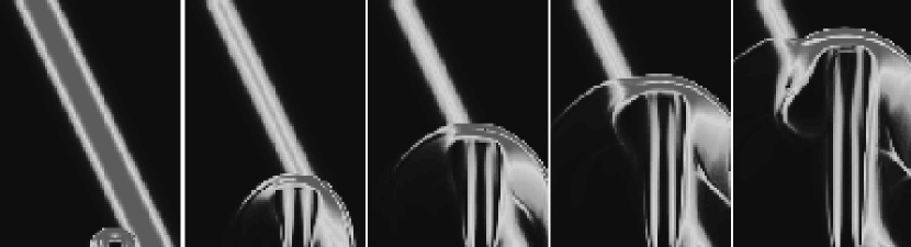
Figure 10: Slices orthogonal to the inflow plane, showing a $\gamma=10.0$ jet interacting with an oblique ($65\arcdeg$) ambient density gradient in which the density increases by $\times 10$ across a region of scale length $1.2$ jet-radii. The gradient of the laboratory frame density is rendered.

Figure 10 shows the evolution of a $\gamma=10$ jet with the same inclined density gradient. The speed and jet-to-ambient density contrast are comparable to those of cases C and D studied by Duncan and Hughes (1994) wherein it was found that the ambient medium presented little obstruction to the flow, and little internal jet structure arose. In the present case the jet head moves with high efficiency ($\sim 0.95$; see Rosen et al. (1999)) through even the densest ambient gas at relativistic speed, and all sections of the head cross the density incline before a significant rotation of the Mach disk can occur. A rotation of the Mach disk, deflection of the jet, and generation of oblique internal shocks occurs only if the jet is of low enough speed that the densest ambient regions lead to an inefficient, slow head advance there.

5.1.4 $\gamma=5.0$, $\phi=35\arcdeg$

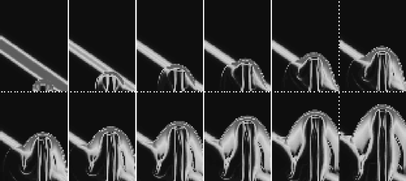
Figure 11: Slices orthogonal to the inflow plane, showing a $\gamma=5.0$ jet interacting with an oblique ($35\arcdeg$) ambient density gradient in which the density increases by $\times 10$ across a region of scale length $1.2$ jet-radii. The gradient of the laboratory frame density is rendered.

Figure 11 shows the evolution of a $\gamma=5$ jet with a density gradient inclined at a shallower angle – $35\arcdeg$ – than explored previously. As would be anticipated the clockwise/counter-clockwise rotation of the Mach disk as the jet crosses the interface is slight. However, this shallower angle case sheds light on the origin of the jet deflection. A conical pressure wave which steepens to form a weak conical shock is driven asymmetrically into the jet flow at the location of the ambient gradient, and the asymmetric nature of the flow perturbation leads to its deflection. Some jet-radii beyond this point an oblique internal shock that cuts the Mach disk returns the flow to its original direction. The inclination of the density gradient allows us to follow the jet further into the denser ambient medium in this case. By the end of the simulation both the morphology of the cocoon and the velocity field within it show that the shocked jet flow is similar – albeit still somewhat asymmetric – to that seen for propagation in a uniform environment. However, without the low density region to act as a sink for the backflowing shocked jet material, the cocoon at left, just behind the head, starts to inflate. That induces a curvature to the contact surface between shocked jet and shocked ambient material, enhanced by the Kelvin-Helmholtz instability, and this in turn drives a pressure wave into the jet just upstream of the Mach disk. A normal mode of the jet is excited (cf. Hardee et al. (1998)) which steepens to form a conical shock upstream of the Mach disk. The influence on the flow is quite significant: constriction of the flow accelerates the jet upstream of the conical shock to $\gamma\sim 6$, but the shock decelerates the flow to $\gamma\sim 4$; the corresponding pressure jump is $\sim 8.5$.

In as much as the types of interaction just discussed are uniquely associated with the leading edge of jets, the structures that result are localized, and will not form a web of propagating shocks along the length of a flow. However, this study highlights that the Mach disk associated with the hotspots of kiloparsec (and larger) scale jets may display orientations – revealed by their polarization structure – that bears no simple relation to the jet orientation and accompanied by emission from associated oblique shocks, if the head experiences a significantly inhomogeneous ambient medium. Further, on any scale, and in particular on the unresolved sub-parsec scale, a jet that restarts after a period of quiescence that allows a previously formed channel to relax, or that restarts with a new orientation, will display polarized emission that is a complex sum of that from the rotating Mach disk and developing internal shocks, and which on such scales will evolve within observable time frames.

5.2 Precession

Symmetries seen in twin-jet sources, in particular the S-symmetric sources, e.g., Leahy (1991), and the intriguing success of binary black hole models for the optical-radio waveband behavior of OJ 287, e.g., Valtonen and Lehto (1997), suggest that jets are subject to a precessional motion, and provide a quantitative explanation for the possible origin of that motion, respectively. Even if precessional motion associated with a massive binary system is not the cause of a time-dependent curvature seen in some parsec-scale flows (e.g., BL Lac; Mutel et al., private communication), an exploration of the impact of precession on flow structure and evolution will give insight into the internal structures to be found in evolving, curved flows.

As a first step in exploring the role of precession, we have applied precession to the inflow of the axisymmetric jet discussed above: a jet with inflow Lorentz factor of $5$. The inflow precesses on a cone of semi-angle $11\fdg 25$ with a frequency $0.2885$ rad measured in time units set by the inflow radius and speed. The relatively large computational domain, $\sim 32\times 32\times 82$ jet-radii, meant that we could employ only three grid levels, with refinement by $\times 3$, providing $\sim 11$ fine cells across the inflowing jet diameter. In the approximation that both the inflow speed and bow propagation speed are close to unity, the precession rate implies $\sim 3.75$ revolutions of the jet during evolution across the computational domain. The computation was terminated when the bow was $\sim 90$% of the way to the domain’s far edge, as by then significant dissipation and disruption of the jet had occurred. Renders in planes parallel to the inflow plane reveal a small influence of the boundary on structures close to the edge of the computational domain. However, there is no evidence that the limited lateral extent of the computational domain influences the spine of the flow, which is that structure of most significance to us.

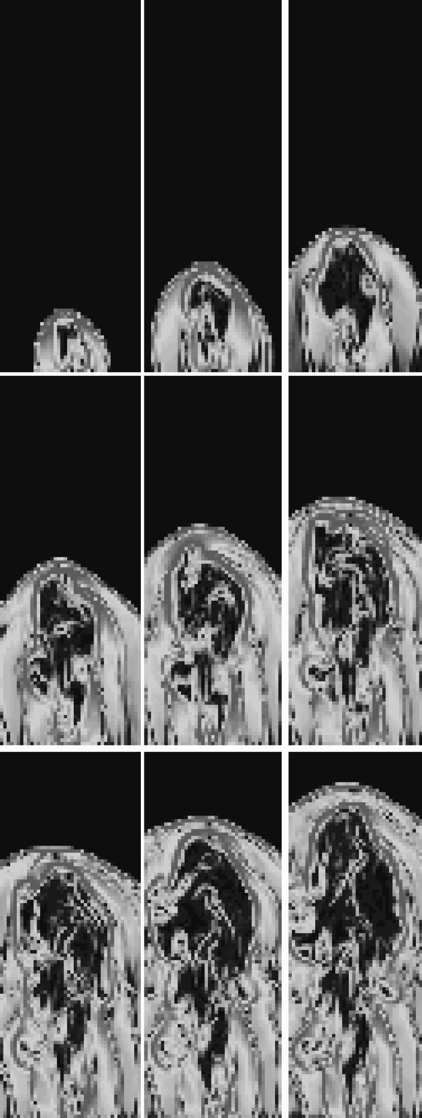
Figure 12: Slices in the plane $x=0$ at equally-spaced intervals during the evolution of the precessed $\gamma=5$ jet. Each panel is a schlieren rendering of the laboratory frame density.

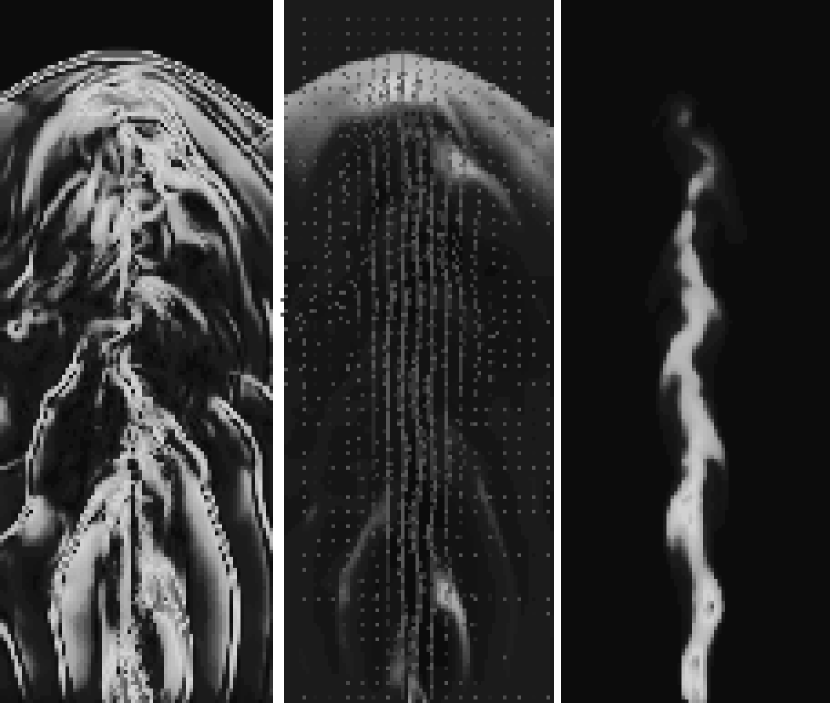
Figure 13: Slices in the plane $x=0$ at the last time step for the precessed $\gamma=5$ jet, showing from left to right: a schlieren render of the pressure, a linear render of the pressure with 3-velocity vectors superposed, and the Lorentz factor; the peak Lorentz factor of $5$ is rendered red, and values of order $1$ are dark blue – the peak values appear as dark regions in a monochrome render. The jet retains its integrity for $\sim 50$ jet-radii, and thereafter rapidly disrupts.

Figure 12 shows a sequence of slices in the plane $x=0$ at equally-spaced intervals during the evolution, using schlieren plots of laboratory frame density. Superficial inspection of the final slice suggests that to a significant extent, the jet has retained its integrity, and is driving a bow not dissimilar to that seen in the unprecessed case. In particular, on average the bow is advancing at $v\sim 0.41$, which is $\sim 63$% the speed with which it advanced in the unprecessed case, suggesting a relatively undiminished jet thrust. However, Figure 13 shows from left to right, a schlieren render of the pressure – there are dramatic variations of pressure along the jet’s path, suggestive of significant dissipation; a linear render of the pressure (dominated by the leading bow) with 3-velocity vectors superposed – evidently the jet’s momentum has been shared with a broad sheath of material; and finally, the Lorentz factor – showing that despite precession, the jet does retain its integrity for almost $50$ jet-radii, but thereafter the flow speed drops dramatically. The asymmetric bow is being driven forward by a flow in which the pressure maintains a high enthalpy, and which is to some extent focussed onto a small area at the bow’s apex.

Figure 14 quantifies this, showing the run of rest frame density, pressure, Lorentz factor and momentum flux (or ‘discharge’), ${\cal F}=\gamma^{2}\left(e+p\right)v_{z}^{2}+p$, along the spine of the flow. This spine was defined by computing weighted, average $x$ and $y$ values in a series of planes $z=$constant, within a cylinder of diameter $6$ jet-radii aligned with the jet inflow (to exclude complex structures near to the edge of the computational domain). Using the Lorentz factor as a weighting function produced a locus barely distinguishable from that found using the momentum flux as a weighting function, leading us to the conclusion that this approach indeed picks out a physically significant core flow. The quantities plotted in Figure 14 are spatial averages within cylindrical pills of one jet radius, aligned locally with the spine. Increasing the radius of these sampling volumes decreased the average Lorentz factor and momentum flux, but did not change the character of the variation of these quantities along the spine. Beyond $50$ jet-radii the Lorentz factor falls well below its initial value and the local flow direction becomes more chaotic.

Indeed, the orientation of the velocity vectors within the jet, relative to the local jet ‘direction’ – defined by the locus of the spine – is a quantity of fundamental importance. Is the flow locally parallel to the jet boundary, with little momentum imparted to the jet’s wall, leading to the expectation that flow disturbances (e.g., shocks) would follow the jet channel, or do fluid elements move more ballistically? The bottom panel of Figure 14 shows the angle between the spine of the flow and the inflow direction (i.e., the $z$-direction) as a dashed line, and the angle between the spine of the flow and the velocity as a solid line. The former changes quite smoothly along the flow, increasing to a value well above that imposed at inflow, in conjunction with a decline in the $z$ component of momentum flux. By $\sim 50$ jet-radii large fluctuations associated with jet disruption become evident. If the velocity vectors tracked the flow, the solid line would remain close to zero. However, until significant disruption of the jet is evident, the angle between the spine of the flow and the velocity closely follows, but lies a little below, the angle of the spine. This is because the velocity vectors are almost entirely along the $z$-axis, with a slight offset (typically $\lesssim 4\arcdeg$) towards the local channel direction (with the potential to change the Doppler boost of emitted radiation by more than $25$%). Thus while there is a weak tendency for velocities to follow the jet channel, the motion is substantially ballistic, with significant momentum imparted to the jet wall, displacing that surface as the flow evolves. Figure 15 shows the evolution of the location of the spine in 9 equally separated planes $z$=constant to a little beyond $50$ jet-radii. (The jet spends too little time further from the inflow to study its evolution there.) The complex pattern of dashed lines that join these points arises because the spine is captured at various phases of precession in the 28 epochs sampled, but the stable, conical path of the spine is evident for tens of jet radii from the inflow.

Interaction between the precessing flow and its cocoon of shocked jet material has imparted a significant ‘forward’ velocity to the latter. Within the broad region delimited by the contact surface between shocked jet and shocked ambient material the entire flow moves forward at a marginally relativistic speed, forming a plateau about a spine of highly relativistic flow. The corresponding velocity distribution for the unprecessed case shows significant forward flowing cocoon material only within a jet’s radius of the jet itself. This contrasts even more dramatically with the results seen in highly underdense jet simulations, e.g., Komissarov and Falle (1996), where the cocoon material shows significant backflow in the laboratory frame (albeit away from the jet, near to the contact surface), with the potential for significant Doppler enfeeblement of its radiation flux. The broad forward flow seen in the current simulation is suggestive of the core-sheath morphology suggested to explain observations implying both relativistic and nonrelativistic motions in the same source, e.g., Hanasz and Sol (1996), and the recent observation of a source with a ‘spine-sheath’ morphology, evident in the polarization map (Attridge et al., 1999). Whether jets that propagate from the sub-parsec scale to the tens of kiloparsec scale can retain their integrity under the influence of large amplitude precession can be answered only through larger scale computations involving a diverging flow, wherein the local scale length to jet radius ratio is bounded.

6 Discussion

We have shown that jets impacting an inclined ambient density gradient are subject to the development of internal waves and oblique shocks. It is impractical to run the simulations to a point where the leading bow shock leaves the computational domain, but we have shown that these internal structures are slow moving, and argued that their driving flows persist long after the bow has passed the deflecting structure; thus an interesting question is the extent to which these internal structures would be observable in maps not dominated by the bow shock (which even if in proximity to the structures of interest, might contribute little to the synchrotron emissivity – e.g., Mioduszewski et al. (1997)). In the simulation with $\gamma=2.5$, $\phi=65\arcdeg$ (see Figure 6) the oblique, high pressure structure upstream of the flow’s head spans the jet in the plane parallel to the ambient density gradient, and in a plane orthogonal to that, constitutes a wedge of extent $\sim 2.75$ jet radii, and maximum width $\sim 0.43$ jet radii. It thus fills $\sim 7$% of the volume of the perturbed jet segment. The peak pressure in this structure is $p_{peak}\sim 0.38$, while in the adjacent cocoon $p_{ext}\sim 0.2$, and in the initial state $p_{int}=0.05$. If the emission is optically thin, with spectrum $\propto\nu^{-\alpha}$, there is equipartition between radiating particles and random magnetic field ($u_{e}\sim u_{B}$), and the number of radiating particles is proportional to the internal energy and thus the pressure, the emissivity is $j\propto p^{\left(\alpha+3\right)/2}$ (Mioduszewski et al., 1997). For $\alpha=0.5$ the emissivity of the oblique structure is $\sim 35$ times that of the quiescent jet. Allowing for the $\sim 7$% filling factor, this structure would be $\sim 2.4$ times brighter than a corresponding segment of unperturbed jet. The simulation with $\gamma=5$ and $\phi=35\arcdeg$ (see Figure 11) also shows a prominent oblique internal structure in the final time frame; again, the structure spans the jet in a plane parallel to the ambient gradient and its section orthogonal to this direction approximates an ellipse with major axis tilted slightly with respect to the jet’s inflow direction. The filling factor is $\sim 50$%. The corresponding pressure values are $p_{peak}\sim 0.78$, $p_{ext}\sim 0.2$ and $p_{int}=0.27$ (the initial pressure being higher than in the slow jet case for fixed Mach number). Following the same arguments as used above to estimate the component flux, it follows that this structure would be $\sim 3.2$ times brighter than a corresponding segment of unperturbed jet. We conclude that where jets are disturbed by ambient density structure, jet emission may be enhanced by a significant factor ($2-3$) locally, with little impact on the jet’s global dynamics.

A simple prescription for the appearance of the precessed jet (see Figure 12) cannot be readily given, as the structure is highly asymmetric, and while the local jet boundary evolves at subrelativistic speed, significant Doppler boosting is associated with the instantaneous flow velocity, and varies with observer location, even for observers with the same inclination to the inflow axis. Maps are being computed by C. M. Swift, following the approach described by Mioduszewski et al. (1997) and these results will be presented elsewhere. For the purpose of characterizing brightness variations that might be associated with such flows, here we consider the variation of a simple estimator of the source intensity along the flow’s spine. We have computed an effective emissivity ${\cal E}=p^{\left(\alpha+3\right)/2}{\cal D}^{2}$ as a function of distance along the spine, where ${\cal D}=1/\gamma\left(1-\beta\cos\theta\right)$, the Doppler factor, and the boost is appropriate for stationary, bounded flows (Cawthorne, 1991). The well-defined, high Lorentz factor channel evident in Figure 13 illustrates that at least within a jet radius of the spine, the internal flow conditions are quite uniform, and that the significantly Doppler boosted flow suffers little divergence before disruption just upstream of the bow. The observed intensity will be determined by integrating the emissivity across the Doppler boosted flow for some line of sight, and given the cross-flow uniformity, and comparable line of sight depth for each flow segment, ${\cal E}$ provides a reasonable estimator of the source brightness. We have adopted $\alpha=0.5$, and an angle of view with respect to the inflow axis $\theta^{\prime}=10\arcdeg$, the latter being of interest as the critical cone of the inflowing jet (with $\gamma=5.0$) is $\sin^{-1}\left(1/\gamma\right)\sim 11.5\arcdeg$. The detailed run of ${\cal E}$ along the spine depends upon the azimuthal angle chosen. However, for all cases, a narrow peak in Doppler factor occurs between $10$ and $20$ jet radii along the spine, and convolved with the broad pressure peak at that location (see Figure 14) always leads to a substantial intensity enhancement: the peak ‘intensity’ is typically $6$ to $10$ times that in the ‘intensity’ minimum immediately downstream. Beyond $20$ jet radii, significant (by a factor of $2$ or more) fluctuations in ‘intensity’ occur, the details of which depend on observer orientation, but which are not uniquely tied to variations in the underlying pressure distribution or Doppler factor – although there is a trend for pressure fluctuations to underpin the ‘intensity’ variations as the head is approached.

The flow thus exhibits a core-jet morphology, in which individual features can move both towards and away from the jet’s origin – according to the phase of precession – by a number of jet radii. In particular, if the core is associated with the inner-most region where emissivity and high Doppler boost conspire to produce a high intensity component, the location of that component will not be stable to within a few jet-radii. As the precession time scale is likely to be long compared with the time scale for propagation of an individual component along the flow, this will have minimal effect on a sequence of VLBI measurements that define the trajectory of one component. However, it could lead to long-term changes in the relative position of stationary components, and change the inner jet orientation so as to influence the details of the interaction of propagating and stationary components, e.g., as seen in $4C~{}39.25$ (Alberdi et al., 2000). This precessed flow has a number of characteristics exhibited by BL Lac objects: a core-jet morphology, with stationary, or slowly moving components, and a flow that appears to dissipate rather close to the core. Jets associated with QSOs may typically be followed further than those associated with BL Lac objects, so perhaps one facet of the class distinction relates to the amplitude of precessional perturbation to which the jet is subjected. Evidently a small helical perturbation (transverse velocity of order 1% of longitudinal velocity) does not lead to disruption of the flow (Hardee et al., 2001). Our immediate goal is to generate a well-sampled grid of simulations for a range of Lorentz factor and precession cone semi-angle, to establish both the largest amplitude of precession for which flows of a given Lorentz factor avoid macroscopic break-up, and the physical origin of that break up. The extent to which propagating shocked fluid, thought to explain moving VLBI components, will follow the helical channel, or follow approximately ballistic trajectories, is also a subject for future study.

Figure 1: The relativistic shock tube. The left column shows the entire computational domain and the right panels show blow ups of the region encompassing the shock. The solid line is the numerical solution for a shock propagating along $x$, and the dashed line is the analytic solution from Thompson (1986). The computation was taken to a time of 0.626 on a grid of 1365 cells. The top panel shows the rest density ($n$), the middle panel the pressure ($p$), and the bottom panel the Lorentz factor ($\gamma$).

Figure 3: Cuts showing the laboratory frame density ($R$) and Lorentz factor ($\gamma$) for the final time slice of the blastwave problem for cuts along the coordinate directions and lines that bisect these directions.

Figure 5: Rest frame density, pressure and Lorentz factor as a function of distance along the jet axis ($Z$), at $0.2$, $0.4$, $0.6$ and $0.8$ jet-radii, for the 2D simulation (solid lines), and a 3D simulation (dashed lines) of the same resolution. Insets in the density and pressure panels show the respective variable upstream of the flow’s head. Density and pressure variations upstream of the Mach disk are of higher amplitude in the 2D case, with peaks at smaller $Z$ for cuts further from the jet axis, while the 3D case shows a more widely distributed, but lower amplitude series of variations.

Figure 14: From top to bottom: the run of rest frame density ($n$), pressure ($p$), Lorentz factor ($\gamma$) and momentum flux ($\cal F$) along the spine of the precessed flow. The bottom panel shows the local angle between the spine and the inflow direction (dashed line) and the local angle between the velocity vector and the spine (solid line). The plot in the lowest panel is terminated where the flow direction becomes ill-defined.

Figure 15: The evolution of the spine of the precessed jet, at 9 locations $z=$constant labeled in jet-radii. Each mark shows the location of the spine at one of 28 time slices, and the sense of evolution is given by the joining dashed lines.

References

- Alberdi et al. (1999) Alberdi, A., Gómez, J. L., Marcaide, J. M., Marscher, A. P., & Pérez-Torres, M. A. 1999, in BL Lac Phenomenon, ed. L. O. Takalo & A. Sillanpää (San Francisco: ASP), 452
- Alberdi et al. (2000) Alberdi, A., Gómez, J. L., Marcaide, J. M., Marscher, A. P., & Pérez-Torres, M. A. 2000, A&A, 361, 529
- Aller et al. (1999) Aller, H. D., Hughes, P. A., Freedman, I., & Aller, M. F. 1999,in BL Lac Phenomenon, ed. L. O. Takalo & A. Sillanpä(̈San Francisco: ASP), 45
- Aloy et al. (1999) Aloy, M. A., Ibáñez, J. M., Martí, J. M., Gómez, J.-L., & Müller, E. 1999, ApJ, 523, L125
- Attridge et al. (1999) Attridge, J. M., Roberts, D. H., & Wardle, J. F. C. 1999, ApJ, 518, L87
- Berger (1982) Berger, M. 1982, Dissertation, Stanford University
- Berger and Colella (1989) Berger, M., & Colella, P. 1989, J. Comp. Phys., 82, 67
- Bicknell and Begelman (1996) Bicknell, G. V., & Begelman, M. C., 1996, ApJ, 467, 597
- Blandford and McKee (1976) Blandford, R. D. & McKee, C. F. 1976, Phys. Fluids, 19, 1130
- Bowman (1994) Bowman, M. 1994, MNRAS, 269, 137
- Cawthorne (1991) Cawthorne, T. V. 1991, in Beams and Jets in Astrophysics, ed. P. A. Hughes (Cambridge: Cambridge Univ. Press), 187
- Daly and Marscher (1988) Daly, R. A., & Marscher, A. P. 1988, ApJ, 334, 539
- Dar (1998) Dar, A. 1998, ApJ, 500, L93
- Denn, Mutel and Marscher (1999) Denn, G. R., Mutel, R. L., & Marscher, A. P. 1999, ApJS, 129, 61
- Duncan and Hughes (1994) Duncan, G. C., & Hughes, P. A. 1994, ApJ, 436, L119
- Einfeldt (1988) Einfeldt, B. 1988, SIAM J. Numerical Analysis, 25, 294
- Godunov (1959) Godunov, S. K. 1959, Mat. Sb., 47, 271
- Hanasz and Sol (1996) Hanasz, M., & Sol, H. 1996, A&A, 315, 355
- Hardee and Clarke (1992) Hardee, P. E., & Clarke, D. A. 1992, ApJ, 400, L9
- Hardee et al. (2001) Hardee, P. E., Hughes, P. A., Rosen, A., & Gomez, E. A. 2001, ApJ, 555, 744
- Hardee et al. (1998) Hardee, P. E., Rosen, A., Hughes, P. A., & Duncan, G. C. 1998, ApJ, 500, 599
- Harten et al. (1983) Harten, A., Lax, P., & Van Leer, B. 1983, SIAM Rev., 25, 35
- Heinz and Begelman (1997) Heinz, S., & Begelman, M. C. 1997, ApJ, 490, 653
- Higgins et al. (1999) Higgins, S. W., O’Brien, T. J., & Dunlop, J. S. 1999, MNRAS, 309, 273
- Hjellming and Rupen (1995) Hjellming, R. M., & Rupen, M. P. 1995, Nature, 375, 464
- Hughes et al. (1989a) Hughes, P. A., Aller, H. D., & Aller, M. F. 1989a, ApJ, 341, 54
- Hughes et al. (1989b) Hughes, P. A., Aller, H. D., & Aller, M. F. 1989b, ApJ, 341, 68
- Icke (1991) Icke, V. 1991, in Beams and Jets in Astrophysics, ed. P. A. Hughes (Cambridge: Cambridge Univ. Press), 232
- Jorstad et al. (2001) Jorstad, S. G., et al. 2001, ApJS, 134, 181
- Koide et al. (1996) Koide, S., Sakai, J.-I., Nichikawa, K.-I., & Mutel, R. L. 1996, ApJ, 464, 724
- Komissarov and Falle (1996) Komissarov, S. S., & Falle, S. A. E. G. 1996, in Energy Transport in Radio Galaxies and Quasars, ed. P. E. Hardee, A. H. Bridle, & J. A. Zensus (San Francisco: ASP ), 173
- Komissarov and Falle (1998) Komissarov, S. S., & Falle, S. A. E. G. 1998, MNRAS, 297, 1087
- Leahy (1991) Leahy, P. J. 1991, in Beams and Jets in Astrophysics, ed. P. A. Hughes (Cambridge: Cambridge Univ. Press), 100
- Lister et al. (1998) Lister, M. L., Marscher, A. P., & Gear, W. K. 1998, ApJ, 504, 702
- Lobanov and Zensus (1996) Lobanov, A. P., & Zensus, J. A. 1996, in Energy Transport in Radio Galaxies and Quasars, ed. P. E. Hardee, A. H. Bridle, & J. A. Zensus (San Francisco: ASP ), 109
- Marscher and Gear (1985) Marscher, A. P. & Gear, W. K. 1985, ApJ, 298, 114
- Marscher et al. (1997) Marscher, A. P. et al. 1997, BAAS, 190, 5106
- Martí, et al. (1994) Martí, J. M., Müller, E., & Ibáñez, J. M. 1994, A&A, 281, L9
- Martí, et al. (1995) Martí, J. M., Müller, E., Font, J. A., & Ibáñez, J. M. 1995, ApJ, 448, L105
- Martí, et al. (1997) Martí, J. M., Müller, E., Font, J. A., Ibáñez, J. M. Z., & Marquina, A. 1997, ApJ, 479, 151
- Mendoza and Longair (2001a) Mendoza, S., & Longair, M. S. 2001, MNRAS, 324, 149
- Mendoza and Longair (2001b) Mendoza, S., & Longair, M. S. 2001, astro-ph/0109125
- Mioduszewski et al. (1997) Mioduszewski, A. J., Hughes, P. A., & Duncan, G. C. 1997, ApJ, 476, 649
- Mirabel and Rodríguez (1994) Mirabel, I. F., & Rodríguez, L. F. 1994, Nature, 371, 46
- Mirabel and Rodríguez (1995) Mirabel, I. F., & Rodríguez, L. F. 1995, Annals of the New York Academy of Sciences, eds. H. Böhringer, G. E. Morfil, & J. Trümper, 759, 21
- Mutel et al. (1990) Mutel, R. L., Phillips, R. B., Su, B., & Bucciferro, R. R. 1990, ApJ, 352, 81
- Muxlow and Garrington (1991) Muxlow, T. W. B., & Garrington, S. T. 1991, in Beams and Jets in Astrophysics, ed. P. A. Hughes (Cambridge: Cambridge Univ. Press), 52
- Myers (1978) Myers, P. C. 1978, ApJ, 225, 380
- Nichikawa et al. (1997) Nichikawa, K.-I., et al. 1997, ApJ, 483, L45
- Nichikawa et al. (1998) Nichikawa, K.-I., et al. 1998, ApJ, 498, 166
- Perlman et al. (1999) Perlman, E. S., Biretta, J. A., Zhou, F., Sparks, W. B., & Macchetto, F. D. 1999, AJ, 117, 2185
- Polatidis and Wilkinson (1998) Polatidis, A. G., & Wilkinson, P. N. 1998, MNRAS, 294, 327
- Rosen et al. (1999) Rosen, A., Hughes, P. A., Duncan, G. C., & Hardee, P. E. 1999, ApJ, 516, 729
- Shaffer et al. (1987) Shaffer, D. B., Marscher, A. P., Marcaide, J., & Romney, J. D. 1987, ApJ, 314, L1
- Thompson (1986) Thompson, K. 1986, J. Fluid Mech., 171, 365
- Tingay et al. (1995) Tingay, S. J., et al. 1995, Nature, 374, 141
- Valtonen and Lehto (1997) Valtonen, M. J., & Lehto, H. J. 1997, ApJ, 481, L5
- van Putten (1993) van Putten, M. H. P. M. 1993, ApJ, 408, L21
- van Putten (1994) van Putten, M. H. P. M. 1994, Int. J. Bif. & Chaos, 4, 57
- van Putten (1996) van Putten, M. H. P. M. 1996, ApJ, 467, L57
- Wardle et al. (1994) Wardle, J. F. C., Cawthorne, T. V., Roberts, D. H., & Brown, L. F. 1994, ApJ, 437, 122
- Wen et al. (1997) Wen, L., Panaitescu, A., & Laguna, P. 1997, ApJ, 486, 919
- Wilson (1987) Wilson, M. J. 1987, MNRAS, 226, 447
- Zensus (1997) Zensus, J. A. 1997, ARA&A, 35, 607