On the recent history of star formation in the BCD galaxy VII Zw403.

Abstract

Here we attempt to infer the recent history of star formation in the BCD galaxy VII Zw403, based on an analysis that accounts for the dynamics of the remnant generated either by an instantaneous burst or by a continuous star formation event. The models are restricted by the size of the diffuse X-ray emitting region, the H_α luminosity from the star-forming region and the superbubble diffuse X-ray luminosity.

We have re-observed VII Zw403 with a better sensitivity corresponding to the threshold H_α flux $8.15\times 10^{-17}$ erg cm^-2 s^-1. The total H_α luminosity derived from our data is much larger than reported before, and presents a variety of ionized filaments and incomplete shells superimposed on the diffuse H_α emission. This result has a profound impact on the predicted properties of the starburst blown superbubble. Numerical calculations based on the HST H_α data, predict two different scenarios of star formation able to match simultaneously all observed parameters. These are an instantaneous burst of star formation with a total mass of $5\times 10^{5}$ M_⊙ and a star-forming event with a constant SFR = $4\times 10^{-3}$ M_⊙ yr^-1, which lasts for 35 Myrs. The numerical calculations based on the energy input rate derived from our observations predict a short episode of star formation lasting less than 10 Myrs with a total star cluster mass $\sim(1-3)\times 10^{6}$ M_⊙. However, the five main star-forming knots are sufficiently distant to form a coherent shell in a short time scale, and still keep their energies blocked within local, spatially separated bubbles. The X-ray luminosities of these is here shown to be consistent with the ROSAT PSPC diffuse X-ray emission.

1 Introduction

It has recently been recognized that the star formation activity in galaxies is very irregular in time, and many examples of major burst episodes exhibit an extremely high star formation rate concentrated in well localized space regions (Terlevich 1996). It is also now well known that starbursts (SBs) cause an emission that dominates the entire host galaxy luminosity and their mechanical energy input rate is expected to cause major structural changes in the surrounding interstellar medium (ISM). In this respect it has become of great interest to study the properties of the resultant large-scale expanding superbubbles which, powered by the violently injected newly processed matter, establish the time scale for mixing with the ISM (Tenorio-Tagle 1996, Silich et al. 2001). In extreme cases, the superbubbles are thought to break out of the galactic discs leading to an effective mass and energy transport into the low density halos or even into the intergalactic medium via a superwind (Heckman et al. 1990).

Starbursts in the local universe are also assumed to be good representatives of the star-forming activity at high redshifts. This concept defines their cosmological interest as key laboratories for studying the ISM, the transport of supernovae processed metals, as well as the chemical evolution of galaxies and of the intergalactic medium. The resulting structure in the ISM due to mechanical energy injected by SBs is very similar to the interstellar wind-blown bubbles around single massive stars (see Weaver et al. 1977 for their four zone model), although the much larger energy input rate in SBs leads rapidly to much larger scales. Hydrodynamical simulations (see Tenorio-Tagle & Bodenheimer 1988, Bisnovatyi-Kogan & Silich 1995 and references therein; Suchkov et al. 1994; Silich & Tenorio-Tagle 1998; D’Ercole & Brighenti 1999; Strickland & Stevens 2000) currently include differential galactic rotation, radiative cooling, strong density gradients between the disk and the halo and thus are able to follow the moment of breakout, as well as the fragmentation of the expanding outer shell via Rayleigh - Taylor instabilities and the venting of the superbubble hot interior gas, either into the intergalactic space, or into the host galaxy halo (the blowout phenomenon).

Most of the up to-date simulations have been performed under the assumption of a constant energy deposition rate, as expected from an instantaneous burst model. However, studies of the stellar population in OB associations related to young ($\tau_{OB}<10$ Myr) Large Magellanic Cloud (LMC) bubbles (see Oey & Smedley, 1998 and references therein) have demonstrated that “realistic” energy input rates are very different from the assumed constant energy input rates used in numerical simulations. Thus the instantaneous burst assumptions may not be applicable to all cases. Here we attempt to establish a method of comparison between the theory of superbubbles and the observations of remnants produced by massive star formation in galaxies. Two possible modes of star formation, instantaneous and extended bursts, are taken into consideration. For both cases the mechanical luminosity, ultraviolet photon output, mass returned to the ISM, and the fraction of each in metals, all as a function of time, are estimated. On the other hand we have the observed parameters: the H_α or H_β luminosity which can be directly related to the SFR under the assumption that all photons are used up in the ionized region. One can also estimate the size and luminosity of the X-ray remnant. In some cases the remnants may have slowed down sufficiently to display their outer expanding shells, either in the optical or in HI observations, or both, giving further information about the size, expansion speed, and mass behind the outer shock. A comparison with the theory also requires some preconception of the galaxy’s ISM, which can as a first approximation be derived from HI observations and the inferred dynamical mass. However, one also needs to make an assumption about the fraction of this gas locked up in dense clouds and immersed into a less dense ISM background.

With the aim of establishing a method to confront theory with observations that may lead us to infer the recent star formation history of galaxies, the blue compact dwarf (BCD) VII Zw403 is thoroughly analyzed. Section 2 derives the main properties of coeval and extended star formation modes. Section 3 summarizes the main observational properties of our target. Section 4 presents a summary of the hydrodynamical calculations aimed at matching the observed properties. The results of the calculations and our main findings are discussed in Section 5.

2 Star formation

Following the observational evidence in support of the concept of a continuous star formation spread over 10 - 20 Myr or more (Herbst & Miller 1982, Stahler 1985, Coziol et al. 2001), Shull & Saken (1995) have discussed five possible tracks of the star formation rate (SFR) time evolution, including both the time span of star formation, and possible time variations in the initial mass function (IMF). Here we examine one of their cases: a constant SFR spread over a finite time interval $\tau_{SB}$. We compare its intrinsic properties with the standard instantaneous model. The simple model discussed below can be generalized to more sophisticated cases with a time dependent SFR and a variable IMF.

2.1 The properties of starbursts

Let us assume an instantaneous burst characterized by an IMF with an exponent $\alpha$,

$$f(m)=\frac{(\alpha-2)M_{SB}}{M_{low}^{2-\alpha}-M_{up}^{2-\alpha}}m^{-\alpha},$$ (1)

where $M_{SB}$ is the total mass of the SB cluster, and $M_{low}$ and $M_{up}$ are the lower and upper cut-off masses, respectively. From this one can calculate the expected energy and mass input rates.

2.1.1 The mechanical energy input rate.

The mechanical energy deposition from a starburst should include both the energy injection via stellar winds and from supernova explosions. Here the early mechanical energy injection (before the first supernova explosion at $t$ = $t_{sn}$) has been approximated by a constant value $L_{w}$, which adds the contribution of all individual massive stars in the cluster. This value can easily be scaled from the template of Leitherer & Heckman, 1995 (hereafter LH95) for a starburst with a total mass of 10⁶ M_⊙ within the mass range $M_{low}$ = 1 M_⊙ and $M_{up}$ = 100 M_⊙

$$L_{SB}=L_{LH}\frac{M_{SB}}{M_{LH}}=Const,\qquad t\leq t_{sn},$$ (2)

where $M_{SB}$ is the total stellar mass considered, $M_{LH}$ = 10⁶ M_⊙ and $L_{LH}$, following LH95 was set equal to $10^{39}$ erg s^-1.

After a time ($t>t_{sn}$) the energy released via supernova explosions dominates the SB mechanical energy deposition, and then the energy released by the SB as a function of time is defined by the expression

$$E_{SB}(t)=\int_{M(t)}^{M_{up}}E_{SN}f(m){\rm d}m=$$

$$\frac{(\alpha-2)}{(\alpha-1)}\frac{M_{SB}E_{SN}}{M_{low}^{2-\alpha}-M_{up}^{2-\alpha}}\left(M^{1-\alpha}(t)-M_{up}^{1-\alpha}\right),$$ (3)

where $M(t)$ is the mass of the stars exploding as supernovae after an evolutionary time $t$. For simplicity, the energy released per supernova ($E_{SN}$) is assumed to be independent of the progenitor mass and equal to 10⁵¹ erg.

The energy input rate from the SB at the supernova dominated stage is then

$$L_{SB}=\frac{{\rm d}E_{SB}(t)}{{\rm d}t}=$$

$$-\frac{(\alpha-2)M_{SB}E_{SN}M^{-\alpha}(t)}{M_{low}^{2-\alpha}-M_{up}^{2-\alpha}}\frac{{\rm d}M}{{\rm d}t},\quad t>t_{sn}.$$ (4)

The lifetime of the massive stars can be inferred from the approximations of Chiosi et al. (1978) and Stothers (1972). Then the function $M(t)$ has the form:

$$\frac{M(t)}{10M_{\odot}}=\left\{\begin{array}[]{lcl}(9\times 10^{6}/t)^{2};\hfill\ 30M_{\odot}\leq M\leq 100M_{\odot}\\[5.69046pt] (3\times 10^{7}/t)^{5/8};\hfill\ 7M_{\odot}\leq M\leq 30M_{\odot}.\end{array}\right.$$ (5)

Substituting the time derivative of $M(t)$ into equation (2.1.1) one obtains

$$L_{SB}=\left\{\begin{array}[]{lcl}\frac{2(\alpha-2)M_{SB}E_{SN}}{M_{low}^{2-\alpha}-M_{up}^{2-\alpha}}\frac{M^{1-\alpha}(t)}{t},\hskip 2.84544ptt_{sn}\leq t\leq t_{30}\\[5.69046pt] \frac{5}{8}\frac{(\alpha-2)M_{SB}E_{SN}}{M_{low}^{2-\alpha}-M_{up}^{2-\alpha}}\frac{M^{1-\alpha}(t)}{t},\hskip 2.84544ptt_{30}\leq t\leq t_{7}\end{array}\right.$$ (6)

where $t_{30}$ and $t_{7}$ are the stellar lifetimes for a 30 M _⊙ and a 7 M _⊙ star, respectively.

2.1.2 Mass deposition

Before the first supernova explosion, the mass injected by a star cluster results from individual stellar winds calculated as

$$M_{ej}(t)=\int_{0}^{t}2L_{SB}/V_{w}^{2}dt,\quad t\leq t_{sn},$$ (7)

where the collective wind terminal velocity is assumed to be $V_{w}=2000$ km s^-1. Afterwards, the mass injection is dominated by supernovae and one can neglect the contribution from stellar winds. During the supernova dominated stage, the total ejected mass as a function of time may be approximated by (see Silich et al. 2001):

$$M_{ej}(t)=M_{SB}\frac{M(t)^{2-\alpha}-M_{up}^{2-\alpha}}{M_{low}^{2-\alpha}-M_{up}^{2-\alpha}},\quad t>t_{sn}.$$ (8)

Following Silich et al. (2001) we assume that the gas ejected by supernovae includes all the newly synthesized metals, and thus the mass in ejected metals as a function of time is

$$M_{metals}=$$

$$\frac{(\alpha-2)M_{SB}}{M_{low}^{2-\alpha}-M_{up}^{2-\alpha}}\int_{M(t)}^{M_{up}}Y_{metals}(m)m^{-\alpha}{\rm d}m,$$ (9)

where $Y_{metals}$ is a particular element yield. One can then use, for example, oxygen as tracer of the metalicity caused in the interior of superbubbles. In such a case the oxygen yield can be approximated by analytical fits to the stellar evolutionary tracks of Maeder (1992) and Woosley et al. (1993), which account for the mass loss due to stellar winds (see Silich et al. 2001). The mean metalicity inside a superbubble is then defined by the ratio of the wind and supernovae ejected oxygen to the total mass within the superbubble $M_{in}=M_{ej}+M_{ev}$, which includes also the mass thermally evaporated from a cold outer shell ($M_{ev}$):

$$Z_{O}=\frac{M_{ej}(O)/Z_{\odot}(O)+Z_{ISM}M_{ev}}{M_{in}},$$ (10)

where $Z_{ISM}$ and $Z_{O}$ are both in the solar units, $Z_{\odot}(O)=0.0083$ (Grevesse et al. 1996).

2.1.3 The $UV$ output

For a coeval star cluster, the $UV$ photon production rate remains almost constant until the most massive star in the cluster begins to move away from the main sequence, soon becoming a supernova. From this moment onward, the $UV$ flux rapidly decays (Beltrametti et al. 1982). We approximate this evolutionary track by the power function

$$N_{UV}=\left\{\begin{array}[]{lcl}N^{0}\frac{M_{SB}}{M_{LH}},\qquad\qquad\quad 0\leq t\leq t_{sn}\\[5.69046pt] N^{0}\frac{M_{SB}}{M_{LH}}(t_{sn}/t)^{5},\qquad t>t_{sn}.\end{array}\right.$$ (11)

The initial flux ($N^{0}$) was normalized to the 10⁶ M_⊙ standard model of LH95, and was taken to be 9 $\times 10^{52}$ photons s^-1. If all $UV$ photons are trapped within a star forming region, then the H_α expected luminosity $L_{H_{\alpha}}$ follows from a simple transformation (LH95): $L_{H_{\alpha}}=1.36\times 10^{-12}N_{UV}$ erg s^-1.

2.2 Continuous star formation

If the star formation process is not coeval but is instead spread over a time $\tau_{SB}$, one can approximate it by a series of $N_{tot}$ instantaneous sequential mini bursts separated by a $\Delta\tau=\tau_{SB}/N_{tot}$. One can further assume that all mini bursts would have the same mass $M_{i}=M_{SB}/N_{tot}$ and IMFs and would evolve independently according to their own clocks set upon formation:

$$t_{i}=t-(i-1)\Delta\tau,$$ (12)

where $t$ is an evolutionary time, and $i$ is the mini burst number. Then the number of mini bursts at any given time $t$ is

$$n(t)=\left\{\begin{array}[]{lcl}Int(t/\Delta\tau)+1,\quad if\quad t\leq\tau_{SB}\\[5.69046pt] N_{tot},\quad if\quad t>\tau_{SB}.\end{array}\right.$$ (13)

The cumulative intrinsic properties (mechanical energy input rate, mass injection and the number of $UV$ photons or the H_α luminosity) can be found by simply adding the mini burst parameters:

$$L_{SB}=\sum_{i=1}^{i=n(t)}L_{i},$$ (14)

$$M_{ej}=\sum_{i=1}^{i=n(t)}M_{ej,i},$$ (15)

$$N_{UV}=\sum_{i=1}^{i=n(t)}N_{UV,i}.$$ (16)

Note that the input from each mini burst should be set to zero whenever their individual evolutionary time $t_{i}$ exceeds the lifetime of the less massive star which can explode as supernova; that is once $t_{i}$ becomes larger than their intrinsic $t_{7}$.

The global energy properties of star formation events derived from this simple model are in a good agreement with the two extreme cases (instantaneous and continuous star formation) of LH95 and are presented in Figure 1. For comparison a value of $\alpha$ = 2.35 has been assumed as well as a stellar range of masses between 1 M_⊙ and 100 M_⊙.

Figure 1a compares the mechanical energy input rates derived for a 10⁶ M_⊙ stellar cluster formed during a $\tau_{SB}$ = 1 Myr (hereafter the instantaneous burst), 20 Myr and 50 Myr. The solid line shows the rapid rise in the coeval case, which reaches a maximum immediately after the onset of supernova explosions, and then drops to values $\sim$ 10^40.2 erg s^-1 to remain almost constant up to the end of the supernova activity ($\sim$ 50 Myr). For the $\tau_{SB}$ = 20 Myr event, the maximum energy deposition is delayed in time, and converges with the 1 Myr values after approximately 25 Myr. The energy deposition rate for $\tau$ = 50 Myr star forming episode suffers an even longer delay, to reach values similar to the maximum input from the previous two models, and then slowly decays without reaching a uniform value throughout the 100 Myr of its evolution.

The production rate of $UV$ photons (see Figure 1b) is highly dependent on the star formation time considered. For the 1 Myr starburst the $UV$ flux reaches its maximum value ($\sim$ 9 $\times 10^{52}$) at t = $\tau_{SB}$, and remains constant during the first 4 Myr. It then falls very steeply, reaching before 10 Myr of evolution, values more than two orders of magnitude smaller than its maximum value. The 20 Myr and 50 Myr clusters acquire their uniform constant value after 4 Myr of evolution, and then upon completion of their star formation phase, their $UV$ photon output also rapidly decays with time.

The rate at which mass is ejected by the massive star cluster is shown in Figure 1c. The total ejected mass ($\sim 40\%$ of the star cluster mass) and the total oxygen mass released by supernovae (about 2$\%$ of the total mass turned into stars) is clearly the same at the end of the evolution in the three cases considered. There are however substantial delays for the larger the value of $\tau_{SB}$.

3 The main observational properties of VII Zw403

VII Zw403 is a BCD galaxy considered in recent years in many discussions related to star formation histories and possible impact of dwarf systems on the surrounding intergalactic medium. Although Tully et al. (1981) proposed that the galaxy might be a member of M81 group, more recent distance determinations (Lynds et al. 1998) locate it about 1.5 Mpc further away at 4.5 Mpc distance. Therefore it can be considered an isolated galaxy (Schulte-Ladbeck et al., 1999).

The X-ray observations (Papaderos et al. 1994; Fourniol 1997) added more interest to the system, as they revealed an extended kpc-scale region of diffuse X-ray emission. These observations account for approximately 85% of the total X-ray luminosity (L${}_{X,total}\approx 2.3\times 10^{38}$ erg s^-1) from the central unresolved core, while the remaining 15% is spread over the central kpc-scale region. The high-resolution data reported by Lira et al. (2000) revealed a strong point X-ray source displaced to the west with respect to the main H_α emission. This is most probably a powerful (L${}_{X}\sim 10^{38}$ erg s^-1) binary system. However, the kpc-scale diffuse component was not confirmed by these observations, possibly due to the low sensitivity of the HRI.

The total dynamical mass of the galaxy is $2\times 10^{8}$  $\hbox{M}_{\odot}$, with approximately 20% or $4\times 10^{7}$  $\hbox{M}_{\odot}$  constituting the neutral hydrogen phase (Thuan & Martin, 1981). VII Zw403 does not exhibit a regular rotation, but rather turbulent random motions of individual neutral hydrogen clumps with $\Delta V_{t}\approx 30$ km s^-1 (Thuan & Martin, 1981). This value is taken as the velocity dispersion which supports the ISM against the self gravity of the galaxy. The extension of the neutral hydrogen halo R_ISM is not well known, but if the average ratio of the HI size to the optical size is accepted to be f = 2.4 (Thuan & Martin, 1981), the HI halo radius R_HI is about 1.9 kpc. A similar result is obtained if one assumes that the galaxy boundary occurs at the location where the escape velocity drops below the ISM random velocity $\Delta V_{t}$.

Lynds et al. (1998) showed that the stellar population of VII Zw403 contains not only young blue main-sequence stars, but also a much older evolved population that can be traced up to 1-2 Gyrs back in time. They also studied the five centrally concentrated associations of young stars, with ages smaller than 10 Myr, and that in H_α emission appear to be surrounded by local small shells with radii $\sim 100$ pc. Schulte-Ladbeck et al. (1999) provided a near infrared single star photometry of the galaxy and confirmed that compact, young star-forming regions are embedded into a much older, low surface brightness halo.

3.1 New observations

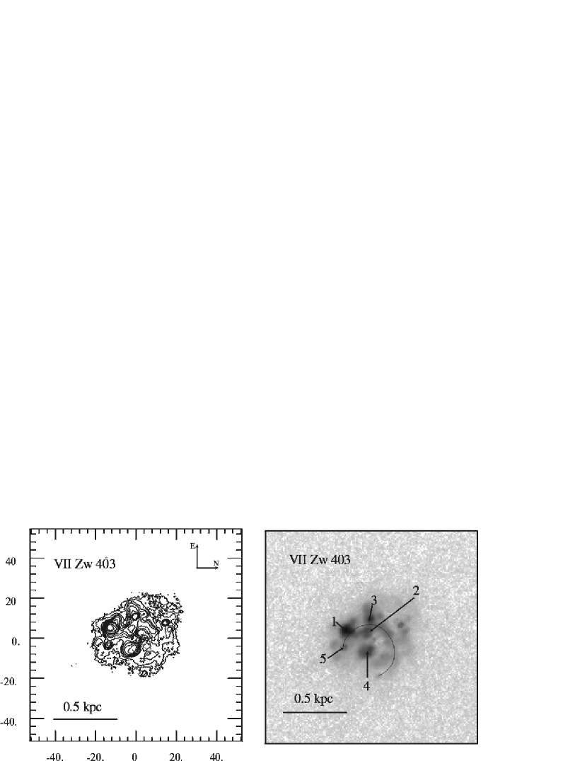
Figure 2: The narrow-band H_α image of VII Zw403. The left panel shows isocontours map of the continuum substracted H_α image. The right panel presents grey scale map of H_α emission in logarithmic scale. The lowest H_α isocontour level corresponds to the threshold value $8.15\times 10^{-17}$ erg s^-1 cm^-2. Isocontours are equispaced in logaritmic scale.

We present here new narrow-band images of VII Zw403 centered on the $H_{\alpha}$ line and on the adjacent continuum (Figure 2) which were taken in August 1997 at the 2.2-m telescope of the German–Spanish Astronomical Observatory at Calar Alto (Almería, Spain). The instrumentation consisted of the Calar Alto Faint Object Spectrograph (CAFOS) and a $2048\times 2048$ SiTe CCD chip, with a pixel size of 0.53 arcsec, and an un-vignetted circular field of view of about 11 arcmin in diameter (14.4 kpc at the accepted distance to the galaxy of 4.5 Mpc). The averaged seeing was 1.5 arcsec.

The image reduction was conducted using standard procedures available in IRAF. Each image was corrected for bias using an average bias frame, and was flattened by dividing by a mean twilight flat field image. After, they were registered (for each filter we took a set of dithered exposures) and combined to obtain the final frame, with cosmic rays removed and bad pixels cleaned. The average sky level was estimated by computing the mean value within various boxes surrounding the object, and subtracted out as a constant. Flux calibration was done through the observation of spectrophotometric stars from Oke (1990). For more details about data reduction and calibration refer to Cairós et al. (2001). We calculated the integrated H_α flux out to the limiting isophote with a level equal to $2.5\times rms$ of the background. In our case this threshold is $8.15\times 10^{-17}$ erg s^-1 cm^-2. The H_α flux was corrected for Galactic extinction following Burstein & Heiles (1984). No correction for internal extinction was performed.

Our H_α image shown in Figure 2 displays a variety of shapes and structures which deserve discussion. Besides the starburts knots, labeled 1 - 5 after Lynds et al. (1998), we detect a much fainter and extended well structured diffuse emission. The largest obvious feature is a broken to the SW shell-like structure, 250 pc in radius, which we associate with knot 4. Knot 2 is almost overlapping in projection along its Eastern rim.

On top of features and structures which appear to build a network of connecting knots, there is down to our limiting flux a diffuse-smooth emission which engulfs them all and most certainly results from photons leaking out of the main emitting knots.

The total H_α luminosity is higher than reported previously. Clearly our limiting flux is much lower than that of Lynds et al. (their Figure 2). Our data recovers the low intensity H_α emission and thus provides a more precise estimate of the total H_α luminosity.

The spatial resolution of the HST image (Lynds et al. , 1998) also allows for the detection of a much smaller H_α mini-bubble (cocoon), associated with knot 1. This bubble has similar energy to that inferred for the large superbubble reported above, however it seems much less evolved. The energy dumped by the cluster energizing knot 1 has not been able to sweep and displace so efficiently the surrounding ISM out of which it formed.

The above result has a profound impact on the modeling of starbursts. Clearly during the first few Myr of evolution every center of star formation disperses its high density parental cloud. It is only after this task has been completed that the various star forming centers that compose a starburst would be able to jointly build up a large-scale superbubble.

The main observational properties of VII Zw403 from the above mentioned literature and our own observations are summarized in the Table 1.

4 A numerical model for VII Zw403

A successful model has to be able to match simultaneously all observed parameters. In the case of VII Zw403 these are: the size ($R_{sh}\sim$ 1 kpc) of the diffuse X-ray emitting region, the H$\alpha$ and the X-ray (L${}_{x}\sim 3\times 10^{37}$ erg s^-1) luminosities. Note that Lynds et al. (1998) give a total value L${}_{H\alpha}\sim 1.8\times 10^{39}$ erg s^-1 which is smaller than the total flux detected by our observations (L${}_{H_{\alpha}}\sim 4.7\times 10^{40}$ erg s^-1). We have used both of these values in our search of a successful model of VII Zw403. Note also that the values derived from X-ray observations are doubtful and require confirmation (Bomans, 2001). VII Zw403 presents various nuclear centers of star formation, each of which have managed to locally structure the ISM, and thus present a number of loops or broken shells with radii $\sim 100$ pc. Another important fact is that available observations display neither an HI nor an HII or X-ray large-scale shell surrounding the diffuse X-ray emission. This fact can be ascribed to a remnant evolving along its quasi-adiabatic phase, or to a neutral hydrogen shell brightness that falls below the detection limit.

All considered models assume that the observed HI mass occupies a smooth low density disc-halo distribution, although an important fraction of it ($20\%<f_{c}<95\%$) is in a dense cloud component. This has a major impact on the evolution of remnants as it affects both the time required to reach a given size, as well as the resultant X-ray luminosity produced within the superbubble. Our models also assume that the ISM is supported in hydrostatic equilibrium in the galaxy gravitational field by the turbulent gas pressure produced by the random gas motions with an effective velocity dispersion $\Delta V_{t}$ (see Tomisaka & Bregman, 1993; Silich & Tenorio-Tagle, 1998). An example of the resultant initial ISM smooth component density distribution is shown in Figure 3.

The calculations were carried out with our 3D Lagrangian code, which accounts for the enrichment of the hot superbubble interior by the metals ejected via supernova explosions (Silich et al. 2001). Using oxygen as tracer, we derived the time dependent superbubble interior gas metalicity, which was then used in our calculations of the diffuse X-ray emission. As there are no firm observational restrictions on the VII Zw403 star formation timescale, we have examined different scenarios of the recent star formation activity in this galaxy. Two sets of models have been considered: an instantaneous burst, and an extended star formation episode. We have associated an instantaneous burst with the 1 Myr event and calculated the SB parameters following the prescriptions of section 2. In all coeval models considered, the energy input rate has been derived from the assumed mass of the star forming cluster. In the extended star formation scenarios we used instead the observed H_α luminosity to derived the star formation rate from our continuous star formation model (see section 2). This SFR was then transformed into a total star cluster mass and energy input rate, for the various assumed values of $\tau_{SB}$, as it was considered in section 2. A Salpeter initial mass function, with upper and lower cutoff masses 1 and 100 M_⊙ respectively, was assumed for all models.

We then calculated the time $\tau_{dyn}$ that superbubbles need to reach the observed 1 kpc diffuse X-ray radius. A value of $\tau_{dyn}$ implies an age from which one can calculate the central H_α luminosity and the integrated superbubble diffuse X-ray emission for every model. The results of the calculations for instantaneous burst models are summarized in Table 2. The various models are labeled with two separate indices that represent the logarithm of the SB mass (also indicated in column 2) and the fraction of the ISM assumed to be in the smooth component respectively. The preceding letter “I” indicates that all of these are instantaneous burst models. Four different star cluster masses have been considered: $10^{5}$, $5\times 10^{5}$, $10^{6}$ and $10^{7}$ $\hbox{M}_{\odot}$. Column 3 indicates the fraction of the ISM mass assumed to be stored in clouds. The calculated dynamical time $\tau_{dyn}$ is presented in column 4. After this time the shock wave has expanded to 1kpc radius, and the relevant parameters from the model can be compared with the observed values. The calculated number of $UV$ photons, the H_α luminosity (under assumption that all $UV$ photons are trapped within a SB region), and the resultant superbubble diffuse X-ray luminosity, are presented in columns 5, 6 and 7 respectively. Column 8 indicates whether the superbubbles evolve along a quasi-adiabatic track (A), or have made a transition to a radiative phase (R) before reaching the 1 kpc radius. The two possible modes of expansion imply different properties for the swept-up matter: either material is still too hot to radiate effectively and thus occupies the outer 20% of the remnant volume, or it has collapsed into a thin and cold outer shell, while being exposed to the ionizing radiation.

The second set of models assumes an extended phase of star formation. The results of the calculations for these models are summarized in Table 3. The various models are labeled again with two separate indices that now represent the star formation time $\tau_{SB}$ (in Myr) and the fraction of the ISM in the smooth component. The letter “C” indicates the continuous star forming mode, for which episodes lasting 5, 10, 20 and 40 Myr have been assumed. In all these models we assumed the same SFR ($4\times 10^{-3}$  $\hbox{M}_{\odot}$  yr^-1). Column 2 indicates the total stellar mass, and columns 3 to 8 list the same variables considered in Table 2. In all of these models we assumed that the photons currently produced by the stellar clusters are all used up in reestablishing the ionization of the central HII region. This fact is supported by the large HI mass present in VII Zw403.

The resulting H_α luminosity, and the time dependent mechanical energy input rate, are shown in Figures 4a and b respectively.

5 Discussion

Table 2 shows that both low (10⁵ $\hbox{M}_{\odot}$) and high ($10^{7}$ $\hbox{M}_{\odot}$) mass SB models are completely inconsistent with the VII Zw403 parameters derived from Lynds et al. (1998) data. Indeed, the low mass models lead to a very slow expansion speed, which makes them reach the 1kpc size only after 10 Myr, even in the lowest density case with a cloud mass filling factor f_c = 90% of the observed HI mass. After this time the most massive stars have left the main sequence and exploded as supernovae, causing a fast drop in the number of emitted $UV$ photons and consequently in the H_α luminosity of the associated HII region. This luminosity in all low SB mass cases is several orders of magnitude below the currently observed value. The high mass models on the other hand, are too energetic, produce an exceedingly high X-ray emission, and an overwhelming $UV$ photons flux when the superbubble radius reaches 1kpc.

The intermediate mass SBs ($5\times 10^{5}-10^{6}\thinspace\hbox{$\hbox{M}_{\odot}$}$) are in better agreement with observations. However, for the emitted number of $UV$ photons to be consistent with the value derived from the observed H_α luminosity, the smooth component of the ISM has to contain only a small ($\sim 5\%$) fraction of the observed HI mass. The shock wave blown by coherent SN explosions into this low density medium remains adiabatic when it reaches a 1 kpc radius (see Table 2). Therefore, in these models (I5.7_5, I6.0_5) an essential fraction of the X-ray emission ($\sim 80\%$ in the model I5.7_5 and $\sim 50\%$ in the model I6.0_5) arises from the outer adiabatic shell of swept-up matter that should occupy the outer $\leq 20\%$ of the remnant volume. However, this is not resolved in the available X-ray maps.

From the results in Table 3, it is clear that for a reasonable agreement between the observed parameters of VII Zw403 and a continuous star formation scenario, the episode of star formation should last no less than the dynamical time required for the superbubble to reach the 1 kpc radius.

The best continuous star-forming model (C40_70), with a SFR = $4\times 10^{-3}$  $\hbox{M}_{\odot}$  yr^-1, $\tau_{SB}=40$ Myr, and 30% of the total ISM mass in the dense cloud component, requires about 35 Myr for the outer shock to reach a radius $\sim$ 1 kpc. In this model an extended gaseous halo cannot completely prevent gas loss from the galaxy and allows a final shell speed slightly in excess of the escape velocity. The H_α luminosity is not an issue in this case as it is exactly the amount used to derive the constant SFR. The time evolution of the superbubble diffuse X-ray emission is shown in Figure 5 for different ISM models. Initially the X-ray luminosity grows rapidly with time, following the energy input rate and mean hot gas metalicity time evolution. It reaches a maximum value after 10 - 20 Myrs, and then remains almost constant up to the end of the star forming activity. The maximum X-ray luminosity is larger in models with a larger smooth ISM component, and matches the value observed in VII Zw403 when the smooth component of the ISM amounts to 70% of the observed HI mass. Note that we stopped our calculations when the shock fronts reached the assumed galactic ISM cut-off position (1.9 kpc). This causes the breaks in the X-ray curves around 30 Myr and 50 Myr, for the f${}_{c}=0.9$ and f${}_{c}=0.6$ models respectively.

Note that for these moderate ISM densities and the relevant mechanical luminosities (see Figure 4b), the shell of swept-up matter becomes radiative after a short time $\tau_{cool}\approx 2.3\times 10^{4}n_{ISM}^{-0.71}L_{38}^{0.29}$ yr (Mac Low & McCray, 1988). However, this is not detected in the available HI maps. One can then claim that the large-scale shell is photo-ionized by radiation escaping the central HII region, and thus it should be most easily observed in H_α light. However, note that if $\sim 80\%$ of the $UV$ photon flux is being used to ionize gas around the central star clusters, as it is assumed to be for the totality of clusters 1 and 2 in VII Zw403 (Lynds et al., 1998), then the rest of the photons (N${}_{esc}=0.25L_{H\alpha}/1.36\times 10^{-12}$ s${}^{-1}\approx 3.25\times 10^{50}$ s^-1) would be free to ionize the outer ISM. If the number of $UV$ photons trapped within the neutral smooth component is negligible, they will ionize the neutral outer shell. Such a shell would appear as a 1 kpc diffuse H_α emitting feature with brightness

$$B=\frac{1.36\times 10^{-12}N_{esc}}{64\pi R_{sh}^{2}}\theta^{2}\approx 10^{-17}\,erg\,s^{-1}\,cm^{-2},$$ (17)

where $\theta=1.5$ arcsec is the averaged seeing. However, this is below our detection limit ($8.15\times 10^{-17}erg\,s^{-1}\,cm^{-2}$), and thus the H_α emission excess expected at the bubble outer shell is unlikely to be detected. Approximately an order of magnitude better sensitivity has to be reached to confirm this possible model.

So far it appears that the remnants caused by the two completely different recent star-forming histories considered here are able to explain the observables in VII Zw403. In all of our models however, we have also calculated the time dependent mixing of the metals freshly ejected by supernovae with the matter thermally evaporated from the outer shell. Figure 6 shows the time evolution of the mean inner gas metalicity (using oxygen as a tracer, see Silich et al. 2001) predicted for the superbubbles in the two extreme cases able to match the observations of VII Zw403. Both cases show a superbubble interior metalicity largely different to that of the ISM detected in the optical regime (Z${}_{ISM}=0.06Z_{\odot}$, see Table 1). Enormous differences are found in the coeval case which rapidly acquires several times Z_⊙. On the other hand, the continuous star formation, although presenting high metalicity values, never surpasses Z_⊙. This result could be used as a discriminator able to discard various possible recent histories of star formation in VII Zw403. However, as it is likely that the swept-up matter in the shell preserves the same metalicity as the unperturbed ISM (see Tenorio-Tagle, 1996), it will be difficult to distinguish between the metalicities of two overlaid X-ray components in the instantaneous burst case.

A close comparison of the HST observations and our data however has led us to realize that, although $UV$ photons may escape their production centers and HII regions causing the extended diffuse ionized gas, the mechanical energy from the various star-forming centers has not had sufficient time to drive a large-scale remnant. This has not happened, despite the 5 - 10 Myr of evolution of the various subgroups in the galactic nucleus. It seems that the five star-forming centers are sufficiently distant from each other, that their mechanical energy is still currently being used to build up individual local shells. The largest H_α shell around star cluster 4 with a radius $\sim$ 250 pc is not yet enclosing, and not even in contact with the HII regions and smaller shells produced by the other star forming centers present in the galaxy.

This structure thus invalidates the assumption often made, that a given mechanical luminosity derived from the H_α luminosity of a galaxy can be directly used in theoretical models as acting upon a smooth medium from the start of the calculation.

VII Zw403 is clearly indicating that there may be an important leakage of $UV$ photons out from the centers of star formation, causing an extended diffuse ionized region around a starburst. However, for the mechanical energy of the various well separated centers of star formation to start working together in the production of a large-scale remnant, a longer time scale is required. A sufficient period needs to allow for the multiple shock waves to merge and overlap with each other, clearly implying a longer time the larger the separation between subgroups and the denser the ISM may be around the various star-forming centers.

This time scale is particularly relevant when one tries to match the remnants produced by the stellar activity in a badly (spatially) resolved or distant galaxy, for which one can nevertheless derive a good estimate of its H_α luminosity. If for example one will ignore the detailed structure of the ionized gas in the VII Zw403 and use the mechanical energy input rate derived directly from the total H_α luminosity, then little difference will be found between the coeval and the continuous star formation models. To fit simultaneously the larger H_α luminosity ($4.7\times 10^{40}$ erg s^-1) and the X-ray luminosity derived from the PSPC data, both models would require very similar star cluster masses $(1-3)\times 10^{6}$ M_⊙, a similar ISM structure with a large cloud mass filling factor ($\sim 95\%$), and a similar superbubble dynamical age (5 - 8 Myr). In both cases the expanding shell would remain adiabatic when the remnant reaches the 1 kpc radius. That is, if one takes the total H_α luminosity to derive the mechanical energy input rate and the bubble time evolution without knowing the ionized gas spatial distribution, one would predict a very powerful and young remnant. The delay caused by depositing the derived total mechanical luminosity locally into the different knots, clearly changes the outcome. Nevertheless, the high level of energy deposition (L${}_{SB}\approx 2\times 10^{40}$ erg s^-1) predicts (see Silich & Tenorio-Tagle, 2001) that the ISM of VII Zw403 will be blown away after a few tens of Myrs.

This leads to another possible interpretation of the observed X-ray emission, that is coming from the local bubbles generated by the various stellar subgroups. Take for example the OB associations 1 and 4 for which we know the total stellar mass, the ionizing flux, the age, and the local bubble radius. From these we have derived both analytic (Chu & Mac Low, 1990), and numerical (Silich et al., 2001) estimates of the present bubble X-ray luminosity. Note that local bubble kinematic ages estimated from the H_α radii and expansion velocities ($\sim 1$ Myr) are much smaller than the stellar cluster ages derived from the massive star isochrones, which are 4 - 6 Myrs (Lynds et al. 1998). This discrepancy is often observed in the LMC bubbles (Oey & Smedley, 1998), and most probably is related to the recent bubble blowout from the host molecular cloud (Silich & Franco, 1999). We have assumed a mean stellar cluster age (5 Myrs) as a better indicator of the bubble time evolution. One can then estimate the X-ray emission from the local bubbles if the energy input rate and the surrounding gas density n_c are known:

$$L_{x}=10^{36}ZI(\tau)L_{38}^{33/35}n_{c}^{17/35}t_{7}^{19/35},$$ (18)

where Z is the hot X-ray emitting gas metalicity, I$(\tau)$ is a dimensionless integral whose value is close to unity, the energy input rate L₃₈, and the evolutionary time t₇, measured in $10^{38}$ erg s^-1 and $10^{7}$ yr units respectively. We derive the appropriate star cluster mass, and its mechanical luminosity from our SB model, and use them to estimate the surrounding gas density from the standard (Weaver et al. 1977) bubble model:

$$n_{c}=\left(\frac{267pc}{R_{sh}}\right)^{5}L_{38}t_{7}^{3},$$ (19)

These results were compared (see table 4) with the numerical calculations assuming a time-dependent mechanical energy input rate and time-dependent hot gas metalicity. Note that the inferred X-ray luminosities show a good agreement with the observations. The large differences between the numerical and analytical estimations of the surrounding gas density results from the different mechanical energy input rates (a constant value for analytical models and increasing with time rate for numerical calculations).

6 Conclusion

Here we have discussed the recent history of star formation and a possible nature of the diffuse X-ray emission in the nearby BCD galaxy VII Zw403. Two possible scenarios of star formation have been considered: an instantaneous burst, and an extended episode of star formation.

To construct the numerical model we have provided new narrow-band observations of VII Zw403 centered on the H_α line with a long exposure time corresponding to the threshold H_α flux $8.15\times 10^{-17}$ erg cm^-2 s^-1. These observations reveal a variety of ionized filaments and incomplete shells superimposed on the diffuse H_α emission that most certainly result from the photons leaking out of the main star-forming centers. The largest feature is the 250 pc broken shell associated with stellar association 4. The total H_α luminosity derived from our observations, L${}_{H_{\alpha}}=4.7\times 10^{40}$ erg s^-1, is much larger than reported before. This has a profound impact on the predicted properties of the starburst blown superbubble.

The numerical models based on the HST H_α data require either an instantaneous burst of star formation with a total mass of $5\times 10^{5}$ M_⊙, or a star formation episode with a constant SFR = $4\times 10^{-3}$ M_⊙ yr^-1 lasting 35 Myr. The models however require radically different structures of the galactic ISM and imply very different properties of the resulting remnant.

The best coeval model assumes most of the ISM to be locked up within high density clouds, and only $\sim 5\%$ of the observed neutral hydrogen mass is in the smooth component. The hydrodynamical calculations also predict the outer shell to be adiabatic after reaching a 1 kpc radius, and to contribute 50 - 80% of the observed diffuse X-ray emission. The bubble evolutionary time is estimated to be $\tau_{dyn}\approx 7$ Myr when its expansion speed is $\approx 200$ km s^-1.

The best continuous star formation model requires of much higher density in the smooth ISM component, with only $\sim 30\%$ of the HI mass concentrated in dense clouds. This leads to a much smaller bubble expansion velocity (V${}_{exp}\approx 35$ km s^-1), larger evolutionary time ($\tau_{dyn}\sim 35$ Myr), and a rapid cooling within the outer shell. That is, this model predicts a low brightness HI shell surrounding the diffuse 1 kpc X-ray region. This shell may also show up in ${H\alpha}$ if exposed to the $UV$ flux from the central cluster. The inner gas metalicities are also predicted to be very different in these two cases.

The numerical calculations based on the high energy input rate derived from our observations require an instantaneous burst or a short episode of star formation with SFR $\sim 0.1$ M_⊙ yr^-1 lasting less than 10 Myr with similar total stellar cluster masses $(1-3)\times 10^{6}$ M_⊙ and most of the ISM ($\sim 95\%$) locked up within high density clouds. The comparison of the energy input rate derived from our ${H\alpha}$ data with the theoretical limits, implies that the entire ISM and metals produced by the current episode of star formation are going to be ejected from the galaxy after the coherent superbubble is formed.

It appears that the five main star-forming knots are sufficiently distant to form a coherent shell in a short time scale, while keeping their energies blocked within local, spatially separated bubbles. This provides a time delay that must be considered when developing a numerical model for the coherent superbubble driven by a number of young stellar clusters. Numerical calculations show that the X-ray luminosities from young local bubbles are in a good agreement with the ROSAT PSPC data. This agreement indicates that the observed diffuse component of the X-ray emission may be related to the small centrally concentrated bubbles, rather than to the coherent 1 kpc structure. Further observations with the XMM-NEWTON observatory is expected to be able to recover the real nature of the diffuse X-ray emission and the recent history of star formation in this galaxy.

We thank D. Bomans for his comments and suggestions regarding the X-ray data. We also thank the anonymous referee for his detailed report that greatly improved our paper. Finally we also thank Edward Chapin for his careful reading of the manuscript.

This work has been supported by the Spanish grants PB97-1107 and AYA2001-3939, and the Mexico (CONACYT) project 36132-E.

Table 1: VII Zw403 observational properties

Parameter		Reference	Comments
Distance	4.5 Mpc	1
The galaxy total mass	$2\times 10^{8}$ M⊙	2
The galaxy ISM mass	($4-7)\times 10^{7}$ M⊙	1, 2	from HI observations
The radius of the HI halo	$\sim 1.9$ kpc		not well known, see text
The ISM gas velocity
dispersion	$\sim$ 30 km s-1	2
The ISM gas metalicity	(0.05 - 0.06)Z⊙	3
The total Hα flux	$(195\pm 4)\times 10^{-13}$ ergs cm-2 s-1	our data	integrated out to
			the limiting isophote
The total Hα luminosity	$1.8\times 10^{39}$ ergs s-1	1
	$4.7\times 10^{40}$ ergs s-1	our data
Hα shell radii
- Large	$\sim 250$ pc	our data	around association 4
- Small	$\sim 80$ pc	1	around association 1
Diffuse X-ray emission:	$(1.9-2.3)\times 10^{38}$ ergs s-1	4, 5	ROSAT PSPC data
- Unresolved core	$\sim 85\%$		not confirmed by
- Extended diffuse emission	$\sim 15\%$		ROSAT HRI data
X-ray flux from the point
source	$9\times 10^{-13}$ ergs cm-2 s-1	6	ROSAT HRI data

References: 1) Lynds et al., 1998 2) Thuan & Martin, 1981 3) Schulte-Ladbeck et al., 1999 4) Papaderos et al., 1994 5) Fourniol, 1997 6) Lira et al., 2000

Table 2: A 1 kpc bubble parameters for instantaneous burst models

Model	MSB	fc	$\tau_{dyn}$	$N_{UV}$	LHα	Lx	Shell state
	$\hbox{M}_{\odot}$	%	Myr	photons s-1	erg s-1	erg s-1
1	2	3	4	5	6	7	8
I5.0_10	105	90	12.5	7.4$\times 10^{48}$	1.0 $\times 10^{37}$	1.2 $\times 10^{37}$	R
I5.0_40	105	60	21.8	4.3$\times 10^{47}$	5.8 $\times 10^{35}$	2.2 $\times 10^{37}$	R
I5.0_70	105	30	29.7	8.7$\times 10^{46}$	1.2 $\times 10^{35}$	2.8 $\times 10^{37}$	R
I5.7_5	$5\times 10^{5}$	95	6.7	9.5$\times 10^{50}$	1.3 $\times 10^{39}$	4.2 $\times 10^{37}$	A
I5.7_10	$5\times 10^{5}$	90	7.9	4.3$\times 10^{50}$	5.8 $\times 10^{38}$	1.6 $\times 10^{38}$	A
I5.7_40	$5\times 10^{5}$	60	12.0	4.5$\times 10^{49}$	6.1 $\times 10^{37}$	1.8 $\times 10^{38}$	R
I5.7_70	$5\times 10^{5}$	30	15.5	1.3$\times 10^{49}$	1.7 $\times 10^{37}$	2.3 $\times 10^{38}$	R
I6.0_5	106	95	6.0	3.5$\times 10^{51}$	4.8 $\times 10^{39}$	3.5 $\times 10^{37}$	A
I6.0_10	106	90	6.8	2.0$\times 10^{51}$	2.7 $\times 10^{39}$	1.5 $\times 10^{38}$	A
I6.0_40	106	60	9.8	2.7$\times 10^{50}$	3.7 $\times 10^{38}$	4.5 $\times 10^{38}$	R
I6.0_70	106	30	12.0	9.1$\times 10^{49}$	1.1 $\times 10^{38}$	5.5$\times 10^{38}$	R
I7.0_10	107	90	4.7	1.5$\times 10^{53}$	2.0 $\times 10^{41}$	3.3$\times 10^{38}$	A
I7.0_40	107	60	5.8	4.4$\times 10^{52}$	5.9 $\times 10^{40}$	1.7$\times 10^{39}$	A
I7.0_70	107	30	6.3	3.0$\times 10^{52}$	4.1 $\times 10^{40}$	8.1$\times 10^{39}$	A

Table 3: A 1 kpc bubble parameters for continuous star formation models

Model	MSB	fc	$\tau_{dyn}$	$N_{UV}$	LHα	Lx	Shell state
	$\hbox{M}_{\odot}$	%	Myr	photons s-1	erg s-1	erg s-1
1	2	3	4	5	6	7	8
C5_10	2.1$\times 10^{4}$	90	22.3	1.3$\times 10^{47}$	1.6$\times 10^{35}$	1.3$\times 10^{36}$	R
C5_40	2.1$\times 10^{4}$	60	50.5	1.5$\times 10^{45}$	2.1$\times 10^{33}$	1.1$\times 10^{36}$	R
C10_10	4.1$\times 10^{4}$	90	20.0	1.5$\times 10^{48}$	2.0$\times 10^{36}$	3.6$\times 10^{36}$	R
C10_40	4.1$\times 10^{4}$	60	34.5	4.0$\times 10^{46}$	5.4$\times 10^{34}$	6.6$\times 10^{36}$	R
C10_70	4.1$\times 10^{4}$	30	59.0	1.7$\times 10^{45}$	2.3$\times 10^{33}$	no	R
C20_10	8.2$\times 10^{4}$	90	19.5	1.3$\times 10^{51}$	1.8$\times 10^{39}$	5.8$\times 10^{36}$	R
C20_40	8.2$\times 10^{4}$	60	29.4	1.7$\times 10^{48}$	2.3$\times 10^{36}$	1.6$\times 10^{37}$	R
C20_70	8.2$\times 10^{4}$	30	37.5	1.6$\times 10^{47}$	2.2$\times 10^{35}$	4.3$\times 10^{37}$	R
C40_10	1.6$\times 10^{5}$	90	19.5	1.3$\times 10^{51}$	1.8$\times 10^{39}$	6.3$\times 10^{36}$	R
C40_40	1.6$\times 10^{5}$	60	29.0	1.3$\times 10^{51}$	1.8$\times 10^{39}$	1.9$\times 10^{37}$	R
C40_70	1.6$\times 10^{5}$	30	35.1	1.3$\times 10^{51}$	1.8$\times 10^{39}$	3.2$\times 10^{37}$	R

Table 4: Parameters from individual bubbles

	Association 1	Association 4
$UV$ flux	$5\times 10^{50}$ s-1	$7\times 10^{50}$ s-1
Star cluster age	5 Myr	5 Myr
Star cluster mass	$4.7\times 10^{4}$ M⊙	$6.6\times 10^{4}$ M⊙
Shell radius	79 pc	250 pc
	Analytic model	Analytic model
ISM number density	$1.1\times 10^{3}$ cm-3	4.9 cm-3
Bubble X-ray luminosity	$3.5\times 10^{38}$ Z I($\tau$) erg s-1	$3.4\times 10^{37}$ Z I($\tau$) erg s-1
	Numerical model	Numerical model
ISM number density	40 cm-3	0.2 cm-3
Bubble X-ray luminosity	$1.8\times 10^{38}$ erg s-1	$2.1\times 10^{37}$ erg s-1
Hot gas mean metalicity	$Z_{O}=1.8Z_{\odot}$	$Z_{O}=0.6Z_{\odot}$

Figure 1: The intrinsic properties of instantaneous and extended starbursts. The panels present: the energy input rates (a), the ionizing photon flux (b), and the total mass, and the fraction of this in oxygen, ejected by instantaneous and extended bursts of star formation (c), all as a function of time. In all the panels solid lines represent the instantaneous ($\tau_{SB}$ = 1 Myr) burst, dotted lines indicate the results for the $\tau_{SB}$ = 20 Myr and dashed lines those for $\tau_{SB}$ = 50 Myr.

Figure 3: The gas density distribution for models assuming 90% of the ISM mass to be stored in clouds.

Figure 4: Inferred parameters for VII Zw403. From the observed H_α luminosity one can infer the SFR and thus the ionizing photon flux. If all these quantities remain constant for a $\tau_{SB}$ as shown in panel (a) for the central region H_α luminosity, one can then infer the run of the mechanical energy input rate (b).

Figure 5: Comparison of the X-ray luminosity (diffuse component) for models with $\tau_{SB}$ = 40 Myr and different fractions of the interstellar gas in the cloudy component (M_cl).

Figure 6: The metalicity of the superbubble as a function of time for two best models related with the HST data. Oxygen is used as a tracer, arrows indicate metalicities at the time superbubbles reach the 1 kpc radius.

References

- (1) Bisnovatyi-Kogan, G. S. & Silich, S. A.: 1995, Rev. Mod. Phys. 67, 661
- (2) Beltrametti, M., Tenorio-Tagle, G. & Yorke, H. W. 1982, A&A, 112, 1
- (3) Bomans, D. 2001, Rev. Mod. Astroph., 14, 297
- (4) Burstein, D. & Heiles, C. 1984, ApJS, 54, 33
- (5) Cairós, L. M., Caon, N., Vílchez, J. M., González-Pérez, N. & Muñoz-Tuñón, C., 2001, ApJ., in press
- (6) Chiosi, C., Nasi, E. & Sreenivasan, S. P. 1978, A&A, 63, 103
- (7) Chu, Y.-H.& Mac Low, M.-M., 1990, ApJ, 365, 510
- (8) Coziol, R., Doyon, R. & Demers, S. 2001, MNRAS, 325, 1081
- (9) D’Ercole, A. & Brighenti, F. 1999, Mon. Not. Roy. Ast. Soc., 309, 941
- (10) Fourniol, N. 1997, Thesis ’X-ray and optical observations of the HII galaxies’.
- (11) Grevesse, N., Noels, A. & Sauval, A. J. 1996, ASP Conf. Ser., eds. Holt, S. S. & Sonnebom, G. 99, 117
- (12) Heckman, T. M., Armus, L. & Miley, G. K. 1990, ApJS, 74, 833
- (13) Herbst, W. & Miller, D. P. 1982, AJ, 87, 1478
- (14) Leitherer, C. & Heckman, T. M. 1995, ApJS, 96, 9
- (15) Lira P., Lawrence A. & Johnson, R. A. 2000, MNRAS, 319, 17
- (16) Lynds, R., Tolstoy, E., O’Neil, E. J. Jr. & Hunter D. A. 1998, AJ, 116, 146
- (17) Maeder, A. 1992, A&A, 264, 105
- (18) Mac Low, M.-M. & McCray, R. 1988, ApJ, 324, 776
- (19) Oey, M. S. & Smedley, S. A. 1998, AJ, 116, 1263
- (20) Oke, J. B. 1990, AJ, 99, 1621
- (21) Papaderos, P., Fricke, K. J., Thuan, T. X. & Loose, H.-H. A&A, 1994, 116, L13
- (22) Schulte-Ladbeck, R. E., Hopp, U., Greggio, L. & Crone M. M. 1999, AJ, 118, 2705
- (23) Shull, J. M. & Saken, J. M. 1995, ApJ, 444, 663
- (24) Silich, S. & Tenorio-Tagle, G. 1998, MNRAS, 299, 249
- (25) Silich, S. & Franco, J. 1999, ApJ, 522, 863
- (26) Silich, S., Tenorio-Tagle, G. Terlevich, R., Terlevich, E. & Netzer, H. 2001, MNRAS, 324, 191
- (27) Silich, S. & Tenorio-Tagle, G. 2001, ApJ, 552, 91
- (28) Stahler, S. W. 1985, ApJ, 293, 207
- (29) Stothers, R. 1972, ApJ, 175, 431
- (30) Strickland D. K. & Stevens I. R. 2000, MNRAS, 314, 511
- (31) Suchkov, A., Balsara, D., Heckman, T. & Leitherer, C. 1994, ApJ. 430, 511
- (32) Tenorio-Tagle, G. 1996, AJ, 111, 1641
- (33) Terlevich, R. 1996, in 11th IAP Astrophysical Meeting, The Interplay Between Massive Star Formation, the ISM and Galaxy Evolution, ed. D. Kunth, B. Guiderdoni, M. Heydari-Malayeri, & T.X. Thuan (Institut d’Astrophysique, Paris), 3
- (34) Thuan, X. T. & Martin, G. E. 1981, ApJ, 247, 823
- (35) Tomisaka, K. & Bregman, J. N. 1993, PASJ, 45, 513
- (36) Tully, R. B., Boesgaard, A. M., Dyck, H. M. & Sckempp, W. V. 1987, ApJ, 246, 38
- (37) Weaver R., McCray R., Castor J., Shapiro P. & Moore R. 1977, ApJ, 218, 377
- (38) Woosley, S. E., Langer, N. & Weaver, T. A. 1993, ApJ, 411, 823