Triaxial stellar systems following the ${\bf r^{1/n}}$ luminosity law: an analytical mass–density expression, gravitational torques and the bulge/disc interplay

Abstract

We have investigated the structural and dynamical properties of triaxial stellar systems whose surface brightness profiles follow the $r^{1/n}$ luminosity law – extending the analysis of Ciotti (1991) who explored the properties of spherical $r^{1/n}$ systems. A new analytical expression that accurately reproduces the spatial (i.e. deprojected) luminosity density profiles (error less than 0.1%) is presented for detailed modelling of the Sérsic family of luminosity profiles. We evaluate both the symmetric and the non–axisymmetric components of the gravitational potential and force and compute the torques as a function of position. For a given triaxiality, stellar systems with smaller values of $n$ have a greater non–axisymmetric gravitational field component. We also explore the strength of the non–axisymmetric forces produced by bulges with differing $n$ and triaxiality on systems having a range of bulge–to–disc ratios. The increasing disc–to–bulge ratio with increasing galaxy type (decreasing $n$) is found to heavily reduce the amplitude of the non–axisymmetric terms, and therefore reduce the possibility that triaxial bulges in late–type systems may be the mechanism or perturbation for non–symmetric structures in the disc.

Using seeing–convolved $r^{1/n}$–bulge plus exponential–disc fits to the K–band data from a sample of 80 nearby disc galaxies, we probe the relations between galaxy type, Sérsic index $n$ and the bulge–to–disc luminosity ratio. These relations are shown to be primarily a consequence of the relation between $n$ and the total bulge luminosity. In the K–band, the trend of decreasing bulge–to–disc luminosity ratio along the spiral Hubble sequence is predominantly, although not entirely, a consequence of the change in the total bulge luminosity; the trend between the total disc luminosity and Hubble type is much weaker.

1 Introduction

As the quality of photometric data has improved over the years (largely due to the use of CCDs), the applicability of a fitting-function which can account for variations in the curvature of a light profile has been demonstrated for elliptical galaxies (Capaccioli 1987, 1989; Davies et al. 1988; Caon, Capacciolli & D’Onofrio 1993; Young & Currie 1994; Graham et al. 1996), and for the bulges of spiral galaxies (Andredakis, Peletier & Balcells 1995; Seigar & James 1998; Moriondo, Giovanardi & Hunt 1998; Khosroshahi, Wadadekar & Kembhavi 2000; Prieto et al. 2001; Graham 2001; Möllenhoff & Heidt 2001). These systems are not universally described with either an exponential profile or an $r^{1/4}$ law (de Vaucouleurs 1948, 1959), but rather a continuous range of light profile shapes exist which are well described by the Sérsic (1968) $r^{1/n}$ model.

In ellipticals, the shape parameter $n$ from the Sérsic model is strongly correlated with the other global properties derived independently of the $r^{1/n}$ model, such as: total luminosity and effective radius (Caon et al. 1993; Young & Currie 1994, 1995; Jerjen & Bingelli 1997; Trujillo, Graham & Caon 2001), central velocity dispersion (Graham, Trujillo & Caon 2001) and also central supermassive black hole mass (Graham et al. 2001). Additionaly, the spiral Hubble type has been shown to correlate with the bulge index $n$ such that early–type Spiral galaxy bulges have larger values of $n$ than late–type spiral galaxy bulges (Andredakis et al. 1995; Graham 2001). This correlation arises from the fact that the index $n$ is well correlated with the bulge–to–disc luminosity ratio (B/D; see, e.g. Simien & de Vaucouleurs 1986) and this is one of the parameters used to establish morphological type (Sandage 1961).

Given the abundance of observational work and papers now using the Sérsic model, it seems timely that a theoretical study is performed on realistic, analytical models following the $r^{1/n}$ law. Structural and dynamical properties of isotropic, spherical galaxies following $r^{1/n}$ models have already been studied in detail in the insightful paper of Ciotti (1991). However, most elliptical galaxies and bulges of spiral galaxies are known to be non–spherical objects. Typically, the mass models which have been used for the study of triaxial galaxies have followed analytical expressions which were selected to reproduce the properties of the de Vaucouleurs $r^{1/4}$ profile (e.g. Jaffe 1983; Hernquist 1990; Dehnen 1993), or more recently the modified Hubble law (Chakraborty & Thakur 2000). For that reason, previous studies based on these kinds of analytical models, although certainly useful, are however unable to probe the full range of properties which are now observed in real galaxies. Consequently, it is of importance to know how much room for improvement exits in the study of triaxial objects following the $r^{1/n}$ family of profiles.

Due to the fact that the observed $r^{1/n}$ luminosity profiles cannot be deprojected to yield analytical expression for the spatial density, the $r^{1/n}$ law has been considered less useful for studies of detailed modelling. An analytical representation (approximation) for the mass density profiles which accurately reproduces the observed $r^{1/n}$ luminosity profiles would be of great interest for simulations of real galaxies. We have therefore derived just such an analytical expression for the mass density profiles of the Sérsic family of models. Our approximation surpasses the accuracy of both the Dehnen models for representing the specific $r^{1/4}$ profile and also their extension to the double power–law models of Zhao (1997).

In this paper we present a detailed study of how the physical properties of triaxial stellar systems change as a function of the index $n$. An accurate analytical expression for modelling the spatial density is presented in Section 2. In Section 3 we explore the axisymmetric and the non–axisymmetric components of the potential, forces and torques associated with a Sérsic light distribution. Finally, by using literature available K–band observations of a sample of 80 spiral galaxies, the physical basis to the $n$–$T$ (or $n$–$B/D$) relation is investigated in Section 4.

2 The $r^{1/n}$ model

The projected, elliptically symmetric Sérsic $r^{1/n}$ intensity distribution $I({\bf r})$ can be written in terms of the projected, elliptical radial coordinate $\xi$ (see details in Trujillo et al. 2001) such that:

$$I(\xi)=I(0)e^{-b_{n}(\xi/r_{e})^{(1/n)}},$$ (1)

where $I(0)$ is the central intensity, and $r_{e}$ is the effective radius of the projected major–axis. Curves of constant $\xi$ on the plane of the sky are the isophotes. The quantity $b_{n}$ is a function of the shape parameter $n$, and is chosen so that the effective radius encloses half of the total luminosity. The exact value is derived from $\Gamma(2n)$$=$$2\gamma(2n,b_{n})$, where $\Gamma(a)$ and $\gamma(a,x)$ are the gamma function and the incomplete gamma function respectively (Abramowitz & Stegun 1964, p. 260). The index $n$ increases monotonically with the central luminosity concentration of the surface brightness distribution (Trujillo, Graham, & Caon 2001).

The total projected luminosity L associated with this model is given by

$$L=I(0)r_{e}^{2}(1-\epsilon)\frac{2\pi n}{b_{n}^{\;2n}}\Gamma(2n),$$ (2)

where $\epsilon$ is the ellipticity of the isophotes. For a homologous triaxial ellipsoid, the spatial (deprojected) luminosity density profile $\nu(\zeta)$ can be obtained by an Abel integral equation (Stark 1977):

$$\nu(\zeta)=-\frac{f^{1/2}}{\pi}\int_{\zeta}^{\infty}\left[\frac{d}{d\xi}I(\xi)\right](\xi^{2}-\zeta^{2})^{-1/2}d\xi,$$ (3)

where $f^{1/2}$ is a constant that depends on the three-dimensional spatial orientation of the object (Varela, Muñoz-Tuñoz & Simonneau 1996; Simonneau, Varela & Muñoz-Tuñoz 1998) and $\zeta$ parametrizes the ellipsoids of constant volume brightness. $f^{1/2}$ equals 1 when the proper axis frame of the object has the same orientation as the observer axis frame (i.e. when the Euler angles between the two frames equal zero).

2.1 Mass density profiles

Assume a triaxial object whose mass is stratified over ellipsoids with axis ratios a:b:c (a$\geq$b$>$c) and the x– (z–) is the long (short) axis (see Fig.  1). The symmetry of the problem motivates us to work with ellipsoidal coordinates where:

$$x = \zeta\sin\psi\cos\theta$$

$$y = \alpha\zeta\sin\psi\sin\theta$$

$$z = \beta\zeta\cos\psi$$ (4)

and where $\alpha$=b/a and $\beta$=c/a.

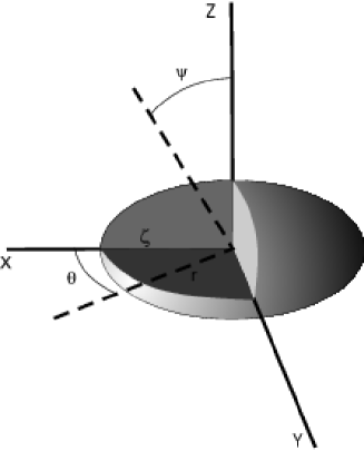
Figure 1: A surface of constant density for the triaxial ellipsoid described in Eq. (5) and (6).

The mass models considered in this study are the triaxial generalizations of the spherical models discussed in detail by Ciotti (1991). The mathematical singularities present in Eq. 3 were considered and solved by Simonneau & Prada (1999, Eq. 16). Substituting Eq. 1 into Eq. 3, letting $\xi=\zeta\cosh\varphi$, and multiplying by the mass–to–light ratio $\Upsilon\equiv$M/L, we obtain a similar expression to the one found by these authors:

$$\rho(\zeta)=\frac{f^{1/2}I(0)b_{n}}{\pi nr_{e}^{1/n}}\Upsilon\int_{0}^{\infty}e^{-b_{n}\left(\frac{\zeta\cosh\varphi}{r_{e}}\right)^{1/n}}(\zeta\cosh\varphi)^{1/n-1}d\varphi,$$ (5)

with

$$x^{2}+\left(\frac{y}{\alpha}\right)^{2}+\left(\frac{z}{\beta}\right)^{2}=\zeta^{2}.$$ (6)

The dimensionless mass density profiles $\widetilde{\rho}(\zeta)\equiv r_{e}^{3}/M\rho(\zeta)$, where $M$ is the total mass, are shown for different values of $n$ in Fig. 2a. It should be noted that the inner density profile decreases more slowly with increasing radius for systems having lower values of $n$.

The mass density profiles of the $r^{1/n}$ family (Eq. 5) can be extremely well approximated by the analytical expression:

$$\rho_{app}(\zeta)=\frac{f^{1/2}I(0)b_{n}2^{(n-1)/2n}}{r_{e}n\pi}\Upsilon\frac{h^{p(1/n-1)}K_{\nu}(b_{n}h^{1/n})}{1-C(h)},$$ (7)

where $h=\zeta/r_{e}$, $C(h)=h_{1}(\log h)^{2}+h_{2}\log h+h_{3}$ and $K_{\nu}$ is the $\nu$th–order modified Bessel function of the third kind (Abramowitz & Stegun 1964, p. 374). In the Appendix A we show the values of the parameters ($\nu$,p,h₁,h₂,h₃) as function of the index $n$. This approximation contains two exact cases: $n$=0.5 and $n$=1, and provides relative error less than 0.1% for the rest of the cases (Fig 2b) in the radial range 10${}^{-3}\leq\zeta/r_{e}\leq 10^{3}$. This approximation surpasses (by a factor of 10²–10⁴) the expression presented in Lima Neto, Gerbal & Márquez (1999).

Figure 2: a) The dimensionless mass density profiles (see Section 2.1) for the values of $n$=0.5, 1, 2, 4 and 10. b) the relative error between the the analytical approximation proposed in Eq. 7 and the exact solution are shown for the previous values of $n$.

3 Non–axisymmetric perturbations due to a triaxial $r^{1/n}$ structure

For three different triaxiality mass distributions: a) spherical ($\alpha$=$\beta$=1); b) moderately triaxial ($\alpha$=0.75, $\beta$=0.5); c) highly triaxial ($\alpha$=0.5, $\beta$=0.25), we have explored, in detail, the non–axisymmetric gravitational field over the z=0 plane (i.e. the disc plane when studying spiral galaxies).

3.1 Non–spherical component of the gravitational potential in the plane z=0

We evaluate this quantity by calculating:

$$G(r)\equiv\frac{\Phi_{2}(r)}{\Phi_{0}(r)},$$ (8)

where $\Phi_{2}(r)$ and $\Phi_{0}(r)$ are the m=2 and m=0 component of the gravitational potential, such that the nth–order term $\Phi_{m}(r)$ is evaluated from the gravitational potential on the z=0 plane $\Phi(r,\theta)$ by using the Fourier decomposition (see, e.g. Combes & Sanders 1981). Gravitational potential and gravitational force expressions are shown on Appendix B.

The profiles of $G(r)$ for different triaxialities and values of $n$ are shown in Fig. 3. As it is expected, as the triaxiality increases the non–spherical nature of the gravitational field increases. Also, we highlight that for a given triaxiality, smaller values of $n$ (i.e less concentrated mass distribution) give greater non-spherical gravitational fields. The maximum non–axisymmetrical behavior of the potential is obtained at radial distances less than 2 $r_{e}$. This radial distance is also a function of the index $n$, decreasing a $n$ increases and remains quite independent of the triaxiality of the object. For a moderately triaxial object with $n$=1, the non–axisymmetrical component of the potential can vary some 6% between r=0 and r=2$r_{e}$, and varies some 15% for our highly triaxial model.

For an $n$=1 model, and starting from our moderately triaxial case ($\alpha$=0.75, $\beta$=0.50), we increased the value of $\beta$ to 0.75. The results are shown in Fig. 3c and reveal that G(r) varied only mildly. This figure shows that the non–axisymmetric effect (along the radial distance) in the z=0 plane is mainly due to how the mass of the bulge is distributed in this plane.

3.2 Non–spherical component of radial gravitational forces in the z=0 plane

The non–spherical component of the radial gravitational forces in the z=0 can be estimated by:

$$N(r)\equiv\frac{\partial\Phi_{2}(r)/\partial r}{\partial\Phi_{0}(r)/\partial r}.$$ (9)

In Fig. 3 the N(r) profiles (Eq. 9) are evaluated for the same cases as was the G(r) profiles. A remarkable point is that N(r) reaches its maximum value in the radial range 2 $r_{e}$$<$r$<$4 $r_{e}$. For a spiral bulge structure, this means that the most important non–axisymmetric effects take place in a zone which is dominated by the disc. As with the G(r) parameter, stronger distortions occur as the triaxiality increases and the index $n$ decreases. The mechanism which controls this distortion is basically determined by the mass distribution in the z=0 plane (Fig 3c).

It is noted that the relative (i.e. % change) non–axisymmetric effects on the radial forces are larger than the relative distortion on the potential. As an example, for a moderately triaxial structure with $n$=1 the non–axisymmetric component of the radial forces can reach 8%.

3.3 Torques on z=0 plane

The torques provoked by the triaxial structures along the angular coordinate are evaluated around the circle of radius $r_{max}$ where the maximum non–axisymmetrical distortion of the radial forces is produced (i.e. at the peak of the N(r) profile). Given the gravitational potential $\Phi(r,\theta)$ in the z=0 plane, we have at the radius $r_{max}$:

$$\Pi(\theta)\equiv\frac{F_{T}(r_{max})}{F_{R}(r_{max})},$$ (10)

where $F_{T}(r_{max})=[\partial\Phi(r_{max},\theta)/\partial\theta]/r_{max}$ represents the amplitude of the tangential force along the angular coordinate at radius $r_{max}$, and $F_{R}(r_{max})=(\partial\Phi(r_{max},\theta)/\partial r)$ is the radial force at this radius. Due to the symmetry of the ellipsoid, the values of $\Pi(\theta)$ need only be plotted for one quadrant in the z=0 plane; we use 0^∘$<\theta<$90^∘ (Fig. 3). Depending on the quadrant, $\Pi(\theta)$ is either negative or positive because the sign of the tangential force changes from quadrant to quadrant. The maximum torque around a circle of radius $r_{max}$ depends on the triaxiality of the object. As the triaxiality increases the maximum torque tends to be closer to the major axis – as one would expect. The position of this peak is quite independent of the value of $n$.

The absolute value of the torque for any given triaxiality increases as $n$ decreases. For our highly triaxial bulge, $\Pi(\theta)$ ranges from 0.17 ($n$=10) to 0.24 ($n$=1), which would be considered a ”bar strength” class of 2 in the classification scheme of Buta & Block (2001). In the case of our moderately triaxial object, the maximum absolute value of $\Pi(\theta)$ ranges between 0.06 and 0.09. These values correspond to a “bar strength” class of 1. Thus, even a moderately triaxial bulge is capable of provoking non–negligible torques on a disk – that is to say, a bar is not neccessarily required. A detailed study separating the torque contribution from both bars and bulges would of course be of interest, and it is our intention to add a range of bar potentials to our models in the future.

As with the previous parameters, for the range of triaxialities investigated and a given $n$, varying the mass distribution along the z–axis (i.e. varying the triaxiality parameter $\beta$) only results in a slight change to $\Pi(\theta)$ (see Fig. 3c). For a spherical distribution all above parameters are 0.

Figure 3: The parameters G(r), N(r) and $\Pi(\theta)$ are shown for different values of $n$ and triaxiality: a) First Row: G(r), N(r) and $\Pi(\theta)$ for a moderately triaxial object and different $n$; b) Second Row: G(r), N(r) and $\Pi(\theta)$ for a highly triaxial structure; c) Third Row: G(r), N(r) and $\Pi(\theta)$ for three moderately triaxial objects with $n$=1 and the same axis ratio along the y and x axis.

4 Linking theory and observations: the connection between n and the B/D luminosity ratio

Figure 4: The best–fitting bulge index $n$ is plotted against the $B/D$ luminosity ratio (left) and versus the galaxy morphological type (right). The galaxies come from the samples of de Jong (1996) (solid points) and Andredakis et al. (1995) (open diamonds). See text for details.

In the previous section we have seen how the non–axisymmetrical effects (in the z=0 plane) from a triaxial bulge increase as $n$ decreases. Taken with the correlation between $n$ and galaxy type (Andredakis, Peletier & Balcells 1995) shown in Fig. 4, this invokes the natural question: How, if at all, are the structural properties of the bulges (i.e. $n$) related (that is, cause and effect) with the non–axisymmetrical components (i.e. arms) observed in the disc? The results obtained in the previous sections were evaluated without any mention to the relative mass of the bulge and disc. It turns out that the axisymmetrical mass distribution of the disc causes a strong softening of the non–axisymmetrical perturbation caused by the non–sphericity of the bulge. The degree of “smoothing” is an increasing function of the $D/B$ ratio.

Fig. 5 shows the N(r) profile for a moderately triaxial bulge with $n=1$ and $B/D$=0.1 and 0.01, and for a bulge with $n=4$ and $B/D$=1.0 and 0.1 (Fig. 4). N(r) was evaluated here assuming the disc follows an exponential surface brightness distribution. The ratio between the length scale of the disc and the effective radius of the bulge is assumed to be constant and with a value of $h/r_{e}$=5 . The expressions for the potential and the radial force of these structures can be found in Binney & Tremaine (1987, p. 77 and 78).

Fig. 5 illustrates that for $B/D$ luminosity ratios typical of real galaxies, the non–axisymmetrical effects on the disc largely disappear ($<3\%$). For $B/D$=1, the values of the N(r) profile remain basically unchanged to that seen in Fig. 3, but for $B/D$=0.1 these values decrease approximately by a factor 2, and for $B/D$=0.01 this factor is bigger than 10. Thus, although the non–radial effects on the z=0 plane increase as $n$ decreases, the smoothing effects of the increasingly dominant disc are stronger. Bulges with small values of $n$ are unable to produce significant non–axisymmetrical effects on a massive disc.

Figure 5: The N(r) profiles for a moderately triaxial bulge with $n$=1 and 4, and $B/D$=1, 0.1, 0.01 are shown.

4.1 Why does the $n$–$Type$ (or $n$–$B/D$) relation exist?

To explore the connection between bulges and discs in spiral galaxies (see, e.g. Fuchs 2000), we have used the data from two independent samples of galaxies observed in the K–band. The K–band provides a good tracer of the mass due to the near absence of dust extinction and the reduced biasing effect of a few per cent (in mass) of young stars. We used the data from Andredakis et al. (1995) and the structural analysis of the de Jong (1996) data performed by Graham (2001). Both studies were done fitting a seeing convolved Sérsic law to the spiral galaxy bulges. In both samples we have removed those objects which contained a clear bar structure, leaving a total of 28 objects from Andredakis et al. (1995) and 52 objects from Graham (2001). The relations present in Fig. 4 between $n$ and the $B/D$ luminosity ratio, and $n$ versus the morphological type T have a Spearman rank–order correlation coefficient of $r_{s}=0.77$ and $r_{s}=-0.73$, respectively, for the combined sample.

Andredakis et al. (1995) suggest “although other possibilities cannot be excluded, the most straightforward explanation for this trend is that the presence of the disc affects the density distribution of the bulge in such a way as to make the bulge profile steeper in the outer parts. One mechanism to produce such an effect might be that a stronger disc truncates the bulge, forcing its profile to become exponential”. Following this line of thought, via collisionless N–body simulations, Andredakis (1998) studied the adiabatic growth of the disc onto an existing $r^{1/4}$ spheroid. He found that the disc potential modifies the bulge surface brightness profile, lowering the index $n$. This decrease was larger with more massive and more compact discs. This mechanism, however, saturated at around $n$=2 and exponential bulges could not be produced.

We believe that this line of reasoning is not the most appropiate explanation for the relation between $n$ and $B/D$. Firstly, we find that the index $n$ is not only well correlated with the luminous $B/D$ ratio, but is equally well correlated ($r_{s}=-0.75$) with bulge luminosity $M_{K_{T}}(bulge)$ (Fig. 6a). Additionally, the correlation between $n$ and disc luminosity $M_{K_{T}}(disc)$ is relatively poor ($r_{s}=-0.53$). Secondly, $M_{K_{T}}(bulge)$ is more strongly correlated ($r_{s}=-0.86$) with the $B/D$ ratio than $M_{K_{T}}(disc)$ and the $B/D$ ratio ($r_{s}=-0.50$) (Fig. 6b). Hence, it is variations in the bulge which are predominantly responsible for variations in the $B/D$ ratio.

These above two correlations seem to indicate that $n$ may be related directly with the properties of the bulge rather than with the combined $B/D$ ratio. Consequently, as $n$ is correlated with the total bulge luminosity, the correlation between $n$ and $B/D$ is a result of the more fundamental correlation between $M_{K_{T}}(bulge)$ and $B/D$. That is, it is not the relative increase in disc–to–bulge luminosity which produces bulges with smaller values of $n$, but simply that bulges with larger values of $n$ are more luminous (or vice–versa) and this produces the correlation between $n$ and the $B/D$ luminosity ratio.

Favouring this argument, we note that among the Elliptical galaxies (without the need to invoke any disc) there exists a strong correlation (Pearson’s r=-0.82; Graham, Trujillo & Caon, 2001) between $n$ and the total luminosity of these objects. The index $n$ of pressure supported stellar systems are related with the total luminosity of these structures. In agreement with this, Aguerri, Balcells & Peletier (2001) have found (using collisionless N–body simulations) that the bulges of late–type galaxies can increase their $n$ values via dense satellite accretions where the new value of $n$ is found to be proportional to the devoured satellite mass.

Figure 6: a) The absolute K–band magnitude of the bulge (top panel) and the disc (bottom panel) are plotted versus the index $n$. The galaxies come from the samples of de Jong (1996) (solid points) and Andredakis et al. (1995) (open diamonds). See text for details. b) The absolute K–band magnitude of both bulge and disc are shown as a function of the $B/D$ ratio. The galaxies come from the samples of de Jong (1996) (solid points) and Andredakis et al. (1995) (open diamonds). See text for details.

4.2 $M_{K_{T}}(bulge)$ versus $B/D$ for classifying morphological types

Due to the strong correlation between the $B/D$ luminosity ratio and $M_{K_{T}}(bulge)$, it might be of interest to ask which one of these quantities is preferred to establish the morphological type T of a galaxy. Working from B–band images (which is good for observing the young star population, and consequently the spiral arm structure, which is one of the basic criteria to the Hubble galaxy classification), Simien & de Vaucouleurs (1986) fitted $r^{1/4}$ profiles and exponential discs to a sample of 64 spiral galaxies and 34 S0 type galaxies. They presented a good correlation between the bulge–to–disc luminosity and $T$, but not between $M_{B_{T}}(bulge)$ and $T$. Consequently, their B–band observations suggested that the $B/D$ luminosity ratio was preferred to $M_{B_{T}}(bulge)$ for establishing the morphological type T. In Fig. 7 we show the relation between the $B/D$ luminosity ratio and T ($r_{s}=-0.65$) and between $M_{K_{T}}(bulge)$ and T ($r_{s}=0.67$). Thus, from K–band observations, and fitting $r^{1/n}$ bulge profile models, the change in the luminous mass of the bulge along the Hubble sequence appears equally as important as the combined change in the bulge and disc luminosity. It would then follow that the luminous mass of the bulge (i.e. $M_{K_{T}}(bulge)$) is related with the spiral arm structure.

Figure 7: The K–band $B/D$ ratio and the absolute K–band magnitude of the bulge are shown as a function of the morphological type. The galaxies come from the samples of de Jong (1996) (solid points) and Andredakis et al. (1995) (open diamonds). See text for details.

5 conclusions

The main results of this work are the following:

a) We have generalised the analysis of the physical properties of spherical stellar systems following the $r^{1/n}$ luminosity law to a homologous triaxial distribution. The density distribution, potential, forces and torques are evaluated and compared with the spherical case when applicable (Ciotti 1991). An extremely accurate analytical approximation (relative error less than 0.1%) for the mass density profile is provided.

b) We derive an exact expression showing how the central potential decreases as triaxiality increases. We also show that for a fixed triaxiality, as the index $n$ decreases the non–axisymmetrical effects in the z=0 plane increase. Even for a moderately triaxial object, the non–axisymmetrical component of the potential and the radial forces are not negligible for small values of $n$. These components can range from 6 to 8%, respectively, compared to the value of the spherical component. For our highly triaxial model, they can range over some 20%.

c) The non–axisymmetrical effects in the disc plane due to the bulge structure are strongly reduced when an axisymmetrical disc mass is added. For this reason, bulges with smaller values of $n$ appear unlikely to produce any significant non–axisymmetrical effect on their disc, which is typically 10 to 100 more times more massive than the bulge. In this regard, the $B/D$ mass ratio and the triaxiality of the bulge are more important, that is, can dominate over the effects of small $n$.

d) The correlation found between $n$ and the $B/D$ luminosity ratio found in spiral galaxies is explained here not as a consequence of the interplay between the bulge and the disc, but due to the strong correlation between $n$ and $M_{T}(bulge)$, and between $M_{T}(bulge)$ and $B/D$. Also, K–band data do not support the idea that the $B/D$ luminosity ratio can be preferred over $M_{T}(bulge)$ as an indicator to establish galaxy morphological type (T). Both parameters present equally good correlations with galaxy type T.

Appendix A Mass density approximation parameters

The table A1 shows the values of the parameters that appear in the mass density approximation (Eq. 7).

Table 1: Parameter values of the mass density approximation

$n$	$\nu$	p	h1	h2	h3	Max. Rel. Error (%)
0.5	-0.50000	1.00000	0.00000	0.00000	0.00000	0.000
1.0	0.00000	0.00000	0.00000	0.00000	0.00000	0.000
1.5	0.43675	0.61007	-0.07257	-0.20048	0.01647	0.100
2.0	0.47773	0.77491	-0.04963	-0.15556	0.08284	0.070
2.5	0.49231	0.84071	-0.03313	-0.12070	0.14390	0.070
3.0	0.49316	0.87689	-0.02282	-0.09611	0.19680	0.060
3.5	0.49280	0.89914	-0.01648	-0.07919	0.24168	0.050
4.0	0.50325	0.91365	-0.01248	-0.06747	0.27969	0.020
4.5	0.51140	0.92449	-0.00970	-0.05829	0.31280	0.020
5.0	0.52169	0.93279	-0.00773	-0.05106	0.34181	0.015
6.0	0.55823	0.94451	-0.00522	-0.04060	0.39002	0.005
7.0	0.58086	0.95289	-0.00369	-0.03311	0.42942	0.005
8.0	0.60463	0.95904	-0.00272	-0.02768	0.46208	0.004
9.0	0.61483	0.96385	-0.00206	-0.02353	0.48997	0.004
10.0	0.66995	0.96731	-0.00164	-0.02053	0.51325	0.005

Appendix B Gravitational potential and forces of a triaxial homologous structure

B.1 Gravitational Potential

The gravitational potential at position ${\bf x}=(x,y,z)$ may be written as

$$\Phi({\bf x})=\pi Gabc\int_{0}^{\infty}\frac{[\psi(a)-\psi(\zeta)]d\tau}{\sqrt{(\tau+a^{2})(\tau+b^{2})(\tau+c^{2})}}$$ (11)

(Chandrasekhar 1969, p. 52, theorem 12), with

$$\psi(\zeta)=\frac{2}{a^{2}}\int_{a}^{\zeta}\zeta^{{}^{\prime}}\rho(\zeta^{{}^{\prime}})d\zeta^{{}^{\prime}}.$$ (12)

It follows from Eq. (B1) that the potential at an internal point is a result of two contributions: that due to the ellipsoid interior to the point ${\bf x}$ considered, and that due to the homoeoidal shell exterior to ${\bf x}$:

$$\Phi({\bf x})=4\pi G\alpha\beta\frac{1}{\sqrt{1-\beta^{2}}}$$ (13)

$$\Bigg{[}F\left(\arcsin\sqrt{1-\beta^{2}},\sqrt{\frac{1-\alpha^{2}}{1-\beta^{2}}}\right)\int_{\zeta}^{\infty}\zeta^{{}^{\prime}}\rho(\zeta^{{}^{\prime}})d\zeta^{{}^{\prime}}+$$

$$\int_{0}^{\zeta}\zeta^{{}^{\prime}}\rho(\zeta^{{}^{\prime}})F\left(\arcsin\sqrt{\frac{(1-\beta^{2})\zeta^{{}^{\prime}2}}{\zeta^{{}^{\prime}2}+\lambda}},\sqrt{\frac{1-\alpha^{2}}{1-\beta^{2}}}\right)d\zeta^{{}^{\prime}}\Bigg{]},$$

with F(p,q) the Elliptic integral of the first kind (Abramowitz & Stegun 1964, p. 589), and with the restriction

$$\frac{x^{2}}{\zeta^{{}^{\prime}2}+\lambda}+\frac{y^{2}}{(\zeta^{{}^{\prime}}\alpha)^{2}+\lambda}+\frac{z^{2}}{(\zeta^{{}^{\prime}}\beta)^{2}+\lambda}=1.$$ (14)

The strength of the central potential decreases as the triaxiality of the object increases:

$$\frac{\Phi(0)}{\Phi_{sph}(0)}=\frac{f^{1/2}\alpha\beta}{\sqrt{1-\beta^{2}}}F\left(\arcsin\sqrt{1-\beta^{2}},\sqrt{\frac{1-\alpha^{2}}{1-\beta^{2}}}\right).$$ (15)

As reported in Ciotti (1991), the models with low $n$ have an inner ($r<r_{e}$) potential which is much flatter than models with high $n$. As the triaxiality increases there is no important change to the gradient of the gravitational potential along the semimajor–axis; the main effect is to shift the gravitational potential profile inwards from the spherical case, resulting in a lower potential at intermediate radii.

B.2 Gravitational Forces

The gravitational forces for a triaxial structure are given by the expression:

$$-\frac{\partial\Phi({\bf x})}{\partial x_{i}}=4\pi G\alpha\beta x_{i}$$ (16)

$$\int_{0}^{\zeta}\frac{1}{(\zeta^{{}^{\prime}}a_{i}/a)^{2}+\lambda}\frac{\zeta^{{}^{\prime}2}\rho(\zeta^{{}^{\prime}})}{\sqrt{(\zeta^{{}^{\prime}2}+\lambda)((\alpha\zeta^{{}^{\prime}})^{2}+\lambda)((\beta\zeta^{{}^{\prime}})^{2}+\lambda)}}\frac{d\zeta^{{}^{\prime}}}{f(\zeta^{{}^{\prime}},a_{i})},$$

$$i=1,2,3$$

with $a_{1}\equiv$ a, $a_{2}\equiv$ b, $a_{3}\equiv$ c, and

$$f(\zeta^{{}^{\prime}},a_{i})=\sum_{i=1,2,3}\frac{x_{i}^{2}}{\left[(\zeta^{{}^{\prime}}a_{i}/a)^{2}+\lambda\right]^{2}}.$$ (17)

The restrictions given in Eqs. (6) and (B4) also apply here.

References

- [1] Abramowitz M., Stegun I., 1964, Handbook of Mathematical Functions. Dover, New York
- [2] Aguerri, J.A.L., Balcells M., Peletier R., 2001, A&A, 367, 428
- [3] Andredakis Y.C., Peletier R., Balcells M., 1995, MNRAS, 275, 874
- [4] Andredakis, Y.C., 1998, MNRAS, 295, 72
- [5] Binney, J., Tremaine, S.: 1987, Galactic Dynamics, Princeton University Press, Princenton
- [6] Buta R., & Block D.L., 2001, ApJ, 550, 243
- [7] Block, D.L., Puerari, I., Frogel J.A., Eskridge, P.B., Stockton A., Burkhard F., 1999, Astroph. and Space Sci, 269–270, 5
- [8] Caon N., Capaccioli M., D’Onofrio M., 1993, MNRAS, 265, 1013
- [9] Capaccioli M., 1987, in Structure and Dynamics of Elliptical Galaxies, IAU Symp. 127, Reidel, Dordrecht, p.47
- [10] Capaccioli M., 1989, in The World of Galaxies, ed. H. G. Corwin, L. Bottinelli (Berlin: Springer-Verlag), p.208
- [11] Chakraborty D. K. & Thakur P., 2000, MNRAS, 318, 1273
- [12] Chandrasekhar, S. 1969, Ellipsoidal Figures of Equilibrium (New York: Dover)
- [13] Ciotti, L. 1991, A&A, 249, 99
- [14] Combes, F., & Sanders, R.H. 1981, A&A, 96, 164
- [15] Davies J., Philips S., Cawson M., Disney M., Kibblewhite E., 1988, MNRAS, 232, 239
- [16] Dehnen, W., 1993, MNRAS, 265, 250
- [17] de Jong, R.S., 1996, A&AS, 118, 557
- [18] de Vaucouleurs G., 1948, Ann. Astrophys, 11, 247
- [19] de Vaucouleurs G., 1959, Hand. Phys., Vol. 53, p. 311
- [20] Fuchs, B., 2000, in: F. Combes and G. Mamon (eds.), Galaxy Dynamics: from the Early Universe to the Present, ASP Conference Series, Vol. 197
- [21] Graham A.W., Lauer T., Colles M.M., Postman M., 1996, ApJ, 465, 534
- [22] Graham A.W., Prieto M., 1999, ApJ, 524, L23
- [23] Graham A.W., 2001, AJ, 121, 820
- [24] Graham A.W., Trujillo, I., Caon, N., 2001, AJ, 122, 1707
- [25] Graham A.W., Erwin, P., Caon, N., Trujillo, I., 2001, ApJ, 563, L11
- [26] Hernquist, L., 1990, ApJ, 356, 359
- [27] Jaffe, W., 1983, MNRAS, 202, 995
- [28] Jerjen, E., Bingelli, B. 1997, in the Nature of Elliptical Galaxies; The Second Stromlo Symposium, ASP Conf. Ser., 116, 239
- [29] Khosroshahi H.G., Wadadekar Y., Kembhavi A., 2000, ApJ, 533, 162
- [30] Lima Neto G. B., Gerbal D. & Márquez I., 1999, MNRAS, 309, 481
- [31] Mazure A. & Capelato H.V. 2002, A&A, in press
- [32] Möllenhoff C., Heidt J., 2001, A&A, 368, 16
- [33] Moriondo G., Giovanardi C., Hunt L.K., 1998, A&AS, 130, 81
- [34] Prieto, M., Aguerri, J.A.L., Varela, A.M. & Munoz-Tunon, C., 2001, A&A, 367, 405
- [35] Sandage, A., 1961. The Hubble atlas of galaxies, Washington: Carnegie Institution
- [36] Seigar, M. & James, P., 1998, MNRAS, 299, 672
- [37] Sèrsic J. 1968. Atlas de Galaxias Australes Córdoba: Obs. Astronómico
- [38] Simien, F., de Vaucouleurs, G., 1986, ApJ, 302, 564
- [39] Simonneau E., Varela A., Muñoz–Tuñoz C., 1998, Il Nuovo Cimento, 113B, 927
- [40] Simonneau E., Prada F., 1999, (astro–ph/9906151)
- [41] Stark A., 1977, ApJ, 213, 368
- [42] Trujillo, I., Aguerri, J.A.L., Cepa, J., Gutierrez, C.M., 2001, MNRAS, 321, 269
- [43] Trujillo, I., Graham, A.W., Caon, N., 2001, MNRAS, 326, 869
- [44] Varela A., Muñoz–Tuñoz C., Simonneau E., 1996, A&A, 306, 381
- [45] Young, C.K., Currie, M.J., 1994, MNRAS, 268, L11
- [46] Young, C.K., Currie, M.J., 1995, MNRAS, 273, 1141
- [47] Zhao H., 1997, MNRAS, 287, 525