Wind Accretion and Binary Evolution of the Microquasar LS 5039

Abstract

There is much evidence to suggest that stellar wind capture, rather than Roche lobe overflow, serves as the accretion mechanism onto the compact secondary object in the massive X-ray binary LS 5039. The lack of significant emission combined with only a modest X-ray flux provide observational evidence that no large-scale mass transfer is occurring (consistent with our estimate of the radius of the O6.5 V((f)) optical star that is smaller than its critical Roche radius). Here we determine the mass loss rate of the optical star from the broad, residual emission in the H$\alpha$ profile. Using a stellar wind accretion model for a range in assumed primary mass, we compute the predicted X-ray luminosity for the system. We compare our results to the observed X-ray luminosity to determine the mass of the compact object for each case. The companion appears to be a neutron star with a mass between 1 and $3M_{\odot}$. With our new constraints on the masses of both components, we discuss their implications on the evolution of the system before and after the supernova event that created the compact companion. The binary experienced significant mass loss during the supernova, and we find that the predictions for the resulting runaway velocity agree well with the observed peculiar space velocity. LS 5039 may be the fastest runaway object among known massive X-ray binaries.

1 Introduction

LS 5039 is a relatively faint ($V=11.3$) and massive star of type O6.5 V((f)) (Clark et al., 2001) that is one of only a few confirmed massive X-ray binaries (MXRBs) with associated radio emission (Ribó et al., 1999). It has radio-emitting relativistic jets characteristic of galactic microquasars, and it is probably a high energy gamma ray source as well (Paredes et al., 2000). We recently discovered that the system is a short period binary ($P=4.117\pm 0.011$ d) with the highest known eccentricity ($e=0.41\pm 0.05$) among O star binaries with comparable periods (McSwain et al., 2001a). This high eccentricity probably results from the huge mass loss that occurred with the supernova (SN) explosion that gave birth to the compact star in the system (Bhattacharya & van den Heuvel, 1991; Nelemans et al., 1999). Binaries that suffer large mass loss in a SN are expected to become runaway stars, and recently both we (McSwain et al., 2001b) and Ribó et al. (2002) found that LS 5039 has a relatively large proper motion that indicates that the binary has a record-breaking peculiar space velocity among MXRBs.

Reliable estimates for the masses of the components of the binary are of key importance for any discussion about the evolution of this remarkable system. Here we present an investigation of the possible mass range for the X-ray star based on a stellar wind accretion model for the X-ray production (§2). This analysis relies on our observations of the wind emission effects in the H$\alpha$ profile and the wind models of Puls et al. (1996). We then apply our derived mass estimates for both stars to determine the probable masses and orbital parameters prior to the SN based on the system’s current eccentricity (§3). We find that the predicted and observed runaway velocities are in good agreement, and, thus, LS 5039 provides the best verification to date of model predictions about the outcome of a SN explosion in a massive binary.

2 X-ray Fueling by Wind Accretion

The X-ray production in MXRBs results from mass accretion through a Roche lobe overflow (RLOF) stream or by Bondi-Hoyle accretion from the stellar wind of the luminous primary (Kaper, 1998). The systems experiencing RLOF usually have large X-ray luminosities and striking optical emission lines. However, LS 5039 has a modest X-ray flux (Ribó et al., 1999) and no obvious emission lines (Clark et al., 2001; McSwain et al., 2001a), and we show below that the O-star is probably smaller than its critical Roche surface. Thus, we can safely assume that most of the mass accretion in LS 5039 occurs through capture of the primary’s stellar wind flow.

The wind accretion luminosity of MXRBs depends on the system separation, wind velocity law, mass loss rate, and mass of the accretor (Lamers et al., 1976). If we can estimate these binary and wind parameters from spectroscopy, then the mass of the compact star can be found by comparing the predicted and observed X-ray luminosities, $L_{X}$. Here we present such an analysis based on the mass loss rate derived from our observations of the H$\alpha$ profile (McSwain et al., 2001a). All the parameters needed in this analysis ultimately depend on the assumed mass of the O-star primary that is poorly constrained at the moment. The simplest assumption is that the primary has a mass typical of single stars of its spectral classification, approximately $40M_{\odot}$ (see the mass calibration of Howarth & Prinja (1989) and the study of comparable stars in the young binary, DH Cep, by Penny et al. (1997)). On the other hand, there is evidence that the primaries in MXRBs may be undermassive for their luminosity (Kaper, 2001), and in extreme cases, their mass may be a factor of three lower than the mass derived by comparing their position in the Hertzsprung-Russell diagram with evolutionary tracks. Thus, we show here the results of a wind accretion model for LS 5039 based on a range in assumed primary mass of 10 – $40M_{\odot}$.

Puls et al. (1996) show how the H$\alpha$ profile in O-stars grows from a pure absorption feature to a strong emission line with increasing stellar wind mass loss rate, and they present a scheme to estimate the mass loss rate based on the observed equivalent width, $W_{\lambda}$, of H$\alpha$. We observed the H$\alpha$ line in the spectrum of LS 5039 over three runs in 1998, 1999, and 2000 with the Coude Feed Telescope at Kitt Peak National Observatory (see McSwain et al. (2001a) for details), and we show in Figure 1 the average profile from each run after shifting each spectrum to the rest frame and convolving the 1998 and 2000 spectra to the resolution of the 1999 run ($R=\lambda/\triangle\lambda=4000$). The H$\alpha$ profile appears to be filled in by broad, residual emission that appears as shallow emission peaks in the wings (perhaps also present in the vicinity of He I $\lambda 6678$ and He II $\lambda 6683$). The emission was apparently stronger during the 1998 and 1999 runs, and we compare in Figure 1 these profiles with the deeper absorption observed in 2000 (dotted lines). The net equivalent width over the entire emission and absorption blend was 2.22, 2.15, and 3.10 Å ($\pm 10\%$) for the average profiles from 1998, 1999, and 2000, respectively. We use the mean of these values, 2.49 Å, in the analysis below. We see no evidence in our spectra of variations in the residual emission with orbital phase, and so we can reliably assume that this weak emission forms in the wind of the primary (and not, for example, in a gas stream or accretion disk in which we would observe orbital variations in radial velocity).

We need estimates of the underlying photospheric component of absorption equivalent width, effective temperature, $T_{\rm eff}$, radius, $R_{O}$, and wind velocity law in order to derive a mass loss rate from the observed equivalent widths using the wind models of Puls et al. (1996) (see their Table 7). We adopted the spectral classification calibration of Howarth & Prinja (1989) to estimate $T_{\rm eff}=40.5\pm 2$ kK and $\log g=4.0\pm 0.2$ for the O6.5 V((f)) primary, which is in reasonable agreement with the results from Strömgren photometry by Kilkenny (1993) and with the values of these parameters derived by Puls et al. (1996) for similar stars. The radius, $R_{O}$, follows from $\log g$ and the assumed mass, $M_{O}$. We assumed the wind velocity law usually applied to O-stars: $v(r)=v_{\infty}(1-R_{O}/r)^{\beta}$ with $\beta=0.8$, $v_{\infty}=2.6v_{\rm esc}$, $v_{\rm esc}=(2(1-\Gamma)GM_{O}/R_{O})^{1/2}$, and $\Gamma=2.6\times 10^{-5}(L_{O}/L_{\odot})/(M_{O}/M_{\odot})$ (Howarth & Prinja, 1989; Puls et al., 1996; Lamers & Cassinelli, 1999). The final parameter to be set is the appropriate photospheric absorption equivalent width. Unfortunately, Puls et al. (1996) only give one value of $W_{\lambda}=3.29$ Å that is specified for a model photosphere with $T_{\rm eff}=40$ kK and $\log g=3.7$. While this effective temperature is nearly applicable here, we expect the equivalent width will be larger in our $\log g=4.0$ case since the Stark broadening of the Balmer lines increases with gravity. We used the NLTE models of Auer & Mihalas (1972) to estimate that the H$\alpha$ equivalent width should be $10\%$ stronger at $\log g=4.0$ compared to $\log g=3.7$ (for $T_{\rm eff}=40$ kK), and we pro-rated accordingly the photospheric equivalent width given by Puls et al. (1996). Our derived estimates of $R_{O}$, $v_{\infty}$, and mass loss rate $\log\dot{M}$ are given for several assumed values of $M_{O}$ in Table 1. The mass loss rate values are close to the average found for O6.5 V stars by Howarth & Prinja (1989), $\log\dot{M}=-6.3$ (in units of $M_{\odot}$ y^-1).

We next calculated the predicted X-ray luminosity for a range in assumed secondary mass, $M_{X}$, using the wind accretion model of Lamers et al. (1976) (using the wind velocity law noted above). Their expression for the X-ray accretion luminosity is

$$L_{X}=(3\times 10^{13}L_{\odot})~{}\zeta S_{a}M_{X}/M_{\odot}$$

where the efficiency factor for the conversion of accreted matter to X-ray flux is $\zeta\approx 0.1$. The accretion rate is

$$S_{a}=\pi r_{a}^{2}\dot{M}/(4\pi a^{2})$$

for a separation $a$ and an accretion radius

$$r_{a}=2GM_{X}/v_{\rm rel}^{2}$$

where $v_{\rm rel}$ is the flow velocity of the wind relative to the accreting star (see their eq. 10a). Given the two assumed masses and the known period, we determined the time-averaged separation of the binary and then calculated $L_{X}$ using our estimates of the wind speed and mass loss rate from above. A sample result is shown in Figure 2 for the average and extreme values of the derived mass loss rate (from the 1999 and 2000 H$\alpha$ equivalent widths) for a test primary mass of $M_{O}=25M_{\odot}$.

The observed value of $L_{X}$ depends on the assumed distance. We used the magnitude $V=11.35\pm 0.1$ and reddening $E(B-V)=1.2\pm 0.1$ from Clark et al. (2001), and then estimated the star’s angular diameter by comparing the unreddened magnitude with model magnitudes from Kurucz (1994) for the adopted $T_{\rm eff}$ and $\log g$ (calibrated with the fundamental $T_{\rm eff}$ data of Code et al. (1976)). The distance is then found from the working value of the stellar radius, $d=0.32~{}R_{O}/R_{\odot}$ kpc. The observed X-ray luminosity was adjusted from the measurements of Ribó et al. (1999) who assumed a distance of 3.1 kpc. This prorated estimate of $L_{X}$ is shown as the shaded region in Figure 2. The estimated mass of the secondary is found where the predicted wind accretion luminosity matches the observed $L_{X}$.

We repeated the wind accretion calculation for a grid of assumed O-star masses, and our final results are listed in Table 1 and plotted in a mass diagram in Figure 3. The results are relatively insensitive to our assumptions about $T_{\rm eff}$ and $\log g$. We found, for example, that models made using $\log g=3.7$ led to lower mass loss rates but also lower wind velocities, so that the wind accretion rates changed very little. Because the slope $dL_{X}/dM_{X}$ is relatively large (see Fig. 2), the details of the accretion model (for example, the value of the efficiency parameter, $\zeta$) do not greatly affect the implied secondary masses. In fact, the largest uncertainty in the results comes from the variation in H$\alpha$ equivalent width between observing runs, which presumably reflects significant changes in the stellar wind mass loss rate. Table 1 also lists the size of the Roche radius at periastron, and we find that the O-star fits comfortably within its Roche lobe over the full range in assumed mass. Our results indicate that the secondary has a mass between 1 and $3M_{\odot}$ (based on the extremes of the observed H$\alpha$ equivalent width and adopted primary mass range), and, thus, the secondary is probably a neutron star.

3 A Supernova in a Binary

The catastrophe of a SN explosion in a massive binary has two immediate consequences. First, the system acquires a large eccentricity that is directly related to the amount of mass lost in the SN event. The periastron separation in the altered orbit corresponds to the pre-supernova semi-major axis. Second, by conservation of momentum, we expect the entire system to attain a runaway velocity that again depends on the mass lost in the SN. We demonstrate here that the values of the observed eccentricity and the probable masses derived above indicate that a huge amount of mass was lost in the SN event that formed LS 5039.

We can use the observed eccentricity to relate the pre- and post-SN orbital parameters if we make the following reasonable assumptions: (1) the pre-SN orbit was circular (almost certainly the case for such a short period and evolved system), (2) any kick velocity imparted to the remnant core due to asymmetries in the explosion was relatively small (Nelemans et al., 1999), (3) the primary suffered only minor ablation of mass in the explosion so that its pre- and post-SN mass is the same (Fryxell & Arnett, 1981), and (4) the system has experienced little or no tidal reduction of the orbital eccentricity since the SN event. Bhattacharya & van den Heuvel (1991) and Nelemans et al. (1999) give the expressions required to calculate the pre-SN parameters, and we list in Table 2 the resulting orbital and physical parameters for an eccentricity $e=0.41\pm 0.05$ (McSwain et al., 2001a) and the masses derived in §2. Table 2 gives the pre-SN period, $P^{\rm initial}$, semi-major axis, $a^{\rm initial}$, SN precursor mass, $M_{2}^{\rm initial}$, and the mass lost in the SN, $\triangle M_{2}$.

The first striking result is the large mass loss that occurred in the SN in LS 5039. Some 5 - $17M_{\odot}$ was lost in the explosion, amounting to more than 81% of the precursor’s mass. This is much larger than the typical inferred mass loss fraction of 35% found by Nelemans et al. (1999) for black hole X-ray binaries. The SN precursor had a smaller mass than the primary at the time of the explosion, so the system was not in danger of total disruption (Nelemans et al., 1999).

The pre-SN orbit was very compact and the stars were in close proximity. We list in Table 2 the sizes of the Roche radii in the pre-SN stage. These radii are quite restrictive, and we find that the primary overfills the Roche lobe in the higher mass solutions. However, the current radius $R_{O}$ given in Table 2 may be larger than the radius at the time of the SN if the primary has evolved to a larger size since then. Nevertheless, the secondary’s Roche radius is also quite small, and it is possible that the system was in a contact or over-contact configuration at the time of the SN. Some kind of close interaction must have occurred since by the time of the SN the mass ratio had reversed and the separation had been increasing (Wellstein et al., 2001). Given this evidence of a pre-SN interaction, the observed C deficiency of the primary (McSwain et al., 2001a) probably results from nuclear-processed gas transferred from the SN progenitor. The currently faster than synchronous rotation of the primary (McSwain et al., 2001a) may correspond to the synchronous rate in the shorter period, pre-SN configuration.

Finally, we list in Table 2 the predicted system runaway velocity, $v_{\rm sys}$, based on conservation of momentum (with errors propagated from the uncertainty in the observed eccentricity). The predictions suggest that the system should have a runaway velocity in excess of 100 km s^-1. Although the systemic velocity along the line of sight is unexceptional (McSwain et al., 2001a), the tangential velocity does appear to be large. The system has a proper motion of $\mu_{\alpha}=4.8\pm 2.4$ mas y^-1 and $\mu_{\delta}=-12.2\pm 2.3$ mas y^-1 in the Tycho-2 catalogue (Hog et al., 2000), and Ribó et al. (2002) have recently used optical and radio astrometry to find an improved estimate of $\mu_{\alpha}=4.7\pm 1.1$ mas y^-1 and $\mu_{\delta}=-10.6\pm 1.0$ mas y^-1. We used the latter measurement together with the systemic radial velocity from McSwain et al. (2001a) (adjusted to the velocity offset of the O III $\lambda 5592$ line that presumably forms deep in the photosphere and is less affected by expansion in the atmosphere) to find the peculiar component of space motion, $v_{\rm pec}$ (following the methods described in Berger & Gies (2001)), and this quantity is listed in the final row of Table 2. We find that there is satisfying agreement between the predicted and observed space velocities, especially towards the higher mass range. Note that if the eccentricity had decreased since the the explosion, then the predicted velocities would be lower than the observed velocities, which is contrary to the results in Table 2. This strengthens our assumption that little or no circularization has occurred in LS 5039 since the SN.

The example of LS 5039 provides a strong confirmation of the predictions made about the eccentricity and runaway velocity that result from a SN explosion in a binary, and we find that both the observed eccentricity and peculiar space velocity can be consistently explained by our derived set of pre- and post-SN parameters. On the other hand, the system may be exceptional among MXRBs in the huge amount of mass lost in the SN. Indeed, LS 5039 appears to be the fastest runaway object known among the MXRBs (Kaper, 2001). The example of LS 5039 hints that there are other similar systems with low X-ray luminosity and small radial velocity variations, but this class of “X-ray quiet” SN descendants will be difficult to detect (Garmany et al., 1980).

Figure 1: The average spectrum of LS 5039 after shifting for orbital motion and convolution to the resolution of the 1999 spectra. The 2000 average spectrum is also plotted with the same offsets as the 1998 and 1999 averages (dotted lines) to emphasize the greater residual H$\alpha$ $\lambda 6563$ emission observed in the first two runs.

Figure 2: The predicted X-ray luminosity from wind accretion for an assumed O-star mass of $25M_{\odot}$ and a range of masses for the companion. The solid line illustrates the result for the average mass loss rate calculated for $M_{O}=25M_{\odot}$ ($\log\dot{M}=-6.3$ for mass loss in $M_{\odot}$ y^-1) while the dot-dashed line and dashed line show the results for the strongest and weakest mass loss rates (from the 1999 and 2000 runs, respectively; $\log\dot{M}$ is labelled in each case). The shaded region gives the estimated X-ray luminosity based on a distance of 2.6 kpc (the estimated distance for $M_{O}=25M_{\odot}$) and the observed X-ray fluxes reported by Ribó et al. (1999). The best match occurs for $M_{X}=1.9M_{\odot}$ in this case.

Figure 3: The mass plane diagram for LS 5039 with the constraints from the wind accretion model. The thick, solid line shows the estimated relationship between assumed O-star mass and the mass of the X-ray source. The surrounding shaded regions show how the solutions change if we adopt the higher mass loss rate from the 1999 observations (lower $M_{X}$ required to obtain the same observed X-ray luminosity) or the lower mass loss rate from the 2000 spectra (upper $M_{X}$ limit). Lines of constant orbital inclination are shown as thin, solid lines. The dashed line indicates the lower limit on $M_{X}$ established by the lack of X-ray or optical eclipses (Ribó et al., 1999; Clark et al., 2001).

Table 1: Range in Stellar Parameters

Parameter	$M_{O}=10M_{\odot}$	$M_{O}=20M_{\odot}$	$M_{O}=30M_{\odot}$	$M_{O}=40M_{\odot}$
$R_{O}$ ($R_{\odot}$)	5.2	7.4	9.1	10.5
$v_{\infty}$ (km s-1)	2018	2400	2656	2854
$\log\dot{M}$ ($M_{\odot}$ y-1)	$-6.7$	$-6.4$	$-6.2$	$-6.1$
$M_{X}$ ($M_{\odot}$)	1.2	1.7	2.1	2.4
$R_{O}{\rm(Roche)}$ ($R_{\odot}$)	8.0	10.5	12.2	13.6
$d$ (kpc)	1.7	2.4	2.9	3.3

Table 2: Binary Parameters

Parameter	$M_{O}=10M_{\odot}$	$M_{O}=20M_{\odot}$	$M_{O}=30M_{\odot}$	$M_{O}=40M_{\odot}$
$P^{\rm initial}$ (d)	1.56	1.56	1.56	1.56
$a^{\rm initial}$ ($R_{\odot}$)	14.2	17.7	20.2	22.2
$M_{2}^{\rm initial}$ ($M_{\odot}$)	5.7	10.6	15.2	19.8
$\triangle M_{2}$ ($M_{\odot}$)	4.6	8.9	13.2	17.4
$R_{O}$ ($R_{\odot}$)	5.2	7.4	9.1	10.5
$R_{O}{\rm(Roche)}^{\rm initial}$ ($R_{\odot}$)	6.1	7.7	8.9	9.8
$R_{2}{\rm(Roche)}^{\rm initial}$ ($R_{\odot}$)	4.7	5.8	6.5	7.1
$v_{\rm sys}$ (predicted) (km s-1)	$120\pm 10$	$154\pm 13$	$178\pm 15$	$197\pm 17$
$v_{\rm pec}$ (observed) (km s-1)	$83\pm 13$	$118\pm 17$	$145\pm 21$	$168\pm 24$

Figure 1:

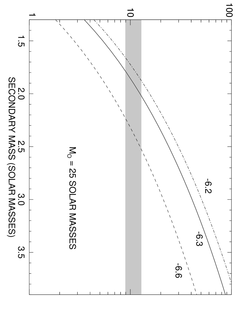
Figure 2:

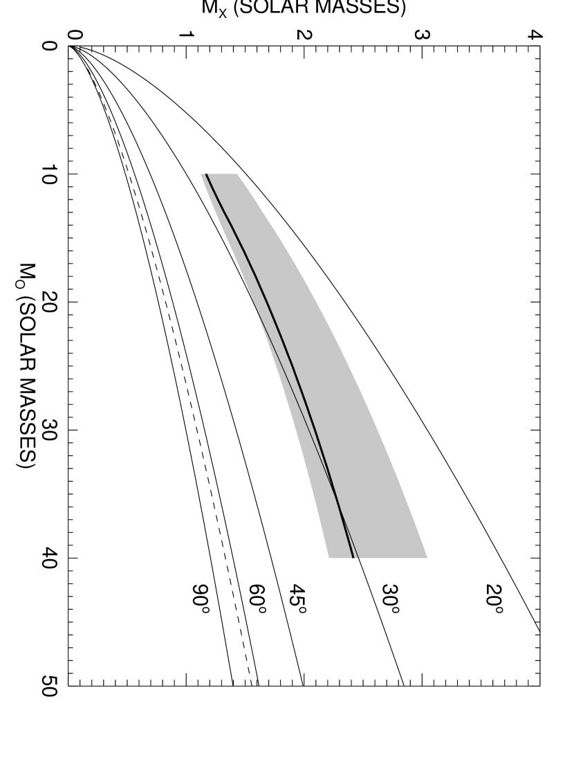
Figure 3:

References

- Auer & Mihalas (1972) Auer, L. H., & Mihalas, D. 1972, ApJS, 24, 193
- Berger & Gies (2001) Berger, D. H., & Gies, D. R. 2001, ApJ, 555, 364
- Bhattacharya & van den Heuvel (1991) Bhattacharya, D., & van den Heuvel, E. P. J. 1991, Physics Rep., 203, 1
- Clark et al. (2001) Clark, J. S., et al. 2001, A&A, 376, 476
- Code et al. (1976) Code, A. D., Bless, R. C., Davis, J., & Brown, R. H. 1976, ApJ, 203, 417
- Fryxell & Arnett (1981) Fryxell, B. A., & Arnett, W. D. 1981, ApJ, 243, 994
- Garmany et al. (1980) Garmany, C. D., Conti, P. S., & Massey, P. 1980, ApJ, 242, 1063
- Hog et al. (2000) Hog, E., et al. 2000, A&A, 355, L27
- Howarth & Prinja (1989) Howarth, I. D., & Prinja, R. K. 1989, ApJS, 69, 527
- Kaper (1998) Kaper, L. 1998, in Boulder-Munich II, Properties of Hot, Luminous Stars (A.S.P. Conf. Ser. 131), ed. I. D. Howarth (San Francisco: A.S.P.), 427
- Kaper (2001) Kaper, L. 2001, in The Influence of Binaries on Stellar Population Studies, ed. D. Vanbeveren (Dordrecht: Kluwer), 125
- Kilkenny (1993) Kilkenny, D. 1993, South African Astron. Obs. Circ., 15, 53
- Kurucz (1994) Kurucz, R. L. 1994, Solar Abundance Model Atmospheres for 0, 1, 2, 4, 8 km/s, Kurucz CD-ROM No. 19 (Cambridge, MA: Smithsonian Astrophysical Obs.)
- Lamers & Cassinelli (1999) Lamers, H. J. G. L. M., & Cassinelli, J. P. 1999, Introduction to Stellar Winds (Cambridge: Cambridge Univ. Press)
- Lamers et al. (1976) Lamers, H. J. G. L. M., van den Heuvel, E. P. J., & Petterson, J. A. 1976, A&A, 49, 327
- McSwain et al. (2001a) McSwain, M. V., Gies, D. R., Riddle, R. L., Wang, Z., & Wingert, D. W. 2001a, ApJ, 558, L43
- McSwain et al. (2001b) McSwain, M. V., Gies, D. R., Riddle, R. L., Wang, Z., & Wingert, D. W. 2001b, AAS Meeting 199, #05.04
- Nelemans et al. (1999) Nelemans, G., Tauris, T. M., & van den Heuvel, E. P. J. 1999, A&A, 352, L87
- Paredes et al. (2000) Paredes, J. M., Martí, J., Ribó, M., & Massi, M. 2000, Science, 288, 2340
- Penny et al. (1997) Penny, L. R., Gies, D. R., & Bagnuolo, W. G., Jr. 1997, ApJ, 483, 439
- Puls et al. (1996) Puls, J., et al. 1996, A&A, 305, 171
- Ribó et al. (2002) Ribó, M., Paredes, J. M., Romero, G. E., Benaglia, P., Martí, J., Fors, O., & García-Sánchez, J. 2002, A&A, in press (astro-ph/0201254)
- Ribó et al. (1999) Ribó, M., Reig, P., Martí, J., & Paredes, J. M. 1999, A&A, 347, 518
- Wellstein et al. (2001) Wellstein, S., Langer, N., & Braun, H. 2001, A&A, 369, 939