ESO Imaging Survey

This paper describes the methodology currently being implemented in the EIS pipeline for analysing optical/infrared multi-colour data. The aim is to identify different classes of objects as well as possible undesirable features associated with the construction of colour catalogues. The classification method used is based on the $\chi^{2}$-fitting of template spectra to the observed SEDs, as measured through broad-band filters. Its main advantage is the simultaneous use of all colours, properly weighted by the photometric errors. In addition, it provides basic information on the properties of the classified objects (e.g. redshift, effective temperature). These characteristics make the $\chi^{2}$-technique ideal for handling large multi-band datasets. The results are compared to the more traditional colour-colour selection and, whenever possible, to model predictions. In order to identify objects with odd colours, either associated with rare populations or to possible problems in the catalogue, outliers are searched for in the multi-dimensional colour space using a nearest-neighbour criterion. Outliers with large $\chi^{2}$-values are individually inspected to further investigate their nature. The tools developed are used for a preliminary analysis of the multi-colour point source catalogue constructed from the optical/infrared imaging data obtained for the Chandra Deep Field South (CDF-S). These data are publicly available, representing the first installment of the ongoing EIS Deep Public Survey.

1 Introduction

The ESO Imaging Survey (EIS) is an ongoing project to carry out public imaging surveys in support of VLT. Its primary goal is to provide multi-wavelength data sets from which samples comprising different types of extragalactic and galactic objects can be extracted for follow-up spectroscopic observations. So far the surveys conducted have used different instrument/telescope setups to carry out moderately deep observations of large areas, deep optical/infrared observations of high-galactic latitude fields, contiguous areas of the SMC and LMC and selected stellar fields including open clusters, and globular clusters (for more details see da Costa, 2001). Altogether over 50 square degrees of the southern sky have already been surveyed, albeit using different filter combinations and reaching different magnitudes (see the EIS web page at “http://www.hq.eso.org/science/eis/”).

The ultimate success of these surveys will, to a large extent, depend on the ability of reliably identifying different classes of objects and extracting well-defined samples for spectroscopic follow-up observations. While colour selection is nothing new and several methods have been devised and applied in the past, the demands of modern, wide-area surveys involving large numbers of objects and passbands is relatively new and must be properly addressed. Therefore, to fully achieve the scientific goals of EIS a detailed understanding of the distribution of objects in colour space is required. This is not only necessary for the selection of spectroscopic targets but also as a verification of the colour catalogues being routinely produced by the survey pipeline.

An ideal way of tackling this problem is to combine intrinsic (e.g. spectral properties) and statistical information (i.e. spatial distribution, luminosity and mass functions, evolution) regarding different classes of known objects. The nature of objects, as characterised by its spectral properties, can be assessed by comparing the measurements obtained from the multi-colour photometry with those estimated using template spectra describing different types of objects. To take into account the statistical properties of a given population requires detailed simulations of the stellar population of our Galaxy as well as the extragalactic populations. These simulations must also satisfy observational constraints, such as sky position, completeness, photometric errors, and morphological classification. In principle, combining these two independent methods should lead to a further improvement of the classification of objects extracted from colour catalogues. As a first step towards this goal, this paper discusses the classification of the objects based exclusively on their spectral properties as derived from multi-colour observations. As a practical illustration, this analysis is applied to the multi-colour point source catalogues extracted from the recently completed optical/infrared data of the Chandra Deep Field South (CDF-S) by the EIS Deep Public Survey (DPS; Vandame et al., 2001; Arnouts et al., 2001a).

The $UBVRI$ optical data covers an area of 0.25 square degrees. These data are complemented by $JK_{s}$ near-infrared observations over 0.1 square degrees located at the centre of the area covered by the optical data. While the angular coverage is relatively small, this is the first complete data set of this survey which at the end will cover a total area of 3 square degrees corresponding to 12 times the data presented here. Therefore the results presented in this paper provide a first assessment of the likely outcome of this survey once completed. Using the CDF-S data as a benchmark is particularly interesting considering the large number of imaging and spectroscopic observations planned for this region, in addition to the already publicly available deep X-ray observations of Chandra (Rosati et al., 2001). These observations will provide an unprecedented multi-wavelength data set that should certainly help refine the classification algorithms being developed.

In Section 2 the data as well as the method employed in the construction of the point source catalogue are briefly reviewed. Section 3 presents the methods used to classify objects based on their colour properties and to search for objects located in poorly populated regions of the colour space. These methods are applied to the CDF-S optical and optical/infrared data and the results are discussed and compared to other methods in Section 4. In this section tables listing different types of objects are also presented. In Section 5 an assessment of the results is carried out by visually inspecting image cutouts and examining the photometric measurements of individual objects to evaluate the performance of catalogue production and target selection procedures. General conclusions and a discussion of the main results is presented in Section 6. Finally, in Section 7 a brief summary is presented.

2 Colour Catalogues

The first step for a target selection from multi-colour data is the construction of multi-colour catalogues. Such catalogues can be produced either by association of objects listed in the single passband catalogues or by building a $\chi^{2}$ image (Szalay et al., 1999) combining the available images in the different passbands. The reference $\chi^{2}$ image is used to detect objects, while their photometric measurements are carried out in the individual single passband images. For the work presented here the first technique has been applied. The $\chi^{2}$ image will be used in future work where a detailed discussion of the pros and cons of the two methods will be presented.

The input to the catalogue association are the single passband catalogues (Vandame et al., 2001; Arnouts et al., 2001a) cut at a $S/N=2$, slightly lower than the catalogues publicly released which were cut at a $S/N$=3. Furthermore, in the present work only objects inside a trimmed region and with appropriate SExtractor flags are considered. Finally, the $U$-band catalogue used here was extracted from an image produced stacking all the available $U/38$ and $U350/60$ images, in order to reach a fainter limiting magnitude. A more detailed discussion of this catalogue and of its photometric calibration will be present in Arnouts et al. (2001b).

After the association, only objects that are in the area common to all catalogues and outside all the masks placed around saturated objects and bright stars, are kept. This ensures that all objects could have been detected in all passbands. An object is included in the final colour catalogue if it is detected with a $S/N\geq$3 in at least one passband. This was done as a compromise between completeness, to avoid pruning possible interesting objects before looking at the data, and the number of spurious detections. If an object is not detected in a particular passband, its magnitude is set to the corresponding 3$\sigma$ limit. Note that the 3$\sigma$ limiting magnitudes (throughout this work all magnitudes are in the Vega system) of the colour catalogues are: $U$=25.7, $B$=27.4, $V$=26.0, $R$=25.9, $I$=24.7, $J$=23.3, and $K_{s}$=21.3.

In the single passband catalogue, point and extended sources are separated using the SExtractor CLASS_STAR flag, up to the morphological classification limit. The point/extended source classification in a colour catalogue is not trivial and the following scheme is adopted. As the point/extended source classification works best for bright objects, the passband utilised for the classification is the one where the object is brightest with respect to the classification limit in that filter (if any). If the object is classified as a point source in this filter, it is considered a point source in the colour catalogue. This procedure is valid as long as the seeing on the images obtained in different passbands is comparable, which is the case here.

The final point-source catalogues considered comprise 1539 and 623 objects in five and seven passbands, respectively. Based on empirical number counts (Wolf et al., 2001a) the completeness of the point-source catalogue is estimated to be $\geq 90$% at $R$=24.5. The present analysis only considers sub-samples consisting of objects detected in at least three bands and those consisting of objects detected only in the red-most passband available over the two regions covered in five and seven filters.

3 Analysis

3.1 Object Classification

Over the years several techniques have been employed to classify objects based on their colour properties, the most common being the selection of objects within regions defined in two-dimensional projections of colour space. These regions are defined based on colour tracks computed from template spectra. While this is a reasonable approach for data sets encompassing a small number of passbands, it is cumbersome to handle photometric errors and as the number of bands increases the problem rapidly becomes untrackable. Furthermore, use of a colour-colour diagram inevitably leads to severe contamination, requires the use of several projections in order to properly constraint a particular population and is not easily implemented for automatic classification for large datasets.

A more suitable approach to handle colour data from large imaging surveys is the $\chi^{2}$-technique (e.g. Wolf et al. 2001b; 2001c) originally developed for galaxy photometric redshift estimation (e.g. Bolzonella et al., 2000 and references therein) and quasar search (Hatziminaoglou et al., 2000, hereafter HMP00; Richards et al., 2001 and references therein). This method is an optimal way of simultaneously handling samples consisting of more than three passbands, reducing the dimensionality of the problem. It consists of fitting the observed spectral energy distribution (SED) of each object to a series of template spectra of different classes of objects, minimising the $\chi^{2}$ given by

$$\chi^{2}=\sum_{i=1}^{n}\frac{(F_{obs}^{i}-F_{mod}^{i}(z))^{2}}{\sigma_{i}^{2}}$$ (1)

$F_{obs}^{i}$ and $F_{mod}^{i}$ are the observed and the template fluxes in the $i$ band, respectively, and $\sigma_{i}$ is the estimated error of the observed flux in this band. The error model adopted includes the error in the magnitudes as estimated by SExtractor added in quadrature to the zero-point error, determined in the photometric calibration of each band. Since SExtractor tends to underestimate the errors for faint sources, their amplitude was corrected to match that estimated from comparisons with external data (e.g. Arnouts et al., 2001a). The above equation is normalised to the passband with the smallest photometric error, although other ways are possible. This subtracts one degree of freedom from the $\chi^{2}$-analysis.

The SED of each object is compared to all available templates separately, and the object is assigned a given type depending on the value of the $\chi^{2}$. Classifications are considered robust (rank 1) if the $\chi^{2}$ is within 95% confidence level; good (rank 2) if in the interval 95-99% and poor (rank 3) if outside the 99% confidence level. Poorly classified objects can indicate an incomplete spectral library, errors in the (theoretical) spectra, inadequacies in the error model adopted and/or undesirable features in the colour catalogue. The reliability of the results, of course, critically depend on the completeness and the quality of the available spectral library. The classification can always be refined by continuously adding measured or improved theoretical spectra. It is important to point out that even if the number of filters is limited to three this approach, in principle equivalent to the traditional colour-colour selection, provides a more convenient way of handling the errors and uses additional constraints based on flux upper-limits.

The spectral library currently in use consists of series of: model quasar, white dwarf and brown dwarf spectra; three empirical cool white dwarf spectra; a set of stellar templates; and a set of model galaxy spectra. The template quasar spectra are assumed to have three different power-law continua (spectral indexes of 0, 0.5 and 1 in the optical). The emission lines (Ly_α, Ly_β, CIII, CIV, MgII, SiIV, H_α, H_β, and H_γ) are assumed to have Gaussian profiles and typical relative intensities and equivalent widths (e.g. Peterson, 1997). The Ly_α forest has been modeled according to Madau (1995). Template spectra were created for redshifts from $z=0$ to $z=6$, in steps of d$z=0.1$. A set of theoretical white dwarf spectra (provided by D. Köster; for the description of the models see Finley et al., 1997; Homeier et al., 1998), with effective temperatures and effective gravities ranging from 6000K to 100000K and $\log g=7-9$, respectively, has been incorporated. Furthermore, three empirical spectra of very cool white dwarves ($T_{\rm eff}<4000$K) have been included, two covering the optical wavelength range (Ibata et al., 2000), and one covering both the optical and near-infrared wavelength range (Oppenheimer et al., 2001). Also included is a series of theoretical low mass stars and brown dwarf spectra (Chabrier et al., 2000) covering temperatures from 500K to 2800K corresponding roughly to masses in the range 0.03 to 0.1 M_⊙, for an effective gravity of $\log g=4.5$. The effective temperature range corresponds approximately to spectral types later than M6V (Kirkpatrick et al., 1991). We should point out that the transition between main sequence M-dwarves and low mass stars is arbitrary, since there is an overlap of templates of objects with temperatures around 2800K. Stellar spectra are taken from the stellar library of Pickles (1998), which contains 131 spectra for a broad range of stellar types (main sequence, giant and sub-giant stars). Finally, the set of galaxy spectra used is the Coleman, Wu & Weedman (1980) model, with no intrinsic evolution. This last set of templates, however, and since this paper only deals with point sources, is only used in cases of poor classifications, as it will be explained later on. The conversion from spectra to magnitudes are carried out using the same response functions as the observations (Vandame et al., 2001; Arnouts et al., 2001a).

It is worth pointing out that a classification scheme based on the $\chi^{2}$-technique may lead to degeneracies, which are type-dependent (e.g. quasars - galaxies - stars). Multiple minima may occur in the parameter space (e.g. redshift - type) and such degeneracies can only be solved by including additional information in the classification procedure. This will be addressed in a forthcoming paper (Hatziminaoglou et al., 2002). In the present work only objects with real detections in at least three passbands are treated. One could also use upper limits as an a posteriori, in order to impose additional constraints and exclude highly improbable solutions. An alternative way is to construct realistic mock catalogues and to combine the colour-space distribution of the different populations with the individual properties (i.e. SED) of the objects (e.g. Hatziminaoglou et al., 2002).

3.2 Searching for Outliers

The technique presented above assumes that all objects belong to classes for which the spectral properties are known. In order not to overlook the presence of unknown populations and to identify possible problems in the process of building the colour sample, it is of great interest to be able to pick up colour-space “outliers”, even though these may simply belong to rare populations, with known spectral properties.

For the systematic identification of outliers the nearest neighbour criterion is adopted using two dissimilarity measures (e.g. Warren et al., 1991). The first measure is the Euclidean distance in colour space given by

$$d_{ii^{\prime},S1}=\sum_{j=1}^{N}(c_{ij}-c_{i^{\prime}j})^{2},$$ (2)

The second is this distance weighted by the photometric errors:

$$d_{ii^{\prime},S2}=\sum_{j=1}^{N}(c_{ij}-c_{i^{\prime}j})^{2}/(\sigma^{2}_{c_{ij}}+\sigma^{2}_{c_{i^{\prime}j}})$$ (3)

where $N$ is the number of possible colours derived from $n$ filters ($N=\frac{n!}{2!(n-2)!}$), $c_{ij}$ the colour $j$ of object i and $\sigma_{c_{ij}}$ the error in the colour. A “nearest-neighbour” criterion is applied next and for each object the $m-th$ smallest value of the respective $d_{ii^{\prime},S1}$ and $d_{ii^{\prime},S2}$ arrays is taken as the degree of isolation of the object from its neighbours (e.g. the stellar locus). In this paper only the cases $m=2$, to search for individual isolated objects, and $m=3$, as an example to isolate different types of objects, are considered. Depending on the characteristics of the survey it might be desirable to use higher values of $m$ to identify possible grouping of rare objects, as originally discussed by Warren et al. (1991). Following these authors, a selection criterion is applied depending on the position of the objects in the d${}_{S_{1}}$ versus d${}_{S_{2}}$ plane, which isolates objects with peculiar colour properties from the rest of the sample. Alternative cluster analysis algorithms are also being examined and will be presented elsewhere.

4 Results

4.1 Quasar Candidates

From the original sample of 1539 objects, morphologically classified as point sources (see Section 2) within the 0.25 square degrees covered in five optical passbands, 1494, detected in at least three filters, were considered. In total there are 204 objects classified as quasars in the magnitude range $19\leavevmode\nobreak\ \hbox to0.0pt{$<$\hss}{\lower 4.30554pt\hbox{$\sim$}}B\leavevmode\nobreak\ \hbox to0.0pt{$<$\hss}{\lower 4.30554pt\hbox{$\sim$}}25$. This number is in excellent agreement with that predicted by quasar models (202${}^{+131}_{-78}$, e.g. Hatziminaoglou et al., 2002) at the limiting magnitude of $B$=25.0, which roughly corresponds to the completeness limit of the colour catalogue considered. It is also in good agreement with estimates based on observed number counts (e.g. Hartwick & Schade 1990; Glazebrook et al., 1995).

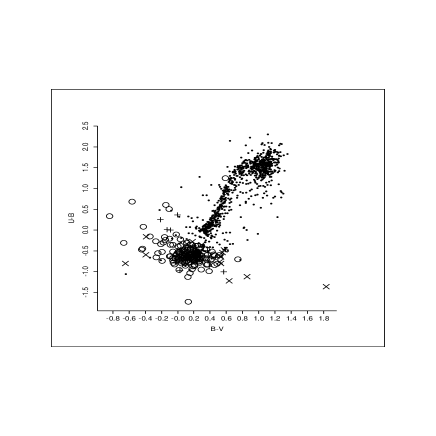
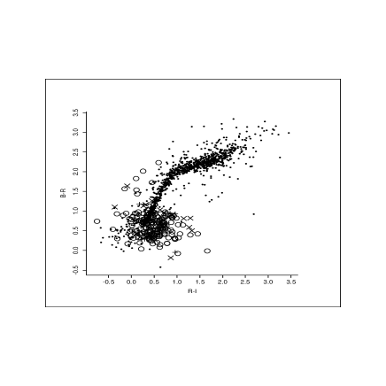
Figure 1: $(U-B)/(B-V)$ (panel (a)) and $(B-R)/(R-I)$ (panel (b)) two-colour diagrams showing the quasar candidates selected on the basis of the $\chi^{2}$-technique. Open circles, plus signs and crosses denote candidates classified at 95%, 95-99% and outside 99% confidence level, respectively.

To help evaluate the results of the $\chi^{2}$-method it is important to compare them with those obtained from a simple colour-colour selection. This is illustrated in Figure 1 which shows the two colour-colour diagrams normally used to identify low to intermediate ($(U-B)/(B-V)$) and high-redshift quasars ($(B-R)/(R-I)$), respectively. In the plot the identified quasars are displayed with different symbols to indicate their associated confidence level as follows: robust (open circles); good (plus signs); and poor (crosses). The same notation applies to all colour-colour plots presented hereafter, unless noted otherwise.

From the careful inspection of these colour-colour diagrams several points can be made regarding the performance of the $\chi^{2}$-analysis. Note, for instance, that nearly all robust candidates are located in the region predicted by the models for low- to intermediate-redshift ($z\leavevmode\nobreak\ \hbox to0.0pt{$<$\hss}{\lower 4.30554pt\hbox{$\sim$}}2.2$) quasars, i.e. $-0.4\leavevmode\nobreak\ \hbox to0.0pt{$<$\hss}{\lower 4.30554pt\hbox{$\sim$}}(B-V)\leavevmode\nobreak\ \hbox to0.0pt{$<$\hss}{\lower 4.30554pt\hbox{$\sim$}}0.7$ and $-1.2\leavevmode\nobreak\ \hbox to0.0pt{$<$\hss}{\lower 4.30554pt\hbox{$\sim$}}(U-B)\leavevmode\nobreak\ \hbox to0.0pt{$<$\hss}{\lower 4.30554pt\hbox{$\sim$}}-0.3$, with a few cases extending into the region where higher redshift quasars are expected to lie. One important short-coming of the standard colour selection is its inability to discriminate between objects with similar colours, leading inevitably to contamination problems. In the particular case of $z\leavevmode\nobreak\ \hbox to0.0pt{$<$\hss}{\lower 4.30554pt\hbox{$\sim$}}2.2$ quasars, the main contaminants are white dwarves and early spectral type main-sequence stars. The results of $\chi^{2}$-analysis suggest that this technique is capable of distinguishing among these different classes, as can been seen from quasar candidates lying very close to and sometimes overlapping objects of other types. Poor candidates are, in general, located at the outskirts of the region delineated by the robust candidates, except for a few cases where the two populations overlap. Similar conclusions can be drawn from the $(B-R)/(R-I)$ diagram shown in panel (b). In particular, given the $B$ filter used, high-redshift quasars ($z\leavevmode\nobreak\ \hbox to0.0pt{$>$\hss}{\lower 4.30554pt\hbox{$\sim$}}3.0$) lie very close to the main sequence, making a colour selection problematic and susceptible to contamination by main-sequence stars. It is worth mentioning the object with $B-V\leavevmode\nobreak\ \sim 1.8$ (see panel (a)) located in a region unlikely to be occupied by quasars. However, on other colour diagrams this object lies close to quasar tracks. A more detailed discussion about its nature will be presented in Section 5.

In order to evaluate the results obtained applying the $\chi^{2}$-method, they can be compared with those based on the more traditional UVX and BRX selection. Adopting criteria similar to those used by Hall et al. (1996) one finds 298 UVX and 49 BRX independent quasar candidates. Out of these, 166 are in common with those classified using the $\chi^{2}$-method. Considering the $\chi^{2}$-classification as reference one estimates a contamination of $\sim 40\%$ in a colour-colour quasar selection, demonstrating the potentiality of the technique for minimising the number of contaminants. Moreover, since it uses the colour information in a combined way, it should also lead to a higher completeness than those based on distances from the stellar locus (e.g. Gaidos, Magnier & Schechter 1993; Newberg & Yanny 1997). For example, colour based selections will tend to miss quasars with redshifts in the range $2.5\leavevmode\nobreak\ \hbox to0.0pt{$<$\hss}{\lower 4.30554pt\hbox{$\sim$}}z\leavevmode\nobreak\ \hbox to0.0pt{$<$\hss}{\lower 4.30554pt\hbox{$\sim$}}3.5$. This is a serious drawback because currently it is believed that the space density of optically-selected quasars starts decreasing in this redshift range. The possible benefits of the $\chi^{2}$-classification over a simple colour selection remains to be evaluated, when spectroscopic data become available.

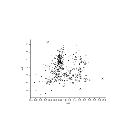
Figure 2: Optical-infrared colour-colour diagram used in the selection of KX candidates, showing the quasar candidates selected on the basis of the $\chi^{2}$-technique. The symbols correspond to those defined in Figure 1.

The CDF-S field has also been observed in the near-infrared $JK_{s}$ passbands over an area of $\sim\leavevmode\nobreak\ 0.1$ square degrees. For this seven passband sub-sample, the number of morphologically classified point sources is 623, out of which 605 are detected in at least three filters. In total there are 92 objects classified as quasar candidates, out of which 62 are in common with those found using only the optical data. The infrared information yields 30 new candidates. Five cases originally classified as quasars are now assigned different classifications: three as white dwarves, one as an G8I and one as a K3I stars.

For the case of optical/infrared all $\chi^{2}$-selected quasar candidates are shown on the $(V-J)/(J-K_{s})$ diagram, introduced by Croom et al. (2001), presented in Figure 2. This diagram is suitable for identifying quasar candidates, due to the following reasons. First, it could partially solve the degeneracy between low to intermediate quasars and white dwarves, occuring when the UVX criterion is applied. Quasars should exhibit a K-excess due to the broad bump created by dust, present in their spectra at the wavelengths around $\sim 1\mu$m (in the rest frame). White dwarves do not have such near-infrared spectral features and should be separated from quasars when the infrared information is added. Second, as pointed out by Croom et al. (2001), KX-selection could identify reddened quasars possibly missed by the UVX selection. Choosing similar regions of colour space as these authors, one finds 65 quasar candidates, 52 of which in common with those UVX selected. Of the KX-selected candidates 34 belong to the quasar candidate list defined using the $\chi^{2}$-technique. From Figure 2 one sees that in order to ensure completeness of $\chi^{2}$-selected robust quasar candidates, one is forced to consider all objects with $V-J<3.0$, which in turn leads to a contamination comparable ($\sim$ 50%) to the one introduced by the UVX selection. Another point worth mentioning is the fact that in Figure 2 one finds red objects not predicted by models of the spectral properties of point-sources. As discussed below, this is probably due to the contamination of the sample by unresolved galaxies (see Section 5). This population is seen in all optical/infrared colour-diagrams presented below.

Another important feature of the the $\chi^{2}$-method is that it can be used not only to classify the objects but also, in the case of extragalactic candidates, to estimate their redshifts. The photometric redshift distribution estimated for the quasar candidate sample selected from the five optical passbands by the $\chi^{2}$-technique is shown in Figure 3, where the three rankings are plotted separately. The distribution covers a broad range of estimated redshifts extending all the way to $z\sim 4.5$. The present sample includes 16 candidates with estimated redshifts $z\leavevmode\nobreak\ \hbox to0.0pt{$>$\hss}{\lower 4.30554pt\hbox{$\sim$}}3.5$, among which 10 are robust classifications. Due to the degeneracy in the assignment of quasar redshifts based solely on broad-band optical filters (HMP00) objects with $z\leavevmode\nobreak\ \hbox to0.0pt{$<$\hss}{\lower 4.30554pt\hbox{$\sim$}}2$ have a considerable dispersion in their estimated photometric redshifts. This accounts for the excess seen at $z\leavevmode\nobreak\ \hbox to0.0pt{$<$\hss}{\lower 4.30554pt\hbox{$\sim$}}0.5$ and the dearth at $1\leavevmode\nobreak\ \hbox to0.0pt{$<$\hss}{\lower 4.30554pt\hbox{$\sim$}}z\leavevmode\nobreak\ \hbox to0.0pt{$<$\hss}{\lower 4.30554pt\hbox{$\sim$}}2$. At $z\sim 1$ there is also the increased probability of misclassifying Compact Emission Line Galaxies (CELGs) as quasar candidates, as shown by HMP00 using the DMS spectroscopic sample. The dearth of objects with redshifts in the interval $2.5\leavevmode\nobreak\ \hbox to0.0pt{$<$\hss}{\lower 4.30554pt\hbox{$\sim$}}z\leavevmode\nobreak\ \hbox to0.0pt{$<$\hss}{\lower 4.30554pt\hbox{$\sim$}}3.5$ is due to the colours of AGN at these redshifts, which are much like the colours of the main sequence stars, and can be very easily mis-classified as such. Note that in the present sample there are seven $U$-dropouts and a $B$-dropout robust candidates with photometric redshifts $z\leavevmode\nobreak\ \hbox to0.0pt{$>$\hss}{\lower 4.30554pt\hbox{$\sim$}}\leavevmode\nobreak\ 3.5$.

Figure 3: Photometric redshift distribution of quasar candidates selected by the minimum $\chi^{2}$-method for the $UBVRI$ data set. The solid histogram denotes the distribution for candidates selected when no constraint is applied on the values of the $\chi^{2}$. The dotted histogram corresponds to objects selected at 99%; and the dashed histogram correspond to those selected at 95%, as described in the text. Finally, the thick solid histogram is that predicted according the model adopted for the evolution of the quasar LF.

The redshift distribution of the 92 quasar candidates selected from their optical/infrared photometry is presented in Figure 4. A comparison between Figures 4 and 3 shows that by including the infrared data one can significantly improve the redshift estimates. As can be seen, the excess of low-redshift quasars is considerably smaller and the distribution resembles more closely the model prediction in the redshift interval $2\leavevmode\nobreak\ \hbox to0.0pt{$<$\hss}{\lower 4.30554pt\hbox{$\sim$}}z\leavevmode\nobreak\ \hbox to0.0pt{$<$\hss}{\lower 4.30554pt\hbox{$\sim$}}3$. For the objects in common, Figure 5 shows the comparison of photometric redshifts based on five and seven passband data. The final redshift distribution for all quasar candidates identified in the present work, including those with poor classification, is shown in Figure 6, using the optical and, whenever possible, the optical/infrared data.

Figure 4: Photometric redshift distribution of quasar candidates $\chi^{2}$-selected in the area covered by the optical and infrared data. The figure shows the model predicted redshift distribution (thick solid line) and the one measured for objects with no $\chi^{2}$ selection (solid line), at 99% (dotted line) and at 95% (dashed line)

Figure 5: Comparison of the photometric redshift distribution of the 63 common quasar candidates using the five and seven passbands.

Using the above redshift distribution one finds a surface density of $\sim$55 quasar candidates with redshifts in the range $2.5\leavevmode\nobreak\ \hbox to0.0pt{$<$\hss}{\lower 4.30554pt\hbox{$\sim$}}z\leavevmode\nobreak\ \hbox to0.0pt{$<$\hss}{\lower 4.30554pt\hbox{$\sim$}}3.5$ per square degree, within the area covered by the optical observations. By contrast, using the optical/infrared data one finds a surface density of $\sim$100 per square degree, thereby improving the completeness of the sample.

Figure 6: Final photometric redshift distribution for all 234 quasar candidates. The thick solid line shows the model predictions.

Table 1 lists the first 40 entries of the final quasar candidate sample comprising 234 objects, extracted from the CDF-S. The table gives the following information: in column (1) the EIS identification number; in columns (2) and (3) the J2000 coordinates; in column (4) the $R$-band magnitude (Vega system); in columns (5) - (10) the optical/infrared colours; in column (11) the estimated photometric redshift; in column (12) the ranking (1 - 3) of the candidate based on the $\chi^{2}$ confidence level, with the most robust classifications denoted by rank equal to one; and in column (13) notes as described in Section 5. The complete table can be retrieved from the URL “http://www.eso.org/eis/eis_rel/dps/dps_rel.html”. Note that in the complete table the four candidates identified in optical but rejected when using the infrared data have been included.

Table 1: First 40 entries of the CDF-S quasar candidate list. $R$-magnitudes are given in the Vega system.

4.2 Galactic Objects

The $\chi^{2}$-technique primarily used for classification of quasar, galaxies and stars has been extended to consider stellar sub-classes such as white dwarves, low mass stars and brown dwarves. Even though confirmation of these classifications will depend on spectroscopic data this method is applied here as a first attempt to define a robust procedure to select different sub-classes of galactic objects.

4.2.1 White Dwarves

In order to search for white dwarf candidates, 66 theoretical spectra were provided from D. Köster, as well as three observed spectra of very cool white dwarves ($T_{\rm eff}<4000$K) from Ibata (2000; F351-50, F821-07) and Oppenheimer (2001; WD0346). The template spectra were again compared to the broad-band photometry. A total of 97 objects were classified as white dwarf candidates in the magnitude range $20\leavevmode\nobreak\ \hbox to0.0pt{$<$\hss}{\lower 4.30554pt\hbox{$\sim$}}B\leavevmode\nobreak\ \hbox to0.0pt{$<$\hss}{\lower 4.30554pt\hbox{$\sim$}}25$, out of which 86 are robust classifications. The number of 97 candidates is a factor of 1.5 higher that the 65 white dwarves with $\log g>7$, brighter than $B$=25, expected to be found within the area of 0.25 square degrees, as predicted by current estimates of the white dwarf luminosity function (Girardi et al., 2001). From the total number of candidates, 89 have estimated temperatures in the range from 6000K to 16000K according to the theoretical spectra. The remaining nine were better matched by the observed very cool white dwarf spectra, with seven being robust classifications. The distribution of all candidates in the $(U-B)/(B-V)$ plane is shown in Figure 7. Two of the cool white dwarves are located at $(B-V)\sim 0.7$ and in the interval $1.0<(U-B)<1.5$, superposing the main-sequence locus. The location of these candidates are by and large consistent with the white dwarf cooling curve kindly provided by P. Bergeron (2001). It is interesting to point out that one of the tracks, representing the cooling curve of hydrogen white dwarves curves towards the main-sequence. Note that five of the cool candidates are U-dropouts and do not appear in this colour diagram.

Comparison of Figure 7 with Figure 1 shows that for the characteristics of the present survey a simple UVX selection would lead to a large contamination of this sample by quasar candidates, since these populations have a significant overlap in this diagram. In fact, choosing typical values for the colours to delineate the region occupied by white dwarves in this diagram, the fraction of white dwarf candidates would correspond to about 30% of the total number of objects within this region. This is in contrast with the high success rate (72% spectroscopically confirmed) obtained by Christlieb et al. (2001) in their analysis of the Hamburg/ESO Survey (HES). These results illustrate the strong dependence of the efficiency of colour selection with the characteristics of the survey. A bright survey like HES would yield a low quasar and a high white dwarf surface density while exactly the opposite is true for the deep observations considered here.

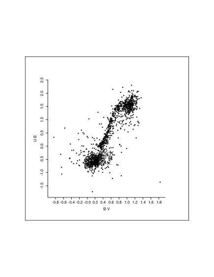
Figure 7: $(U-B)/(B-V)$ colour-colour diagram showing the $\chi^{2}$-selected white dwarf candidates within the area covered by the optical data.

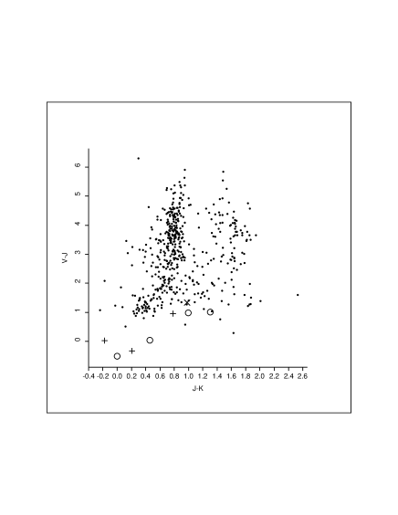
Figure 8: $(V-J)/(J-K)$ colour-colour diagram showing the $\chi^{2}$-selected white dwarf candidates within the area covered by the optical/infrared data.

The results obtained from the $\chi^{2}$-analysis of the optical/infrared data are as follow: a total of 21 candidates are selected with 18 being robust detections. Figure 8 shows the distribution of the candidates in the same colour-colour diagram as Figure 2. The locus of the white dwarves in this diagram is shifted redwards relative to that computed by P. Bergeron (2001). The candidates have estimated effective temperatures in the range 6000 to 14000K. The overlap between the sub-samples extracted from the five and seven passband comprises 18 objects. The remaining three objects were originally classified as quasar candidates. Another 17 objects selected as white dwarf candidates based on the optical only, are now classified as quasar candidates. These results show how difficult it is to distinguish between quasars and white dwarves, and how useful the infrared data can be for that purpose.

It is worth pointing out that none of the cool white dwarf candidates identified using the optical colours are confirmed when the infrared colours are included in the analysis. This may be due to inadequacies in the near-infrared part of the model spectra, which could also explain the shift of the locus of white dwarf candidates mentioned above. This point will be further investigated when more infrared spectra become available.

Table 2 lists the first 40 entries of the white dwarf candidate sample, comprising 100 objects. The format is the same as in Table 1, with the effective temperature for the best-fit model presented in column (11).

Table 2: First 40 entries of the CDF-S white dwarf candidate list.

4.2.2 Low Mass Stars and Brown Dwarfs

The low mass and brown dwarf spectral library was provided by Chabrier and Baraffe and consists of 105 theoretical spectra. They correspond to three sets of models which attempt to account for differences in the formation and settling of dust in the atmospheres (Chabrier et al., 2000). In this paper 53 of these models are used, corresponding to objects with masses $\leavevmode\nobreak\ \hbox to0.0pt{$<$\hss}{\lower 4.30554pt\hbox{$\sim$}}0.1M_{\odot}$ ($T_{\rm eff}\leavevmode\nobreak\ \hbox to0.0pt{$<$\hss}{\lower 4.30554pt\hbox{$\sim$}}2800$K), to select low-mass stars and/or brown dwarf candidates. These template spectra were compared to our broad-band SED and over the 0.25 square degree area covered in five passbands a total of 18 candidates were identified with $18\leavevmode\nobreak\ \hbox to0.0pt{$<$\hss}{\lower 4.30554pt\hbox{$\sim$}}I\leavevmode\nobreak\ \hbox to0.0pt{$<$\hss}{\lower 4.30554pt\hbox{$\sim$}}22$ (all fainter than $B\sim 24$), with 13 being robust detections. All of the candidates are matched to spectra with effective temperatures between 1700K and 2800K, corresponding to masses roughly between 0.05 and 0.1 M_⊙, close to the hydrogen-burning limit. Their position on a $(V-R)/(R-I)$ diagram is shown in Figure 9. The objects with $(R-I)>2.5$ seen on this figure that have not been selected as low mass or brown dwarf candidates were identified as M6V stars. Note that this class marks the transition between main sequence stars and low mass stars. Comparing the results of the $\chi^{2}$-analysis with those obtained selecting objects redder than $(R-I)>2.3$, roughly corresponding to the $(V-I)>3.5$ criterion adopted by Zaggia et al. (1999), one finds a significant contamination ($\sim$75%) by other types of objects.

Applying the $\chi^{2}$-test on the optical/infrared data one finds a total of 35 candidates out of which 14 are robust classifications. All five low-mass star candidates that have both optical and near-infrared data are confirmed when the $J$ and $K_{s}$ information is included in the analysis. Furthermore, 11 stars originally classified as M5V and M6V stars using the $UBVRI$ catalogues, are classified as low-mass stars when the infrared data are used. All candidates lie in the range $15.5\leavevmode\nobreak\ \hbox to0.0pt{$<$\hss}{\lower 4.30554pt\hbox{$\sim$}}K_{s}\leavevmode\nobreak\ \hbox to0.0pt{$<$\hss}{\lower 4.30554pt\hbox{$\sim$}}19.0$ and have estimated effective temperatures in the range between 1700K and 2800K. The candidates identified are shown in Figure 10. The figure shows two main concentrations of low mass star candidates. One at $(J-K_{s})\sim 0.8$ and $(I-J)\sim 1.5$, with 19 candidates, roughly corresponding to the transition between main sequence and very low mass stars. The other covers the region defined by $(J-K_{s})\leavevmode\nobreak\ \hbox to0.0pt{$>$\hss}{\lower 4.30554pt\hbox{$\sim$}}1.4$ and $(I-J)\leavevmode\nobreak\ \hbox to0.0pt{$>$\hss}{\lower 4.30554pt\hbox{$\sim$}}1.8$ (13 objects), consistent with the location of the L-dwarves (L3) as reported in the literature (e.g. Reid et al., 2001; Leggett et al., 2001; Schweitzer et al., 2001). In this optical/infrared colour diagram, as mentioned in the previous sections, one sees again a population of objects with colours which are not predicted by any model describing the spectral properties of point-sources. As discussed below, most of these objects are associated with unresolved galaxies which contaminate the point-source catalogue.

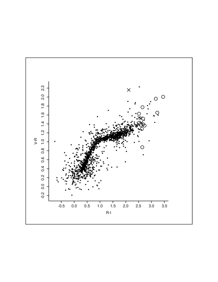
Figure 9: Optical colour-colour diagram showing the brown dwarf candidates selected from the $\chi^{2}$-technique.

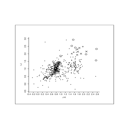
Figure 10: Optical/infrared colour-colour diagram showing the brown dwarf candidates selected using the $\chi^{2}$-technique.

Based on the results of the $\chi^{2}$-selection one finds a surface density of very low mass stars of about 72 candidates per square degree using optical colours. When the near-infrared data is added, this value increases by a factor of 3, yielding a surface density of 350 per square degree. These estimates for the surface density are a factor of 3 higher than the expected value of 116 low-mass stars per square degree with $T_{\rm eff}\leavevmode\nobreak\ \hbox to0.0pt{$<$\hss}{\lower 4.30554pt\hbox{$\sim$}}2800$K and brighter than $B=25$, predicted by models (e.g. Girardi et al., 2001).

The final list of individual low-mass star candidates in the CDF-S field is given in Table 3. The table format is the same as that of Table 2.

Table 3: List of low-mass star candidates in the CDF-S.

4.3 Very red objects

In the previous sections only objects detected in at least three passbands have been considered. There are, however, objects detected in one or two passbands, that may be of interest as well and for which neither the $\chi^{2}$-method nor colour-colour selection can be of use. Of particular interest are those detected in the red-most passbands available, e.g. $R$ and/or $I$ over 0.25 square degrees and $J$ and/or $K_{s}$ for 0.1 square degrees. While impossible to classify them having a single colour and, in some cases, just a lower limit, these very red objects are natural candidates for follow-up spectroscopy. However, they could also be associated with possible features in the colour catalogue production, as discussed in Section 5. Table 4 lists the identification, coordinates, colour (whenever available) and red-most magnitude of the objects detected in $R$ and $I$ (16 objects), in $I$ only (4 objects), in $J$ and $K_{s}$ (5 objects), and in $K_{s}$ only (4 objects).

Table 4: Very red objects detected in the red-most filters available.

Name	$\alpha(J2000)$	$\delta(J2000)$	$I$	$R-I$	Notes
EIS J033112.31-275640.1	03:31:12.31	-27:56:40.1	21.86	2.53
EIS J033119.40-274834.9	03:31:19.40	-27:48:34.9	21.73	3.75
EIS J033140.38-275942.9	03:31:40.38	-27:59:42.9	20.50	1.79	d
EIS J033141.54-273505.2	03:31:41.54	-27:35:05.2	21.64	2.94
EIS J033143.33-274707.3	03:31:43.33	-27:47:07.3	21.71	2.79
EIS J033155.88-280344.7	03:31:55.88	-28:03:44.7	21.22	2.58
EIS J033221.01-273659.1	03:32:21.01	-27:36:59.1	20.89	2.12	d
EIS J033226.53-273721.2	03:32:26.53	-27:37:21.2	21.60	3.38
EIS J033226.64-280248.9	03:32:26.64	-28:02:48.9	20.71	3.76
EIS J033249.39-273405.8	03:32:49.39	-27:34:05.8	21.45	3.75
EIS J033254.87-280224.1	03:32:54.87	-28:02:24.1	21.47	3.99
EIS J033257.33-280310.1	03:32:57.33	-28:03:10.1	22.00	2.68
EIS J033302.20-275914.4	03:33:02.20	-27:59:14.4	21.80	3.29
EIS J033317.64-274040.0	03:33:17.64	-27:40:40.0	21.94	1.58	d
EIS J033327.41-280253.5	03:33:27.41	-28:02:53.5	20.95	4.07
EIS J033342.70-274618.1	03:33:42.70	-27:46:18.1	21.87	1.91
EIS J033132.87-274111.4	03:31:32.87	-27:41:11.4	21.11	$>$4.9	d
EIS J033211.00-275904.7	03:32:11.00	-27:59:04.7	21.86	$>$4.1	d
EIS J033230.20-273337.6	03:32:30.20	-27:33:37.6	21.12	$>$4.8	d
EIS J033251.60-275917.5	03:32:51.60	-27:59:17.5	21.57	$>$4.4	d
Name	$\alpha(J2000)$	$\delta(J2000)$	$K_{s}$	$J-K_{s}$	Name
EIS J033229.58-274812.5	03:32:29.58	-27:48:12.5	19.86	2.24
EIS J033238.14-274750.1	03:32:38.14	-27:47:50.1	20.33	1.37
EIS J033241.92-274512.5	03:32:41.92	-27:45:12.5	20.32	1.29
EIS J033245.80-274211.4	03:32:45.80	-27:42:11.4	19.98	1.13	d
EIS J033304.21-275137.3	03:33:04.21	-27:51:37.3	19.25	1.00	d
EIS J033225.12-274219.7	03:32:25.12	-27:42:19.7	19.09	$>$4.3	d
EIS J033226.12-274327.0	03:32:26.12	-27:43:27.0	20.42	$>$3.0
EIS J033242.43-274236.7	03:32:42.43	-27:42:36.7	19.71	$>$3.7	d
EIS J033307.51-274435.6	03:33:07.51	-27:44:35.6	20.18	$>$3.2	d

Figure 11 shows the $(R-I)\times I$ colour-magnitude diagram for all point-sources within the area of 0.25 square degrees (left panel) and the $(J-K_{s})\times K_{s}$ diagram for the central area of the CDF-S covered by infrared data (right panel). The symbols are described in the figure caption. The extreme colour lower limits of the $R$- and $J$-dropouts shown in the figure make them likely to be brown dwarves (but see Section 5).

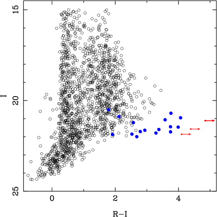
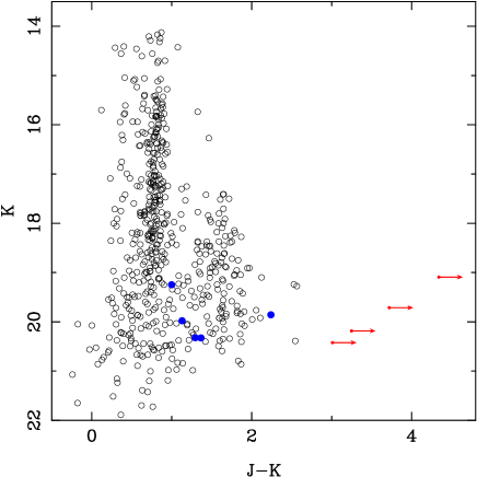
Figure 11: Colour - magnitude diagrams for the very red objects: $I$ versus $R-I$ (left panel) and $K_{s}$ versus $J-K_{s}$ (right panel). The filled circles show objects detected in two bands. Arrows indicate lower limits in the colour of objects detected only in the red-most passband.

4.4 Outliers

As discussed in Section 3.2 there are several reasons why one would like to search for outliers. From a pure technical point of view, objects with odd colours have to be identified and visually inspected as they may reveal problems in the construction of the colour catalogue, contamination by close neighbours, cosmic rays or other image artifacts. Alternatively, they may represent potentially interesting rare cases, either of known objects such as quasars at very high-redshifts or previously unknown populations. Therefore, classifying objects as outliers is an important step towards verifying the integrity of the colour catalogue and avoiding overlooking new discoveries.

Figure 12: Illustration of the selection of outliers applied on the five passband sub-sample for $m=2$. For definitions of d${}_{S_{1}}$ and d${}_{S_{2}}$ see Section 3.

As described in Section 3.2, outliers are identified in colour space based on their distances d${}_{S_{1}}$ and d${}_{S_{2}}$ from their nearest neighbour. An isolation criterion is then chosen, depending on the position of the objects on the d${}_{S_{1}}$ versus d${}_{S_{2}}$ diagram, as schematically shown in Figure 12. This criterion divides the d${}_{S_{1}}$ versus d${}_{S_{2}}$ space in two regions, a densely populated one towards low values of the parameters and a much less dense region, where outliers lie. The parameters describing the separation line are chosen by fine-tuning them to include the most obvious cases of isolated objects in different colour-colour projections, separately for $m=2$ and $m=3$. Note, however, that objects isolated in one of the colour-colour projections are not necessarily isolated in all of them.

Table 5: Number of objects identified as outliers for different samples.

Sub-sample	N	$m=2$	$m=3$
$UBVRI$	1164	19	26
$BVRI$	300	13	17
$UBVRIJK_{s}$	385	19	18
$BVRIJK_{s}$	119	13	19

The results from the outlier analysis are summarised in Table 5, which lists the sub-samples, the number of objects in them and the number of outliers for $m=2$ and $m=3$, respectively. Note that in general the number of outliers increases with $m$. From the table one finds that the fraction of outliers is small being typically $\sim$10% of the whole sample. For both $m=2$ and $m=3$, about 60% of the outliers are indeed poorly classified by the $\chi^{2}$-method, while 30% are robust candidates. These results indicate, as expected, that the outliers consist of a mix population including known rare objects, objects possibly not well described by the available spectral library, or undesirable features on the images or the derived catalogues. The total number of outliers is 64 (80) for the sub-samples analysed using $m=2$ ($m=3$), out of which about 60% deserve a closer investigation as presented in the next Section.

Figure 13 illustrates the location of outliers identified by applying the methodology described above to the five (seven) passband sub-sample. The figure shows two projections of the colour space, one for each of the sub-samples considered. The different symbols represent outliers selected using different values of $m$. Since nearly all of the outliers identified using $m=2$ are also identified when $m=3$ is used, in these plots only the additional objects identified with $m=3$ are represented by a different symbol. While a single projection is not sufficient to determine whether an object is truly an outlier in the multi-dimensional colour space, most objects far from the main concentration of points are successfully identified. In particular, in the left panel one finds the object with very particular colours, mentioned in section 4.1, originally classified as a quasar. This case as well as others will be discussed in the next Section.

Generally speaking, among the 30% of outliers which are also robust $\chi^{2}$ classifications about half are identified as quasar candidates and half are identified as galactic object candidates from the $\chi^{2}$-technique. In both cases, the candidates found to be outliers are associated with sparse populations with nearly all quasars having $z\leavevmode\nobreak\ \hbox to0.0pt{$>$\hss}{\lower 4.30554pt\hbox{$\sim$}}3$ and most of the stars being early spectral types (O-A) which are rare, especially at high-galactic latitudes. These results apply equally well to all the sub-samples and isolation criteria adopted.

Note that the selection of the $m-th$ neighbour as well as the separation line must be empirically determined. Even thought there is a correspondence between the outlier selection and the values of the $\chi^{2}$, the exact relation is not easy to establish.

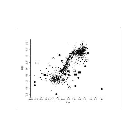
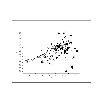
Figure 13: $(U-B)/(B-V)$ (left panel) and $(B-V)/(V-K_{s})$ (right panel) showing objects classified as outliers by the criteria given in Section 3 adopting $m=2$ (circles) and $m=3$ (rectangles). Open (filled) symbols denote objects with good (poor) classifications.

5 Evaluation of Classification Results

In previous sections the results of the $\chi^{2}$ classification were tentatively assessed by comparing these classifications with those that would be obtained from selecting regions in two-colour diagrams. In this section this evaluation is complemented by an investigation of the nature of the outliers and extreme red objects detected in two or only one band, in several cases resorting to a visual inspection of the images and a careful examination of the photometric measurements obtained for these objects. The motivation is to find possible effects that may impact the $\chi^{2}$ fitting and lead to a poor classification. The primary goal is to investigate whether these cases are of interest or are, instead, associated with particularities of the images and/or derived source catalogues for which, perhaps, additional refinements in the selection criterion can be devised. The measured SED of the poorly classified objects are also compared to a set of galaxy models to evaluate the possible contamination of the point-source catalogue by unresolved galaxies. The information stemming from the discussion below is incorporated as notes to the Tables 1, 2, 3, and 4. In these notes “o” denotes outliers, “d” objects that should be discarded from further consideration, and “g” objects which are better matched by galaxy spectra.

5.1 Nature of Outliers

Out of a total of 81 outliers, representing less than 5% of the total sample of point-sources, image cutouts were produced for all 57 objects having poor classification based on the $\chi^{2}$-analysis. From the visual inspection of their images the following conclusions can be drawn. About 44% of the cases (25 objects) are found to be significant SExtractor detections, point-like sources and isolated. This set of objects consists of a mixed population which includes predominantly and high-redshift quasars ($2.1<z<3.94$) candidates. Among them there are two interesting cases, both poorly classified as quasars, one of which has already been mentioned in Section 4.1 (Figure 1). Close examination of their photometry shows that both objects have comparable magnitudes in all passbands except in $B$ in which they are more than one magnitude fainter. Inspection of the original images show no reason to suspect problems in the magnitude estimates. The only possible explanation for the odd colours is that these objects may be variable. This seems to be a reasonable explanation considering that images taken in all passbands except $B$ were obtained a few days apart, while the $B$-images were taken nine months earlier. This result points out the importance of including temporal information, whenever possible, in the type of analysis presented here.

About 25% of poorly classified outliers are located near other objects leading to problems of contamination, de-blending and erroneous associations and should be discarded. The remaining 30% of the cases have been identified with features of the source extraction algorithm and with the production of colour catalogues, which are now being addressed.

In summary, about 25% of the outliers are robust classifications. Another 25% are isolated objects with no apparent problems in their photometric measurements, indicating that their poor classification may be due to inadequacies in the spectra library. These objects are thus prime targets for spectroscopic observations. These cases as well as outliers found to be potentially problematic are indicated in the tables of different classification types presented in previous sections. Taken the above numbers at face value one can conclude that only for about 2% of the objects in the original point-source colour catalogue should be discarded because of problems, most of which unavoidable in nature being caused by the presence of nearby objects affecting their photometric measurements.

5.2 Very Red Objects

In addition to the outliers one should also carefully examine extreme cases such as those presented in Section 4.3. From the total of 29 objects listed in Table 4, 17 showed no problems when visually inspected. Out of the remaining 12, seven are close (less than 4 arcsec) to brighter objects or located on the outer parts of a galaxy, and were not properly de-blended. Included are two $K$-only objects listed in Table 4. Another related case is one object found close to one of the masks automatically placed around a very bright star. As before, the photometric measurements are not reliable. Two additional problems were recognized. One is the break-up of a galaxy image by the source extraction algorithm (1 case) and the detection of residual cosmic rays in regions poorly sampled by the dithered images (2 cases, both $I$-only detections). Finally, one $JK_{s}$-only object, while visible in the $I$-band image, was not detected.

5.3 Contamination by Galaxies

While the bright catalogue considered here should, in principle, contain only point sources, objects having poor classification (see Section 3) according to the $\chi^{2}$-method have also been compared to galaxy templates. Overall there are 216 and 221 objects with poor classification in the five and seven passband catalogues, respectively. From their comparison with galaxy spectra one finds that 25 - 35% have an improved fit, with 51 and 71 objects being classified as galaxies, respectively. The objects classified as galaxies have mix morphological classifications and cover a broad redshift range. Based on these numbers one estimates that a lower-limit for the contamination of the five and seven passband point-source catalogues by unresolved galaxies is of the order of 5 - 10%.

6 Discussion

The methodology described in this paper has been developed to analyse in an objective and automatic way colour catalogues being routinely produced by the EIS pipeline in order to: assign objects to different classes of astronomical sources; allow for new discoveries; and understand the limitations of the data and the procedures adopted in the derivation of source catalogues and their colours from the association of data taken in different passbands. The ultimate goal is to define procedures to efficiently extract from imaging survey data well-defined samples, with minimal contamination, for spectroscopic follow-ups.

As a first step in this direction the method of $\chi^{2}$ fitting template spectra to the measured broad-band photometry, currently being used for estimating galaxy/quasar photometric redshifts, has been employed, extending it to include different types of galactic objects. The method is intended to replace standard classification schemes based on the analysis of one or more two-colour diagrams which becomes unmanageable for large sets of multi-band data. As currently implemented the classification scheme only considers the spectral properties of the objects, neglecting other important information as the apparent magnitude of the objects and the expected density of objects of different types (see below). The results obtained from the automatic classification are not only consistent with those that would have been obtained from traditional methods based on two-colour diagrams but also consistent with model predictions, while minimising contamination by objects of other types. A point worth noting is that a significant number of poor classifications stem from the fact that the passbands used in the present analysis not always provide independent information and the statistical analysis leads to artificially low significances of the resulting classifications. In order to deal with this problem other techniques which take into account the proper dimensionality of the colour space for a specific class of objects (e.g. PCA) should also be considered. Finally, it is worth emphasising that the classifications are as good as the available spectral library. The library currently being used has been assembled from publicly available models and data and a number of classes are under-represented. Improvements in the classification method will depend on the continuous upgrade of the available spectral library. Currently, the library is being upgrade to include infrared spectra of white dwarves and low-mass stars kindly provided by S. Leggett. Adding spectra for different type of objects from other ongoing spectroscopic surveys such as the SDSS will also be of great value in improving the current library.

In order to detect potential problems and not to overlook possible new discoveries the $\chi^{2}$-method has been complemented by a procedure of identifying outliers using as dissimilarity measures Euclidean distances in the multi-dimensional colour space and adopting a nearest-neighbour isolation criterion. Despite its simplicity the criterion adopted identified rare population of objects, objects with odd colours which could be traced either to real physical effects such as variability or to problems with their measured colour, demonstrating its usefulness in greatly reducing the number of cases, about 5% of the entire sample, that require a more detailed inspection. This number could be reduced even more by a further screening of the sample. As alluded to in the previous section, information about variability, if available, is of great use as it is a criterion based on angular separation and magnitude differences between a source and its nearest neighbour or to the mask automatically placed around very bright stars. This together with SExtractor de-blending flag and distance to masks placed around very bright stars should be used to discard objects which are likely to have the photometry affected by light contamination, the most common problem identified.

Overall, the present analysis suggests that derived catalogues are mostly free of problems. Visual inspection of several odd colour or extremely red objects has revealed that the most frequent problems are associated to the limitations of the de-blending algorithm; contamination by close neighbours; and, in some cases, residual cosmic rays located in poorly sampled regions of the image mosaic, with insufficient number of stacked images for a proper sigma-clipping.

In a follow-up paper the classification based on the spectral properties, as presented here, will be complemented with other statistics which further characterize the different populations of extragalactic/galactic objects using mock catalogues created from Monte Carlo simulations. This is particular important in the analysis of point-sources for which the stellar population makes an important contribution which varies according to the position of the sky observed. To account for this as well as reddening effects and the different filter sets used by the various surveys a population synthesis model has been combined with galactic structure models to simulate different observations.

7 Summary

This paper describes the methodology developed to analyse multi-wavelength data from ongoing public surveys to objectively and automatically classify extracted objects based on their colours. The method is expected to yield samples with better completeness and less contamination, than previous analysis based on two-colour diagrams. Moreover, the analysis can be carried out automatically and thus better cope with the rapidly increasing data volume from imaging surveys and more efficiently producing improved samples (higher yield) to feed large-aperture telescopes. The method has been applied to a catalogue of point-sources extracted from the optical/infrared images taken of the CDF-S field by the EIS project. The CDF-S field is of particular interest in this context considering the number of spectroscopic and photometric programs either ongoing or planned for the near future. These data will be invaluable to directly assess the results of the present analysis which may lead to refinements in the classification method adopted. The paper also provides a rough estimate of the by-products that should be expected at the end of the ongoing DPS.

The data used consists of $UBVRI$ images taken with a wide-field imager covering an area of 0.25 square degree, complemented by a mosaic of infrared $JK_{s}$ images covering 0.1 square degrees. Combining these data one finds a total of 234 quasar candidates with estimated photometric redshifts up to $z\sim 5$, among which 16 have $z\leavevmode\nobreak\ \hbox to0.0pt{$>$\hss}{\lower 4.30554pt\hbox{$\sim$}}3.5$. In addition, 51 low-mass star/brown dwarf candidates and 100 white dwarf candidates were identified. Tables listing the classified objects are presented together with the properties inferred by the classification method. If the classifications presented here are confirmed, samples comprising over 200 high-redshift quasars ($z>$3.5), and over 1000 white dwarves, $\sim$100 cooler than 4000K, will become available at the end of the survey, expected to cover 3 square degrees.

It is worth emphasising the contribution of the near-infrared data. It increases the accuracy of the determination of the photometric redshifts as well as the number of quasar candidates in the redshift interval $2.5\leavevmode\nobreak\ \hbox to0.0pt{$<$\hss}{\lower 4.30554pt\hbox{$\sim$}}z\leavevmode\nobreak\ \hbox to0.0pt{$<$\hss}{\lower 4.30554pt\hbox{$\sim$}}3.5$. Infrared photometry is also essential for tracking very low-mass stars and brown dwarves. If only optical data are considered, one should expect the DPS to provide $\sim$200 low-mass stars, including only $\sim$20 L-dwarves over the 3 square degree area. Since the surface density of L-dwarves increases to 120 per square degree when infrared data is considered, the number of L-dwarves would be much larger if the infrared observations were extended. As it currently stands the infrared observations cover an area of 0.2 square degrees within which one expects $\sim 25$ L-dwarves.

The results presented here will be used in a forthcoming paper to produce a pruned stellar catalogue (Groenewegen et al., 2001). The same techniques will also be applied to analyse the faint source catalogue of the CDF-S which should also yield interesting results and more insight regarding the source catalogues.

Finally, one should keep in mind that, unless follow-up spectroscopic studies of the current samples are carried out, the numbers and target list will remain tentative.