Patterns in the weak shear 3-point correlation function

We explore the scale and angular dependence of the cosmic shear three-point correlation function. The shear field is found to have a much more complex three-point function than the convergence field, but it also exhibits specific motifs which draw signatures of gravitational lensing. Exact shear patterns are inferred analytically for some geometrical shear triplets configurations, when simple interpretations can be derived. A more complete description of their geometrical properties has then been carried out from ray-tracing numerical simulations and simple models. These patterns reveal typical features that can be utilized for non-gaussian signal detection in cosmic shear surveys. We test the robustness of these properties against complex noise statistics and non-trivial survey topologies. From these conclusive checks, we predict that the VIRMOS-DESCART survey should allow a detection of a non-gaussian signal with a comfortable significance for a low matter density Universe.

1 Introduction

The detections of cosmic shear signal (van Waerbeke et al. 2000, Bacon et al. 2000, Wittman et al. 2000, Kaiser et al. 2000, Maoli et al 2001) opened the analysis of large-scale mass distribution in the Universe to weak lensing surveys. As the surveys sizes progressively increase, the noise and systematics are reduced to reasonable levels, which permits to constrain cosmological parameters from the amplitude and the shape of the shear two-point correlation function (Maoli et al. 2001, van Waerbeke et al. 2001b). However, although it is weakly sensitive to the cosmological constant $\Omega_{\Lambda}$ (Bernardeau, van Waerbeke & Mellier 1997), the two-point function is a degenerate combination of the matter density $\Omega_{{\rm m}}$ of the Universe and the amplitude of the power spectrum $\sigma_{8}$ (Villumsen 1996, Jain & Seljak 1997).
This degeneracy can be broken from the angular dependence of the cosmic shear amplitude (Jain & Seljak 1997), but it relies on the prior knowledge of the shape of the mass power spectrum. An alternative is to directly probe weak shear maps, which contain non-gaussian features that can be used to derive $\Omega_{{\rm m}}$ with the only assumption that initial conditions were gaussian (Bernardeau, van Waerbeke, Mellier 1997, van Waerbeke, Bernardeau, Mellier 1999) - this later assumption being eventually testable in the data set itself .
So far, all the theoretical predictions regarding non-gaussian features are based on a critical reconstruction process of either a convergence map (filtered for instance with a top-hat window function) or an aperture mass map (Kaiser et al. 1994, Schneider 1996, Schneider et al. 1998, Bernardeau & Valageas 2000). Unfortunately, the panoramic reconstruction of mass maps from real data turned out to be considerably more difficult than expected. The masking process discussed by van Waerbeke et al. 2000 produces patchy surveys with a non-trivial topology and inhomogeneous noise. The resulting mass maps have poorly understood statistical properties which is practically difficult to handle with confidence. We therefore explore another option which uses direct signatures of gaussian effects in shear map patterns.

Shear pattern study is a priory more difficult because the third order moment of the local shear vanishes for obvious symmetry reasons. It is therefore necessary to seek for peculiar configurations (or geometries) of shear triplets for which a significant signal is expected. This is the aim of this paper. In the next section, we present the exact analytical results obtained for specific geometries, their interpretation and the results obtained from ray-tracing simulations which exhibit the complete three-point function patterns. The detection of these features in these simulations is presented in section 3. These results suggest a detection strategy in cosmic shear surveys which is put forward and tested with mock catalogs in section 4. We checked carefully that the masks do not compromise the possibility of detecting the effect. Finally, we estimate the expected error level of such measurements in the available data sets.

2 Theoretical insights

2.1 The local shear statistical properties

In the following we assume the shear signal is entirely due to cosmic shear effects, and there is no so-called $B$-mode produced by lens-lens coupling, clustering or any other contamination. Later in the paper (in Section 4) we study the impact of residual systematics. This hypothesis naturally leads to derive the shear field ${\@vec{\gamma}}$ from a potential field which can be written, in Fourier space,

$${\@vec{\gamma}}({\@vec{x}})=\int{\rm d}^{2}{\@vec{l}}\,\kappa_{{\@vec{l}}}\,\exp({\rm i}{\@vec{l}}.{\@vec{x}})\,{\@vec{u}}(\theta_{{\@vec{l}}})$$ (1)

with

$${\@vec{u}}(\theta_{{\@vec{l}}})=\left(\begin{array}[]{c}\cos(2\theta_{{\@vec{l}}})\\ \sin(2\theta_{{\@vec{l}}})\end{array}\right),$$ (2)

where $\kappa_{{\@vec{l}}}$ is the Fourier transform of the local convergence map, the components of ${\@vec{l}}$ being $l\cos(\theta_{{\@vec{l}}})$ and $l\sin(\theta_{{\@vec{l}}})$. We also assume the validity of the small angle approximation, making the spherical harmonic decomposition unnecessary (Stebbins 1996).

The statistical properties of the variable $\kappa_{{\@vec{l}}}$ can be inferred from those of the projected density contrast. These derivations have been studied in details in the many papers mentioned in the introduction. Using the small angle approximation (Limber 1954, applied here in Fourier space, Kaiser 1992, 1998, Bernardeau 1995), they give the expression of the convergence power spectrum $P_{\kappa}(l)$, defined as,

$$\langle\kappa_{{\@vec{l}}}\kappa_{{\@vec{l}}^{\prime}}\rangle=\delta_{\rm Dirac}({\@vec{l}}+{\@vec{l}}^{\prime})\,P_{\kappa}(l)$$ (3)

as an integral over the line-of-sight of the 3D matter density contrast power spectrum $P_{\delta}(k)$,

$$P_{\kappa}(l)=\int_{0}^{\chi_{{\rm CMB}}}{{\rm d}\chi\over{\cal{D}}^{2}}\,w^{2}(\chi)\,P_{\delta}\left(k\over{\cal{D}}\right)$$ (4)

where $w(\chi)$ is the lensing efficiency function ($\chi$ is the radial distance, ${\cal{D}}$ is the comoving angular distance). It depends on the cosmological parameters and on the source redshift distribution function, $n(z_{s})$:

$$w(\chi)={3\over 2}\Omega_{{\rm m}}\int{\rm d}z_{s}\,n(z_{s}){{\cal{D}}(\chi_{s}-\chi)\,{\cal{D}}(\chi)\over a\,{\cal{D}}(\chi_{s})}$$ (5)

where $\chi_{s}$ is the radial distance to the source plane and when the distances are expressed in units of $c/H_{0}$. The phenomenological properties of the convergence field, or similarly the shear field, will be determined by both the shape of the efficiency function and the properties of the cosmic density field.

Likewise, the convergence three-point function can be derived from the cosmic matter three-point function. The small angle approximation can indeed be used again at this level (Bernardeau 1995, Bernardeau et al. 1997), leading to the expression of the ${\@vec{l}}$-space three point function

$$\langle\kappa_{{\@vec{l}}_{1}}\kappa_{{\@vec{l}}_{2}}\kappa_{{\@vec{l}}_{3}}\rangle=\delta_{\rm Dirac}({\@vec{l}}_{1}+{\@vec{l}}_{2}+{\@vec{l}}_{3})\,B_{\kappa}({\@vec{l}}_{1},{\@vec{l}}_{2},{\@vec{l}}_{3})$$ (6)

with

$$B_{\kappa}({\@vec{l}}_{1},{\@vec{l}}_{2},{\@vec{l}}_{3})=\int_{0}^{\chi_{{\rm CMB}}}{{\rm d}\chi\over{\cal{D}}^{2}}\,w^{3}(\chi)\,B_{\delta}\left({{\@vec{l}}_{1}\over{\cal{D}}},{{\@vec{l}}_{2}\over{\cal{D}}},{{\@vec{l}}_{3}\over{\cal{D}}}\right)$$ (7)

where $B_{\delta}({\@vec{k}}_{1},{\@vec{k}}_{2},{\@vec{k}}_{3})$ is the 3D matter density contrast bispectrum:

$$\langle\delta_{{\@vec{k}}_{1}}\delta_{{\@vec{k}}_{2}}\delta_{{\@vec{k}}_{3}}\rangle=\delta_{\rm Dirac}({\@vec{k}}1+{\@vec{k}}_{2}+{\@vec{k}}_{3})\,B_{\delta}({\@vec{k}}_{1},{\@vec{k}}_{2},{\@vec{k}}_{3}).$$ (8)

The bispectrum $B_{\delta}$ is usually parametrized as follows

$$B_{\delta}({\@vec{k}}_{1},{\@vec{k}}_{2},{\@vec{k}}_{3})=Q({\@vec{k}}_{1},{\@vec{k}}_{2})P_{\delta}(k_{1})P_{\delta}(k_{2})+{\rm sym.}\ ,$$ (9)

where $Q$ is an homogeneous function of the wave vectors ${\@vec{k}}_{1}$ and ${\@vec{k}}_{2}$. For instance, in the quasi-linear regime it is given by,

$$Q({\@vec{k}}_{1},{\@vec{k}}_{2})={10\over 7}+{{\@vec{k}}_{1}.{\@vec{k}}_{2}\over k_{1}^{2}}+{{\@vec{k}}_{1}.{\@vec{k}}_{2}\over k_{2}^{2}}+{4\over 7}{({\@vec{k}}_{1}.{\@vec{k}}_{2})^{2}\over k_{1}^{2}\,k_{2}^{2}}\ ,$$ (10)

whereas in the nonlinear regime $Q$ is often assumed to be a pure number (that depends however on the cosmological models). Several phenomenological models have been proposed to describe the behavior of the three-point matter correlation function, from the quasi-linear regime to the nonlinear regime (the so-called EPT, Colombi et al. 1997 or its extensions with the HEPT, Scoccimarro & Frieman 1999). In particular Scoccimarro & Couchman (2001) have shown that the matter three-point function could be described by,

$$Q({\@vec{k}}_{1},{\@vec{k}}_{2}) = a(k_{1},k_{2})+b(k_{1},k_{2})\left({{\@vec{k}}_{1}.{\@vec{k}}_{2}\over k_{1}^{2}}+{{\@vec{k}}_{1}.{\@vec{k}}_{2}\over k_{2}^{2}}\right)+$$ (11)

$$+c(k_{1},k_{2}){({\@vec{k}}_{1}.{\@vec{k}}_{2})^{2}\over k_{1}^{2}\,k_{2}^{2}},$$

where $a$, $b$ and $c$ depend on scale in a known way.

The properties of the 3D matter three-point function actually extend to the three-point correlation function of the convergence field; e.g. one expects to have

$$B_{\kappa}({\@vec{l}}_{1},{\@vec{l}}_{2},{\@vec{l}}_{3})=Q_{\kappa}({\@vec{l}}_{1},{\@vec{l}}_{2})P_{\kappa}(l_{1})P_{\kappa}(l_{2})+{\rm sym.}.$$ (12)

To a large extent the functional dependence of the three-point function coefficient $Q_{\kappa}$ is left unchanged (Tóth, Hollósi & Szalay 1989, Bernardeau 1995) although its amplitude is affected by projection effects. This has been investigated in detail at the level of the convergence reduced skewness, which is proportional to the angular averages of $Q_{\kappa}({\@vec{k}}_{1},{\@vec{k}}_{2})$. Interestingly the reduced skewness, defined as

$$s_{3}={\langle\kappa^{3}\rangle\over\langle\kappa^{2}\rangle^{2}},$$ (13)

depends on the efficiency function amplitude, and therefore on the cosmological parameter, $\Omega_{{\rm m}}$, but is less sensitive to the cosmological constant value or the vacuum equation of state (Benabed & Bernardeau 2001). For sources at redshift about unity, calculations give (Bernardeau et al. 1997, Hui 1999, van Waerbeke et al. 2001a),

$$s_{3}\sim{\Omega_{{\rm m}}^{-0.8}},$$ (14)

irrespective of the amplitude of the matter fluctuation . This result actually extents to the amplitude of the convergence three-point function so that one expects to have,

$$Q_{\kappa}\sim{\Omega_{{\rm m}}^{-0.8}},$$ (15)

also. In the following the inter-relation between $Q$ and $s_{3}$ will be investigated in more details. But it is already obvious that a measurement of $Q$ would be useful to constrain the matter density parameter of the Universe.

2.2 The shear three-point function

The general expression for the shear three-point function can be inferred from the ${\@vec{l}}$-space three point function of the convergence field. However, because ${\@vec{\gamma}}$ is a 2 component pseudo-vector field there are many possible ways to combine shear triplets. The properties of shear patterns produced by these triplets may be complex. In order to interpret them in a cosmological context it is preferrable to focus first on few of them that can be easily investigated with analytical calculations. This is the case for $\left\langle\left({\@vec{\gamma}}({\@vec{x}}_{1}).{\@vec{\gamma}}({\@vec{x}}_{2})\right){\@vec{\gamma}}({\@vec{x}}^{\prime})\right\rangle$ for a fixed ${\@vec{x}}_{2}-{\@vec{x}}_{1}$ separation which is a vectorial quantity. This function displays a specific pattern which can be viewed as a 2D vector field.

2.2.1 Computation of $\langle\gamma^{2}({\@vec{x}}){\@vec{\gamma}}({\@vec{x}}^{\prime})\rangle$

Figure 1: Shear patterns in the vicinity of one of the pair point either ${\@vec{x}}_{1}$ or ${\@vec{x}}_{2}$ (positioned at the center of the plot) for $n=-1.5$, $n=-1.$ and $n=-0.5$ (from left to right) as a function of ${\@vec{x}}^{\prime}$. It illustrates the results of Eq. (46). Coordinates are arbitrary.

Let start with a simple configuration, when ${\@vec{x}}_{1}$ and ${\@vec{x}}_{2}$ are pointing in the same location ${\@vec{x}}$, for which case we have ${\@vec{\gamma}}({\@vec{x}}_{1}).{\@vec{\gamma}}({\@vec{x}}_{2})=\gamma^{2}({\@vec{x}})$. In this case the results make sense only when the filtering effects are taken into account. Otherwise the result is dominated by the shear behavior at arbitrarily small scale and depends on the detailed behavior of the power spectrum and bi-spectrum in the limit $k\to\infty$; in a regime that might be totally irrelevant for the observations. The shear field is averaged within a smoothing window, but in order to keep a simple notation, we still denote ${\@vec{\gamma}}({\@vec{x}})$ the smoothed shear vector at the window location ${\@vec{x}}$. For a top-hat window function of radius $\theta_{0}$, the three-points function can be written as,

$$\langle\gamma^{2}({\@vec{x}}){\@vec{\gamma}}({\@vec{x}}^{\prime})\rangle =$$ (16)

$$\int{\rm d}^{2}{\@vec{l}}\,{\rm d}^{2}{\@vec{l}}^{\prime}\,W(l\,\theta_{0})\,W(|{\@vec{l}}+{\@vec{l}}^{\prime}|\theta_{0})\,W(l^{\prime}\,\theta_{0})\,P_{\kappa}(l)\,P_{\kappa}(l^{\prime})\times$$

$$\,Q_{\kappa}({\@vec{l}},{\@vec{l}}^{\prime})\left[2\cos(2\theta_{{\@vec{l}}+{\@vec{l}}^{\prime}}-2\theta_{{\@vec{l}}^{\prime}})\,e^{{\rm i}{\@vec{l}}^{\prime}.({\@vec{x}}^{\prime}-{\@vec{x}})}\,{\@vec{u}}(\theta_{{\@vec{l}}^{\prime}})+\right.$$

$$\left.\cos(2\theta_{{\@vec{l}}}-2\theta_{{\@vec{l}}^{\prime}})\,e^{{\rm i}({\@vec{l}}+{\@vec{l}}^{\prime}).({\@vec{x}}^{\prime}-{\@vec{x}})}\,{\@vec{u}}(\theta_{{\@vec{l}}^{\prime}+{\@vec{l}}})\right]$$

where $W$ is the ${\@vec{l}}$-space top-hat window function,

$$W(x)={J_{1}(x)\over x},$$ (17)

where $J_{1}(x)$ is the first Bessel function of the first kind.

The computation of expression (16) is still complicated in general, but it simplifies in the large separation limit, $\theta_{0}\ll|{\@vec{x}}-{\@vec{x}}^{\prime}|$. In this case it is possible to express the result in terms of the square root of the variance of the filtered convergence $\sigma_{\kappa}$ and the convergence-shear correlation function $\xi_{\kappa\,\gamma}$.

In the large separation limit, in the first term of Eq. (16), the values of $l^{\prime}$ that will most contribute are of the order of $1/|{\@vec{x}}-{\@vec{x}}^{\prime}|$ whereas that of $l$ will be of the order of $1/\theta_{0}$; in the second term the integration in $l$ and $l^{\prime}$ factorize out (in this configuration $W(|{\@vec{l}}^{\prime}+{\@vec{l}}|)$ does not play any role) and both $l$ and $l^{\prime}$ are of the order of $1/\theta_{0}$. As a consequence the first term of (16) is of the order of $\sigma^{2}_{\kappa}\,\xi_{\kappa\,\gamma}$ whereas the second is of the order of $\xi^{2}_{\kappa\,\gamma}$ and is thus smaller. Furthermore, as in the first term $l^{\prime}\ll l$, it is possible to expand all quantities in $l^{\prime}/l$,

$$\cos(2\theta_{{\@vec{l}}+{\@vec{l}}^{\prime}}-2\theta_{{\@vec{l}}^{\prime}}) \approx 1-{l^{\prime 2}\over 2\,l^{2}}\sin^{2}(\theta_{{\@vec{l}}}-\theta_{{\@vec{l}}^{\prime}})+\dots$$ (18)

$$W(|{\@vec{l}}+{\@vec{l}}^{\prime}|\theta_{0}) \approx W(l\theta_{0})+l\theta_{0}\,W^{\prime}(l\theta_{0}){{\@vec{l}}.{\@vec{l}}^{\prime}\over l^{2}}+\dots$$ (19)

Once a shape for $Q_{\kappa}$ is given, computing the integral of the angle of ${\@vec{l}}$ is straightforward. In general, following the prescription of Scoccimarro & Couchman, Eq. (11), one can write

$$Q_{\kappa}({\@vec{l}},{\@vec{l}}^{\prime})=a(l,l^{\prime})+b(l,l^{\prime})\left({{\@vec{l}}.{\@vec{l}}^{\prime}\over l^{2}}+{{\@vec{l}}.{\@vec{l}}^{\prime}\over l^{\prime 2}}\right)+c(l,l^{\prime}){({\@vec{l}}.{\@vec{l}}^{\prime})^{2}\over l^{\prime 2}\,l^{2}}$$ (20)

from which one gets,

$$\langle\gamma^{2}({\@vec{x}}){\@vec{\gamma}}({\@vec{x}}^{\prime})\rangle = 2\pi\,\int l{\rm d}l\,{\rm d}^{2}{\@vec{l}}^{\prime}\,P_{\kappa}(l)\,P_{\kappa}(l^{\prime})\,e^{{\rm i}{\@vec{l}}^{\prime}.({\@vec{x}}^{\prime}-{\@vec{x}})}\times$$ (21)

$$\left\{W^{2}(l\,\theta_{0})\,W(l^{\prime}\,\theta_{0})\left[a(l,l^{\prime})+{c(l,l^{\prime})\over 2}\right]\right.+$$

$$\left.{l\theta_{0}\over 2}W(l\theta_{0})W^{\prime}(l\theta_{0})W(l^{\prime}\,\theta_{0})b(l,l^{\prime})\right\}\,{\@vec{u}}(\theta_{{\@vec{l}}^{\prime}}).$$

When $a(l,l^{\prime})$, $b(l,l^{\prime})$ and $c(l,l^{\prime})$ are pure numbers as it is the case for the quasi-linear regime, the integrals in $l$ and $l^{\prime}$ factorize and lead to an expression of the form,

$$\langle\gamma^{2}({\@vec{x}}){\@vec{\gamma}}({\@vec{x}}^{\prime})\rangle = c_{2\,1}\sigma^{2}_{\kappa}\times$$ (22)

$$\int{\rm d}^{2}{\@vec{l}}^{\prime}P_{\kappa}(l^{\prime})W(l^{\prime}\theta_{0})\,e^{{\rm i}{\@vec{l}}^{\prime}.({\@vec{x}}^{\prime}-{\@vec{x}})}\,{\@vec{u}}(\theta_{{\@vec{l}}^{\prime}})$$

where $c_{2\,1}$ is a pure number. It can actually be noted that $c_{2\,1}$ identifies with the coefficient appearing in the expression of the reduce joint cumulant,

$$\langle\kappa^{2}({\@vec{x}})\kappa({\@vec{x}}^{\prime})\rangle=c_{2\,1}\,\sigma^{2}_{\kappa}\,\langle\kappa({\@vec{x}})\kappa({\@vec{x}}^{\prime})\rangle$$ (23)

in the large separation limit (Bernardeau 1996). It has actually been already computed in Bernardeau et al. (1997) in the quasi-linear regime. It scales like $\Omega_{\rm m}^{-0.8}$ and it is mainly independent of the spectrum index.

The last integral in (22) is equal to the convergence-shear correlation function,

$${\@vec{\xi}}_{\kappa\,\gamma}({\@vec{x}}^{\prime})\equiv\int{\rm d}^{2}{\@vec{l}}^{\prime}P_{\kappa}(l^{\prime})W(l^{\prime}\theta_{0})\,e^{{\rm i}{\@vec{l}}^{\prime}.{\@vec{x}}^{\prime}}\,{\@vec{u}}(\theta_{{\@vec{l}}^{\prime}})\ ,$$ (24)

and can be computed by noticing that,

$$\int{\rm d}^{2}{\@vec{l}}^{\prime}P_{\kappa}(l^{\prime})W(l^{\prime}\theta_{0})\,e^{{\rm i}{\@vec{l}}^{\prime}.({\@vec{x}}^{\prime}-{\@vec{x}})}\,{\@vec{u}}(\theta_{{\@vec{l}}^{\prime}}) =$$ (27)

$$-\left(\begin{array}[]{c}\partial_{x^{\prime}}^{2}-\partial_{y^{\prime}}^{2}\\ 2\partial_{x^{\prime}}\partial_{y^{\prime}}\end{array}\right)\int{{\rm d}^{2}{\@vec{l}}^{\prime}\over l^{\prime 2}}P_{\kappa}(l^{\prime})W(l^{\prime}\theta_{0})\,e^{{\rm i}{\@vec{l}}^{\prime}.({\@vec{x}}^{\prime}-{\@vec{x}})}.$$

So, if one defines $\xi_{\phi}$ as the potential two-point correlation function,

$$\xi_{\phi}(x) = \int{{\rm d}^{2}{\@vec{l}}^{\prime}\over l^{\prime 2}}P_{\kappa}(l^{\prime})W(l^{\prime}\theta_{0})\,e^{{\rm i}{\@vec{l}}^{\prime}.{\@vec{x}}}$$ (28)

$$= 2\pi\int{{\rm d}l^{\prime}\over l^{\prime}}P_{\kappa}(l^{\prime})W(l^{\prime}\theta_{0})\,J_{0}(l^{\prime}\,x),$$

we get,

$$\int{\rm d}^{2}{\@vec{l}}^{\prime}P_{\kappa}(l^{\prime})W(l^{\prime}\theta_{0})\,e^{{\rm i}{\@vec{l}}^{\prime}.{\@vec{x}}^{\prime}}\,{\@vec{u}}(\theta_{{\@vec{l}}^{\prime}}) =$$ (31)

$$-\left(\begin{array}[]{c}x^{\prime 2}-y^{\prime 2}\\ 2\,x^{\prime}\,y^{\prime}\end{array}\right)\left[{1\over|{\@vec{x}}^{\prime}|^{2}}\xi^{\prime\prime}_{\phi}(|{\@vec{x}}^{\prime}|)-{1\over|{\@vec{x}}^{\prime}|^{3}}\xi^{\prime}_{\phi}(|{\@vec{x}}^{\prime}|)\right].$$

Therefore, in the case of a power law spectrum, $P(l)\sim l^{n}$, one has for $x\gg\theta_{0}$

$$\xi_{\phi}(x)\sim x^{-n}$$ (32)

so that,

$$\left[\xi^{\prime\prime}_{\phi}(|{\@vec{x}}^{\prime}|)-{1\over|{\@vec{x}}^{\prime}|}\xi^{\prime}_{\phi}(|{\@vec{x}}^{\prime}|)\right]=n(n+2){\xi_{\phi}(|{\@vec{x}}^{\prime}|)\over|{\@vec{x}}^{\prime}|^{2}}$$ (33)

which is equal to $-{(n+2)/n}\ \xi_{\kappa}(|{\@vec{x}}^{\prime}|)$. Hence, the 3-point function clearly depends on the slope of the power spectrum:

$$\langle\gamma^{2}({\@vec{x}}){\@vec{\gamma}}({\@vec{x}}^{\prime})\rangle=-{n+2\over n}\ c_{2\,1}\ \sigma^{2}_{\kappa}\ \xi_{\kappa}(|{\@vec{d}}^{\prime}|)\ \left(\begin{array}[]{c}\cos(2\theta_{{\@vec{d}}^{\prime}})\\ \sin(2\theta_{{\@vec{d}}^{\prime}})\end{array}\right),$$ (34)

where ${\@vec{d}}^{\prime}$ is the distance vector between ${\@vec{x}}^{\prime}$ and ${\@vec{x}}$, ${\@vec{d}}^{\prime}={\@vec{x}}^{\prime}-{\@vec{x}}$, and $\theta_{{\@vec{d}}^{\prime}}$ is its angle to the first axis. It is interesting to notice that, contrary to the convergence field, the amplitude of the three-point shear function vanishes (in units of the square of the two-point function) when $n\to-2$. Although this result is obtained in some specific limiting configuration it expresses a general trend: when $n$ is close to $-2$ the shear is dominated by very long wavelength, much longer than ${\@vec{x}}^{\prime}-{\@vec{x}}$, so that what is computed here is the same as contracted three point functions that all vanish for symmetry reasons.

For $n\approx-1.5$ and sources at redshift unity, we know from Bernardeau et al. (1997) that in the quasilinear regime,

$$c_{2\,1}\approx{36.7/\Omega_{{\rm m}}^{0.8}}\ ,$$ (35)

a result that can be obtained from Eq. (21) with $a=10/7$, $b=1$, $c=4/7$. Consequently, observables like ${\langle\gamma^{2}({\@vec{x}}){\@vec{\gamma}}({\@vec{x}}^{\prime})\rangle/\left(\sigma^{2}_{\kappa}\,\xi_{\kappa}(|{\@vec{x}}^{\prime}|)\right)}$ would provide alternative ways for measuring the cosmic density parameter $\Omega_{{\rm m}}$. They do not require mass reconstruction but still require some filtering which, for the reasons mentioned in the beginning we would like to avoid.

2.2.2 Computation of $\left\langle\left(\@vec{\gamma}({\@vec{x}}_{1}).\@vec{\gamma}({\@vec{x}}_{2})\right){\@vec{\gamma}}({\@vec{x}}^{\prime})\right\rangle$

In the previous paragraph the calculations were tractable without strong hypothesis on the shape of the bispectrum. Here, we explore more generic geometrical cases, so more specific assumptions on the bispectrum are necessary to carry out analytical computations. We assume it follows the prescription usually adopted in the strongly non-linear regime, that is the coefficient $Q_{\kappa}$ introduced in Eq. (12) is constant (but depends on the cosmological model). We do expect this is a valid approximation at the scales we are interested in (below 5’) and in any case the results presented in the following do not critically rely on this assumption as it is the case for the skewness of the convergence.

A quantity like $\left\langle\left({\@vec{\gamma}}({\@vec{x}}_{1}).{\@vec{\gamma}}({\@vec{x}}_{2})\right)\,{\@vec{\gamma}}({\@vec{x}}^{\prime})\right\rangle$ is expected to behave as $\langle{\@vec{\gamma}}^{2}({\@vec{x}})\,{\@vec{\gamma}}({\@vec{x}}^{\prime})\rangle$ when $|{\@vec{x}}_{1}-{\@vec{x}}_{2}|\ll|{\@vec{x}}^{\prime}-({\@vec{x}}_{1}+{\@vec{x}}_{2})/2|$. In this limit its expression is given by,

$$\left\langle\left({\@vec{\gamma}}({\@vec{x}}_{1}).{\@vec{\gamma}}({\@vec{x}}_{2})\right)\,{\@vec{\gamma}}({\@vec{x}}^{\prime})\right\rangle = \int{\rm d}^{2}{\@vec{l}}\,{\rm d}^{2}{\@vec{l}}^{\prime}\,P_{\kappa}(l)\,P_{\kappa}(l^{\prime})\times$$ (36)

$$\,Q_{\kappa}({\@vec{l}},{\@vec{l}}^{\prime})\,e^{{\rm i}{\@vec{l}}.({\@vec{x}}_{2}-{\@vec{x}}_{1})+{\rm i}{\@vec{l}}^{\prime}.({\@vec{x}}^{\prime}-{\@vec{x}}_{1})}\times$$

$$\cos(2\theta_{{\@vec{l}}+{\@vec{l}}^{\prime}}-2\theta_{{\@vec{l}}^{\prime}})\,{\@vec{u}}(\theta_{{\@vec{l}}^{\prime}})+\left\{{\@vec{x}}_{1}\leftrightarrow{\@vec{x}}_{2}\right\}$$

Here the filtering effects can be ignored since all points are taken at finite distance.

In case of a simple bispectrum – with only a non-zero monopole term and $b=c=0$ – and with the help of the expansion (18) the integrals over the angle $\theta_{{\@vec{l}}}$ and $\theta_{{\@vec{l}}^{\prime}}$ in (36) can be computed explicitly. It leads to an expression of the form,

$$\langle\left({\@vec{\gamma}}({\@vec{x}}_{1}).{\@vec{\gamma}}({\@vec{x}}_{2})\right)\,{\@vec{\gamma}}({\@vec{x}}^{\prime})\rangle=c_{2\,1}\times$$ (39)

$$\xi_{\kappa}(|{\@vec{x}}_{2}-{\@vec{x}}_{1}|)\ \xi_{\kappa\,\gamma}(|{\@vec{d}}^{\prime}|)\ \left(\begin{array}[]{c}\cos(2\theta_{{\@vec{d}}^{\prime}})\\ \sin(2\theta_{{\@vec{d}}^{\prime}})\end{array}\right),$$

where ${\@vec{d}}^{\prime}={\@vec{x}}^{\prime}-({\@vec{x}}_{1}+{\@vec{x}}_{2})/2$. It generalizes the result of Eq. (22).

This result can be simply interpreted: an excess of shear at a given position is most likely associated with a mass overdensity, so that the shear at finite distance from the pair points is preferentially tangential. This non-zero three point function is therefore simply associated with the usual skewness. It directly comes from the relative excess of overdensity regions compared to low density areas.

The situation becomes more complex when the assumption $|{\@vec{x}}_{1}-{\@vec{x}}_{2}|\ll|{\@vec{x}}^{\prime}-({\@vec{x}}_{1}+{\@vec{x}}_{2})/2|$ is dropped. Another restricting case can however be investigated, when $|{\@vec{x}}^{\prime}-{\@vec{x}}_{1}|\ll|{\@vec{x}}_{1}-{\@vec{x}}_{2}|$. In this case the two dominant contributions are

$$\left\langle\left({\@vec{\gamma}}({\@vec{x}}_{1}).{\@vec{\gamma}}({\@vec{x}}_{2})\right)\,{\@vec{\gamma}}({\@vec{x}}^{\prime})\right\rangle = \int{\rm d}^{2}{\@vec{l}}\,{\rm d}^{2}{\@vec{l}}^{\prime}\,P_{\kappa}(l)\,P_{\kappa}(l^{\prime})\,Q_{\kappa}({\@vec{l}},{\@vec{l}}^{\prime})\times$$ (40)

$$\,\,\left[e^{{\rm i}{\@vec{l}}.({\@vec{x}}_{2}-{\@vec{x}}_{1})+{\rm i}{\@vec{l}}^{\prime}.({\@vec{x}}^{\prime}-{\@vec{x}}_{1})}\cos(2\theta_{{\@vec{l}}+{\@vec{l}}^{\prime}}-2\theta_{{\@vec{l}}})\,{\@vec{u}}(\theta_{{\@vec{l}}^{\prime}})+\right.$$

$$\left.e^{{\rm i}{\@vec{l}}.({\@vec{x}}^{\prime}-{\@vec{x}}_{1})+{\rm i}{\@vec{l}}^{\prime}.({\@vec{x}}^{\prime}-{\@vec{x}}_{2})}\cos(2\theta_{{\@vec{l}}}-2\theta_{{\@vec{l}}^{\prime}})\,{\@vec{u}}(\theta_{{\@vec{l}}^{\prime}+{\@vec{l}}})\right]$$

Then similar calculations can be performed, again assuming the bispectrum simply factorizes in terms of the power spectrum as in the nonlinear regime. It leads to the expressions,

$$\left\langle\left({\@vec{\gamma}}({\@vec{x}}_{1}).{\@vec{\gamma}}({\@vec{x}}_{2})\right)\,{\@vec{\gamma}}({\@vec{x}}^{\prime})\right\rangle = c_{2\,1}\ \xi_{\kappa\,\gamma}\left(|{\@vec{x}}_{2}-{\@vec{x}}_{1}|\right)\times$$ (46)

$$\left[\xi_{\kappa}(|{\@vec{x}}^{\prime}-{\@vec{x}}_{1}|)\left(\begin{array}[]{c}1\\ 0\end{array}\right)\ +\right.$$

$$\left.\left(\xi_{\rm tt}\left(|{\@vec{x}}^{\prime}-{\@vec{x}}_{1}|\right)-\xi_{\rm rr}\left(|{\@vec{x}}^{\prime}-{\@vec{x}}_{1}|\right)\right)\left(\begin{array}[]{c}\cos(4\theta_{{\@vec{x}}^{\prime}-{\@vec{x}}_{1}})\\ \sin(4\theta_{{\@vec{x}}^{\prime}-{\@vec{x}}_{1}})\end{array}\right)\right]$$

if the ${\@vec{x}}_{2}-{\@vec{x}}_{1}$ vector is along the first direction. In this expression we have decomposed the shear two-point correlation function into the tangential part $\xi_{\rm tt}$ (i.e. the correlation function of the shear components along the ${\@vec{x}}_{2}-{\@vec{x}}_{1}$ direction) and the radial part $\xi_{\rm rr}$. The relative importance of the 2 terms depend on the power spectrum shape, e.g.

$$Q_{2}\equiv{\xi_{\rm tt}-\xi_{\rm rr}\over\xi_{\kappa}}={(n+2)(n+4)\over(n-2)n}.$$ (47)

This shape is actually a direct transcription of the behavior of the shear two-point functions (for a component $\gamma_{1}$ of ${\@vec{\gamma}}({\@vec{x}}_{1})$ along a fixed direction),

$$\langle\gamma_{1}({\@vec{x}}_{1})\ {\@vec{\gamma}}({\@vec{x}}^{\prime})\rangle = \left[\xi_{\kappa}(|{\@vec{x}}^{\prime}-{\@vec{x}}_{1}|)\left(\begin{array}[]{c}1\\ 0\end{array}\right)\ +\right.$$ (53)

$$\left.\left(\xi_{\rm tt}(|{\@vec{x}}^{\prime}-{\@vec{x}}_{1}|)-\xi_{\rm rr}(|{\@vec{x}}^{\prime}-{\@vec{x}}_{1}|)\right)\left(\begin{array}[]{c}\cos(4\theta_{{\@vec{x}}^{\prime}-{\@vec{x}}_{1}})\\ \sin(4\theta_{{\@vec{x}}^{\prime}-{\@vec{x}}_{1}})\end{array}\right)\right].$$

Nonetheless these patterns are indicative of the physical effects one might want to look for. The pseudo-vector field structure of the three-point function displays a pattern which corresponds to the superposition of a uniform field and a specific mass-dipole contribution. The relative weight of the two terms depends on the power law index. When $n$ is close to -2, structures are mostly dominated by long-wavelength modes and the shear patterns are aligned (in other words $\xi_{\rm tt}$ and $\xi_{\rm rr}$ are equal). In contrasts when $n$ is close to 0, structures are given by point-mass Poisson distribution (and $\xi_{\rm tt}$ and $\xi_{\rm rr}$ are opposite to each-other).

Plots on Fig. 1 show the shear patterns near pair points for different power law indices. One can see that for $n\leq-1$ the shear pattern around the points is mostly uniform.

2.3 Semi-analytical results

Figure 2: The shear pattern obtained by a numerical integration in case of a power spectrum index $n=-1$ and for a three-point function that obeys the hierarchical ansatz, $Q_{\kappa}=$ constant in Eq. (12). The pair points are at position $(-1,0)$ and $(1,0)$ in both panels. The only difference in the two panels is the scale at which the pattern is drawn.

The exact analytical results presented in the previous paragraphs only correspond to simple cases. They provide insightful descriptions of the behavior of the shear three-points function but have a limited practical interest if their exact validity domain is unknown. More general results can be obtained, but only for specific cosmological models through numerical computation and ray-tracing simulations.

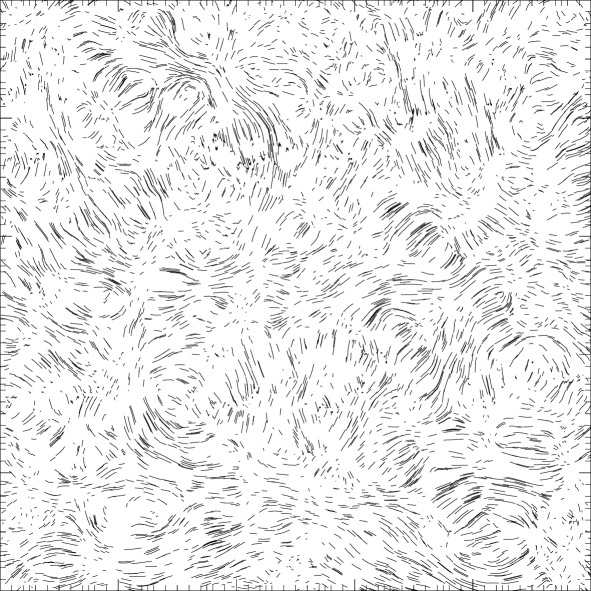
Figure 3: Example of shear map obtained from a numerical simulation (open CDM model, for an 5x5 square degree survey, van Waerbeke et al. 1999)

Fig. 2 shows the shear pattern expected for a power law spectrum of index $n=-1$ and for a matter three-point function shape given by the non-linear regime. The patterns observed around the pair points (located at positions [-1,0] and [1,0]) are rather complicated. In particular the circular shape expected around the pair points (according to the results of sect. 2.2.2) are observed only at very large distances (more that 5 times the pair separation). At separation comparable to the pair distance the patterns increase complexity, with a substantial part of the area with no significant correlation. The most striking feature is the quasi-uniform shear orientation along the segment joining the two-points. This effect which is indeed expressed in Eq. (46), where a uniform component is explicitly predicted, clearly strengthens in between the pair points. Such a feature might appear somewhat surprising but a close inspection of synthetic shear maps (Fig. 3) indeed reveals a lot of highly contrasted clumpy regions surrounded by strong coherent shear patterns primarily oriented transversely to directions between lumps.

The central pattern is the strongest and the most typical feature of the three-point correlation map and should be the easiest detectable one in the data. The previous analytical results suggest that such a structure is expected to hold for power law indices between $-2$ and $-1$ and should then be robust enough to be used as a detection tool of non-gaussianities. More detailed analysis performed along this idea are presented in the following.

3 Comparison with numerical simulations

Figure 4: The shear pattern of $\left\langle(\@vec{\gamma}({\@vec{x}}_{1}).\@vec{\gamma}({\@vec{x}}_{2})){\@vec{\gamma}}({\@vec{x}}^{\prime})\right\rangle$ measured in ray-tracing simulations (Jain et al., 2000) for increasing pair separation $|{\@vec{x}}_{2}-{\@vec{x}}_{1}|$. The separations are, from top to bottom and left to right, 2, 4, 6, and 8 in plot units (1 unit corresponds to about 10”). The pair points are along the horizontal axis.

The numerical simulations we use are described in Jain et al. (2000). The cosmological model is an open Universe ($\Omega_{{\rm m}}=0.3$, $\Omega_{\Lambda}=0$) with a Cold Dark Matter power spectrum ($\Gamma=0.21$) and a normalization $\sigma_{8}=0.85$. The sources are located at redshift unity and the simulation area covers about 11 square degrees with a resolution of $0.1$ arcmin.

The shear patterns for pair points at increasing separation is shown on (Figure 4). A visual inspection of their morphology and strength confirms that the uniform shear pattern within an ellipse that encompasses the pair points (as described in the next section) is likely an optimum way to extract non-gaussian signal. When the separation is small, the overall circular shear pattern is clearly visible. When the separation increases the shear appears uniform in the neighborhood of the segment joining the pair points, and is mostly radial at finite distance. We have already seen that these results might somewhat be dependent on the power spectrum index. For this simulation the index varies from $-1.3$ to $-1$ and it is thus natural that the patterns look like those obtained in case of a power-law model $n=-1$.

4 Improved measurement strategies

In this section we compare the measurements made in mock catalogs that mimic a large number of observational effects with different input models. We use these results to develop different survey strategies adapted to real data set.

4.1 Mock catalogues

The mock catalogues are generated from simulated sky images following the procedure described in Erben et al. (2001). The only difference here is that the galaxies are lensed according to a realistic cosmic shear signal, using ray-tracing simulations (Jain et al. 2000) instead of having a constant shear amplitude as in Erben et al. 2001. The galaxies are analyzed exactly in the same way as real data, following the procedure described in van Waerbeke et al. (2000, 2001b). In particular, the mock catalogues contain the main three features encountered in the actual surveys:

• galaxy intrinsic shape fluctuations;

• masks;

• noise from galaxy shape measurements and systematics from PSF corrections  ,

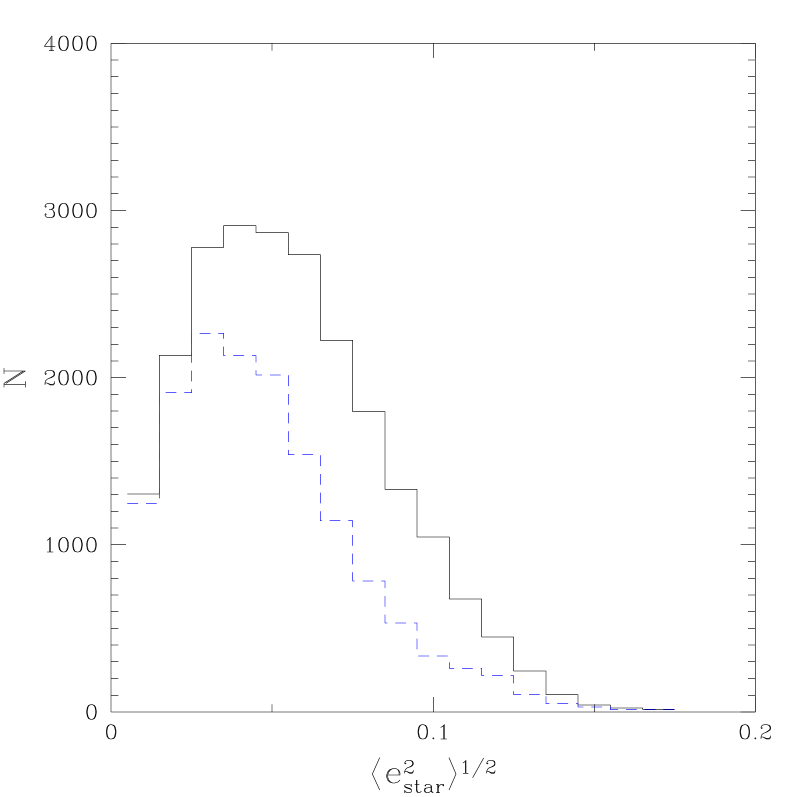
Figure 5: Histogram of the Point Spread Function anisotropy of the stars in the simulated images (solid line) and in the VIRMOS-DESCART survey (dashed line).

and the simulated images reproduce observational conditions matching our data set (PSF anisotropy, limiting magnitude, luminosity functions, galaxy and star number densities, intrinsic ellipticity…). The PSF anisotropy is even larger than the one in our data set, as shown in Figure 5, but it is uniform . We used two ray-tracing simulations from Jain et al. (2000): one is OCDM, as described in Section 3, and the other is a $\tau$CDM with $\Gamma=0.21$ and $\Omega_{{\rm m}}=1$. For each simulation we produced $11$ square degrees of simulated sky images containing roughly $30$ galaxies per arcmin², with a pixel size of $0.2$ arcsec. The galaxies are lensed following the ray-tracing shear before generating the image . In addition to the galaxy mock catalogues, we produced a reference catalogue containing only the cosmic shear values. We can therefore study separately the effect of masks, the ellipticity Poisson noise, real noise and systematics, when compared to the reference catalogue results.

4.2 Detection strategy

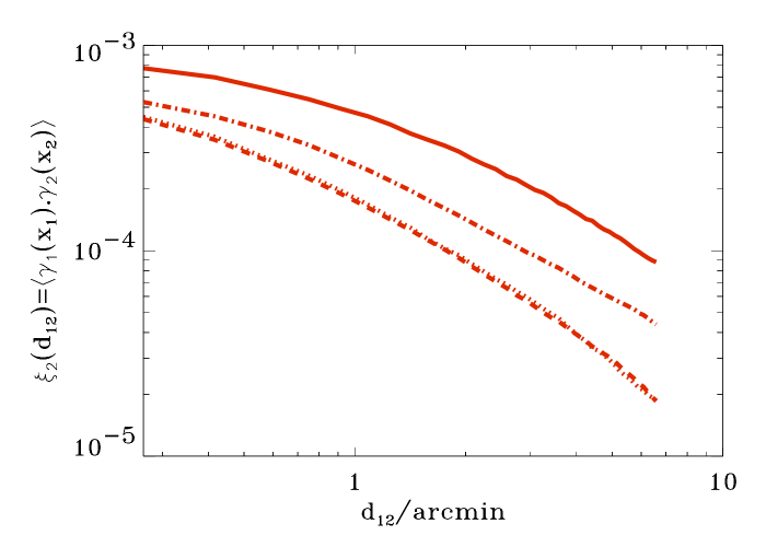
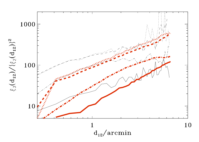
Figure 6: Results for the measured value of the two-point function and the reduced three-point function (as defined in Eq. 54) as a function of the pair distance for an Open CDM model (thick dashed lines) a $\Lambda$CDM (thick dot-dashed lines) and a $\tau$CDM model (thick solid lines). Results obtained in an Open CDM models with masks is shown as thick dotted lines. Galaxies in the catalogs have no intrinsic ellipticities. The measurements are made in bins of width 10”. The thin lines of the right panel corresponds to $200\,(n+2)/(-n)$, $150\,(n+2)/(-n)$ and $60\,(n+2)/(-n)$ for the open, $\Lambda$ and $\tau$ CDM case respectively, where $n$ is the power spectrum index measured from the slope of the corresponding two-point correlation functions.

The adopted strategy is to measure the two component quantity

$$\overline{\xi_{3}}(|{\@vec{x}}_{1}-{\@vec{x}}_{2}|)=\int_{\rm ellipse}{{\rm d}^{2}{\@vec{x}}^{\prime}\over V_{\rm ellipse}}\langle\left({\@vec{\gamma}}({\@vec{x}}_{1}).{\@vec{\gamma}}({\@vec{x}}_{2})\right)\,{\@vec{\gamma}}({\@vec{x}}^{\prime})\rangle$$ (54)

for different separations. The bar means we perform the average of $\langle\left({\@vec{\gamma}}({\@vec{x}}_{1}).{\@vec{\gamma}}({\@vec{x}}_{2})\right)\,{\@vec{\gamma}}({\@vec{x}}^{\prime})\rangle$ within the area defined by $V_{\rm ellipse}$. The ellipse properties are defined to cover an area that encompasses the pair points in which the orientation of the shear pattern is expected to be uniform. To be more specific, after some trials we have obtained a good balance between the signal intensity and the shot noise amplitude when the ellipse has a $0.4$ eccentricity, the pair points being its foci (see on Fig. 2).

The computation time can be reduced by building first a Delaunay triangulation (Delaunay, 1934; see also van de Weygaert, 1991) of the survey so that the neighbor list of any galaxy in the survey can be easily (and quickly) constructed. The quantity $\overline{\xi_{3}}(|{\@vec{x}}_{1}-{\@vec{x}}_{2}|)$ is a pseudo-vector, but its second component, e.g. the one corresponding to elongation at 45 degrees to ${\@vec{x}}_{1}-{\@vec{x}}_{2}$, vanishes in average for symmetry reasons. Therefore we only have to compute one component, which we define as,

$$\overline{\xi}^{\rm{\ t}}_{3}(d_{ij})={\sum_{ijk}w_{i}\,w_{j}\,w_{k}\,({\@vec{e}}_{i}.{\@vec{e}}_{j})\ e^{(ij)}_{k}\over\sum_{ijk}w_{i}\,w_{j}\,w_{k}}$$ (55)

where ${\@vec{e}}_{i}$ are the galaxy ellipticities, $e^{(ij)}_{k}$ is the tangential (e.g. first) component, with respect to the segment ${\@vec{x}}_{j}-{\@vec{x}}_{i}$, of the ellipticity of the galaxy of index $k$, $w_{i}$ are weights associated with each galaxy. The sums are made under the following constraints:

• $d_{ik}>d_{min}$, $d_{jk}>d_{min}$ so that close pairs are excluded to avoid spurious small angular scale signals (van Waerbeke et al. 2000) and

• $d_{ik}+d_{jk}<1.1\,d_{ij}$ so that galaxy $k$ is within the afore defined ellipse and the sum is splitted in bins according to the $d_{ij}$ distance.

We then plot the reduced three point function, that is $\overline{\xi}^{\rm{\ t}}_{3}$ in units of $[\xi_{2}(d_{ij})]^{2}$,

$$\xi_{2}(d_{ij})={\sum_{ij}w_{i}\,w_{j}\,({\@vec{e}}_{i}.{\@vec{e}}_{j})\over\sum_{ijk}w_{i}\,w_{j}}.$$ (56)

The noise is estimated by computing the r.m.s. of the estimator in small individual bins (for which the noise dominates the signal), and then rebinned in the final, larger, bins (as described in Pen et al., 2002). The noise of the reduced three-point function is computed assuming that the noise of the second and the third moments are uncorrelated. This might not be exact but the consequence of this assumption is insignificant since the main contribution to the noise of the ratio is in general the three-point moment.

4.3 Behavior of the reduced three-point function

In Fig. 6 we show the behavior of the reduced three-point function in the simulations. These simulations do not contain any noise, except that the shear field is measured in discrete randomly placed points. It is found to be a slowly growing function of scale. This might first appear surprising (this ratio is expected to be constant for a constant $Q$) but this result should be examined in the light of equation (39) and the subsequent comments: at small scale $n$ decreases, therefore it is expected that the reduced three-point function also decreases. Indeed, as demonstrated on the right panel of Fig. 6, the reduced ratio behaves approximately like $(n+2)/n$ at least for scale above 2’ with a multiplicative coefficient ($200$, $150$ and $60$ for respectively an open, $\Lambda$ and $\tau$ CDM model) that roughly correspond to the values of the convergence skewness $s_{3}$ at small scale in those models (Hui 1999).

On this plot the effects of masks on these quantities are shown as dotted lines. As expected its effect on the two-point function is null. Its effect on the three-point function as measured here is not totally absent (different configurations taken into account in Eq.(54) may have different weights when masks are taking into account). It appears however that it has a negligible effect compared to the other sources of noise.

Fig. 7 also shows the amplitude of the cosmic variance to be expected in an 11 square degree survey for the reduced three-point function and in case of an Open CDM model (dotted dashed lines). These error bars have been obtained from the results obtained in 7 realizations of the same model. They show that 30% fluctuation is to be expected in the signal. It is to be noted also that the error bars are correlated in the different bins.

4.4 Optimization and noise effects

A proper choice of weights $w_{i}$ is essential for getting a good signal to noise ratio. We have found that the introduction of a cut-off in the galaxy ellipticity distribution,

$$w_{i}\sim\exp\left(-{e_{i}^{2}\over 2\,e_{0}^{2}}\right)\ ,$$ (57)

improves the signal detection but may also affect its amplitude. In figure 7 a cut-off is introduced with $e_{0}=0.5$ in order to improve the S/N ratio. If the measured shear is simply the sum of the intrinsic shear and some noise,

$${\@vec{e}}_{i}={\@vec{\gamma}}({\@vec{x}}_{i})+\epsilon_{i}$$ (58)

then the cut in $e$ translates in a cut in $\gamma$ that can be simply described. The result depends on the shape of the intrinsic ellipticity PDF, $P(\epsilon)$,

$${\@vec{\gamma}}_{i}^{\rm cut}={\int{\rm d}^{2}{\@vec{\epsilon}}\ ({\@vec{\gamma}}({\@vec{x}}_{i})+\epsilon_{i})\,P(\epsilon)\,\exp\left(-{({\@vec{\gamma}}_{i}+{\@vec{\epsilon}})^{2}\over 2\,e_{0}^{2}}\right)\over\int{\rm d}^{2}{\@vec{\epsilon}}\,P(\epsilon)\,\exp\left(-{({\@vec{\gamma}}_{i}+{\@vec{\epsilon}})^{2}\over 2\,e_{0}^{2}}\right)}.$$ (59)

If the cut-off value $e_{0}$ is large enough compared to the typical excursion of cosmic shear values, then this equation can be linearized in $\gamma$ and one finds that,

$${\@vec{\gamma}}_{i}^{\rm cut}=f_{c}\,{\@vec{\gamma}}({\@vec{x}}_{i})+\ldots$$ (60)

with

$$f_{c}={\int\epsilon\,{\rm d}\epsilon\left(1-{\epsilon^{2}\over 2\,e_{0}^{2}}\right)\,P(\epsilon)\,\exp\left(-{\epsilon^{2}\over 2\,e_{0}^{2}}\right)\over\int\epsilon\,{\rm d}\epsilon\,P(\epsilon)\,\exp\left(-{\epsilon^{2}\over 2\,e_{0}^{2}}\right)}.$$ (61)

For the adopted ellipticity distribution and for $e_{0}=0.5$, the value of $f_{c}$ is about 0.8. Moreover the cut-off is large enough to have no impact on the non-gaussian properties of the shear field (e.g. sub leading order terms in Eq.(60) have a negligible effect).

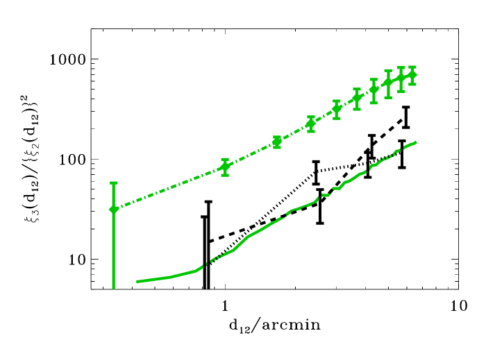
Figure 7: The reduced three-point function as in previous figure for different noise types in the catalogs. Error-bars for the open CDM model (dotted-dashed line) correspond to a cosmic variance estimation. The plot also compares the case of exact ellipticities for a $\tau$CDM model (solid lines) with the case where galaxies have intrinsic ellipticities (dotted lines, the measurement is made in 4 independent bins) and the case where noises in the shape determination are included (after PSF corrections, etc…, dashed lines, 4 bins). Error bars correspond here to measurement errors, not to the cosmic variance, and are therefore uncorrelated.

These numerical investigations are useful for exploring the effects of various noises. As expected the intrinsic ellipticities increase the noise, but do not bias the result. For $11$ square-degrees surveys the signal to noise for the detection in a $\tau$CDM model is still comfortable (see Fig. 7). Masking effects are also rather mild. They bias very weakly the results (see Fig. 6) and only slightly deteriorate the signal to noise ratio when intrinsic ellipticities are taken into account (because the number of available pairs or triplets is smaller).

Moreover, when similar measurements are made in mock catalogues that incorporate realistic noises we described above, we recover the expected signal with still a reasonable signal to noise ratio: it is still larger than 3 in 3 independent bins (see Fig. 7). Note that the S/N ratio for the reduced skewness is not only sensitive to the amplitude of the three point function, but also to the amplitude of the 2-point function. On the lower curves of Fig. 7, only the noise coming from the three-point function measurement is shown. Its amplitudeis roughly independent on the cosmological model (it scales basically like the inverse square root of the number of triplets available).

5 Conclusion

We have presented various geometrical patterns that the shear three-point correlation function is expected to exhibit. Its dependence with the cosmological parameters is found to be similar to that of the skewness of the convergence field, opening an alternative way to break the degeneracy between the amplitude of the density fluctuations, $\sigma_{8}$, and the density parameter of the Universe $\Omega_{{\rm m}}$. However, the reduced three-point function of the shear is more dependent on the power spectrum index than the skewness. In particular it is expected to vanish when the index gets close to $-2$. Numerical investigations have nonetheless proved the shear patterns to be robust enough to provide a solid ground for the detection of non-gaussian properties in cosmic shear fields.

We proposed a detection strategy that has been tested in mock catalogues that include realistic noise structures such as residual systematics and PSF anisotropy as seen in the real data. The quality of the PSF correction is always good enough to provide an accurate measurement of the shear three-point function. Since the mock catalogues were designed to reproduce the characteristics of the current VIRMOS-DESCART lensing survey, we conclude that non-gaussian signal should be detectable in this data set. The result of our investigations is presented in another paper (Bernardeau et al. 2002).

Beyond the detection, the scientific exploitation of the 3-point function for cosmology also depends on our ability to overcome other important difficulties. For instance, we found the cosmic variance amplitude to be of the order of 30% of the signal on the reduced three-point function, in agreement with previous studies made for the convergence. Other issues regarding source clustering, source redshift uncertainties, and intrinsic alignment of galaxies have not been considered here.

The measurement of non-gaussian signatures in lensing surveys is of course of great interest because it provides an independent measure of the mean mass density of the Universe in addition to test the gravitational instability paradigm which lead to large scale structures. It is likely that the analysis of cosmological non-gaussian signatures will be one of the major and most promising goals of emerging dedicated lensing surveys that take advantage of panoramic CCD cameras of the MEGACAM generation (Boulade et al 2000).

- (1)
- (2) Bacon, D.J., Refregier, A.R. & Ellis, R.S. 2000, MNRAS, 318, 625
- (3) Benabed, K. & Bernardeau, F. 2001, PRD, 64, 3501B
- (4) Bernardeau, F. 1995, A&A, 301, 309
- (5) Bernardeau, F. 1996, A&A, 312, 11
- (6) Bernardeau, F., van Waerbeke, L. & Mellier, Y. 1997, A&A 322, 1
- (7) Bernardeau F., Mellier, Y. & van Waerbeke, L. 2002, A&A in press. astro-ph/0201032
- (8) Bernardeau F., Colombi, S., Gaztanaga, E. & Scoccimarro, R., 2001, Phys. Rep. in press, astro-ph/0112551
- (9) Bernardeau, F. & Valageas, P. 2000, A&A, 364, 1
- (10) Boulade, O., Charlot, X., Abbon, P., et al. 2000, SPIE 4008, 657
- (11) Colombi, S., Bernardeau, F., Bouchet, F.R. & Hernquist, L. 1997, MNRAS 287, 241
- (12) Delaunay, B.N., 1934, Bull. Acad. Sci. USSR: Classe Sci. Mat, 7, 793
- (13) Erben, T., et al. 2001, A& A, 366, 717
- (14) Hui, L., 1999 ApJL, 519, 9
- (15) Jain, B. & Seljak, U. 1997, ApJ, 484, 560
- (16) Jain, B., Seljak, U. & White S. 2000, ApJ, 530, 547
- (17) Kaiser, N. 1992, ApJ 388, 272
- (18) Kaiser, N. 1998, ApJ, 498, 26
- (19) Kaiser, N., Squires G., Fahlman G. & Woods D. 1994, in ”Clusters of galaxies”, eds. F.Durret, A.Mazure & J.Tran Thanh Van, Editions Frontières.
- (20) Kaiser, N., Wilson, G. & Luppino, G. 2000, astro-ph/0003338
- (21) Limber, D. 1954, ApJ, 119, 655
- (22) Maoli, R. et al. 2001, A&A, 368, 766
- (23) Pen, U.-L., van Waerbeke, L. & Mellier, Y. 2002, ApJ, 567, 31
- (24) Schneider, P. 1996, MNRAS 283, 837
- (25) Schneider, P., van Waerbeke, L., Jain, B. & Kruse, G. 1998, MNRAS 296, 873
- (26) Scoccimarro, R. & Frieman, J.A. 1999, ApJ, 520, 35
- (27) Scoccimarro, R. & Couchman, H. 2001, MNRAS, 325, 1312
- (28) Stebbins, A. 1996, astro-ph/9609149
- (29) Tóth, G., Hollósi, J. & Szalay, A. S. 1989, ApJ 344, 75
- (30) van de Weygaert, R. 1991, Ph.D. thesis, Leiden University
- (31) van Waerbeke, L., Bernardeau, F. & Mellier, Y. 1999, A&A 342, 15
- (32) van Waerbeke, L. et al. 2000, A&A, 358, 30
- (33) van Waerbeke L., Hamana T., Scoccimarro R., Colombi S. & Bernardeau F. 2001a, MNRAS, 322, 918
- (34) van Waerbeke, L. et al. 2001b, A&A, 374, 751
- (35) Villumsen, J.V. 1996 MNRAS, 281, 369
- (36) Wittman, D.H., Tyson J.A., Kirkman, D., Dell’Antonio, I. & Bernstein, D. 2000, Nature, 405, 143