Wavelet tomography of the Galactic magnetic field

We suggest a two-dimensional wavelet devised to deduce the large-scale structure of a physical field (e.g., the Galactic magnetic field) from its integrals along straight paths from irregularly spaced data points to a fixed interior point (the observer). The method can be applied to the analysis of pulsar rotation and dispersion measures in terms of the large-scale Galactic magnetic field and electron density. The method does not use any á priori assumptions about the physical field and can be considered as an algorithm of wavelet differentiation. We argue that a certain combination of the wavelet transformation with model fitting would be most efficient in the interpretation of the available pulsar $\mathrm{RM}$ data.

1 Introduction

Tomography, understood broadly, is a reconstruction of a multidimensional physical field from its integral projections obtained by exposing it in different aspects. Tomography problems often occur in astronomy, especially radio astronomy, where the intervening medium is transparent and the observable quantities represent certain integrals along the line of sight. An important example is the studies of the magneto-ionic medium in the Milky Way using the Faraday rotation measure $\mathrm{RM}$ and dispersion measure $\mathrm{DM}$ of pulsars – both are integrals along the line of sight involving interstellar magnetic field and thermal electron density. A peculiar feature of the astronomical tomography is that just one vantage point is available, as the observer is confined to the close vicinity of the Sun. Astronomical tomography then focuses on extended objects which can be meaningfully analyzed using the integral projections obtained in a variety of directions.

In this paper we suggest a method to assess the spatial structure of the global Galactic magnetic field using pulsar $\mathrm{RM}$ (and also $\mathrm{DM}$ as the Faraday rotation measure depends on the thermal electron density), one of the most informative tracers of the large-scale component of the magnetic field (see e.g., Beck 2000). A fundamental problem here is that the derivation of magnetic field $\@vec{B}$ from the observable integral

$$\mathrm{RM}\equiv K\int_{0}^{r}n_{\mathrm{e}}{\@vec{B}}\cdot d{\@vec{s}}\;,$$ (1)

in fact involves differentiation of the observed quantity with respect to $r$ resulting in a catastrophic amplification of noise. Moreover, the distances to pulsars, $r$, are contaminates by large errors, both random and systematic. The problem is further aggravated by the fact that the pulsars (and extragalactic radio sources), that provide the $\mathrm{RM}$ data, are irregularly spaced and cover the sky very inhomogeneously. Here $n_{\mathrm{e}}$ is the number density of thermal electrons, $r$ is the distance to the radio source and $K=0.81\,{\rm rad\,m^{-2}\,cm^{3}\,\mu G^{-1}\,pc^{-1}}$; the positive direction of $\@vec{s}$ is that towards the observer, so that a field directed towards the observer produces positive $\mathrm{RM}$. The thermal electron density can be obtained from the dispersion measure of pulsars (Manchester 1972, 1974):

$$\mathrm{DM}\equiv\int_{0}^{r}n_{\mathrm{e}}\,ds\,,$$ (2)

and this involves similar complications.

The idea of this paper is twofold. Firstly, we use wavelets to filter out the noise in the $\mathrm{RM}$ data resulting from small-scale fluctuations in the magneto-ionic medium and from the irregular spacing of the data points. Secondly, we introduce a new, specialized family of wavelets devised to avoid (or at least to minimize) noise amplification in dealing with an observable represented by an integral along the line of sight, given that the available data probe a range of distances into the field localization region. The Faraday rotation and dispersion measures of pulsars are suitable observables for such an analysis.

The plan of the paper is as follows. In Sect. 2 we discuss the available samples of pulsar $\mathrm{RM}$ and $\mathrm{DM}$ and methods used to obtain $\@vec{B}$ and $n_{\mathrm{e}}$ from them. Section 3 introduces the basic ideas of our method, which can be applied in various contexts. The algorithm is described in Sect. 4, and the advantages and limitations of the method are discussed in Sect. 5. The efficiency of the method when applied to the pulsar $\mathrm{RM}$ is discussed in Sect. 6.

2 Obtaining magnetic field from RM and electron density from DM

Faraday rotation measures of pulsars probe the Galactic magnetic field in a variety of directions. A pulsar’s own contribution to the observed $\mathrm{RM}$ is minor because the pulsar magnetosphere is populated by electron-positron pairs resulting in zero net Faraday rotation. This makes pulsars a major source of information about the large-scale magnetic field of the Milky Way (e.g., Rand & Kulkarni 1989; Rand & Lyne 1994), especially in conjunction with their dispersion measures. However, there are several complications in the derivation of magnetic field and electron density from pulsar $\mathrm{RM}$ and DM.

Figure 1: The 323 pulsars with known $\mathrm{RM}$ from the catalogue of Taylor et al. (1995) are shown in the galactic plane. Here and below, scale is given in kiloparsecs and the Galactic centre is shown with cross; the Sun is at the centre of the frame.

Firstly, pulsars are very non-uniformly distributed in space. They concentrate in spiral arms and the number density of known pulsars decreases rapidly with distance from the Sun as shown in Fig. 1. Even though the number of known pulsars rapidly grows with time, the non-uniform nature of their spatial distribution remains. Most pulsars are found near the Galactic midplane. Yet, some of them are located far away from the midplane, and thereby allow a study of the vertical distribution of the magneto-ionic medium. Nevertheless, in this paper we restrict ourselves to a two-dimensional analysis by projecting the pulsar data onto the galactic plane; our method can be generalized to three dimensions, but better data would be needed to justify this.

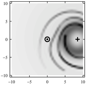
Figure 2: The thermal electron density $n_{\mathrm{e}}$ distribution in the Galactic plane, following the model of Taylor & Cordes (1993), with the Galactic centre marked with cross and the Sun at the centre of the frame. Darker shades of grey correspond to larger densities.

Secondly, the electron density can be obtained from dispersion measures only if the distance to the pulsars is known. Distance estimates now exist for a few hundreds of pulsars, resulting from three basic techniques: neutral hydrogen absorption (in combination with the Galactic rotation curve), trigonometric parallax and from associations with objects of known distance (Lorimer 2001). The distance of a pulsar can be obtained from $\mathrm{DM}$ if the distribution of $n_{\mathrm{e}}$ is known. Taylor & Cordes (1993), based mainly on the scintillation and dispersion measure data, have suggested an electron density model expected to provide distance estimates with an average uncertainty of about $30\%$. However, distances to individual pulsars may be as wrong as by as a factor of two (e.g., Johnston et al. 2001).

The method suggested here can be applied to pulsar dispersion measures to obtain thermal electron density using pulsars with known distances. Then magnetic field can be obtained from $\mathrm{RM}$ using the same method. However, dispersion measures alone are not sufficient to obtain a reliable distribution of $n_{\mathrm{e}}$, and a model for the electron density should be used in order to derive magnetic field distribution from Faraday rotation measures.

The largest catalogue of pulsars contains 706 objects (Taylor et al. 1995). Faraday rotation and dispersion measures, together with the distances are known for only 323 of them.

The simplest estimate of the line of sight component of the large-scale magnetic field $\@vec{B}$ can be obtained by dividing $\mathrm{RM}$ by $\mathrm{DM}$. This would be justified if both $\@vec{B}$ and $n_{\mathrm{e}}$ were uniform along the line of sight, which is definitely not the case. A more elaborate analysis involves a pair of pulsars located close to each other in the sky, so $n_{\mathrm{e}}$ between the two pulsars can be obtained from the increments in $\mathrm{DM}$ and $r$ as $n_{\mathrm{e}}\simeq\Delta\mathrm{DM}/\Delta r$. Then the longitudinal magnetic field follows as $B_{||}\simeq\Delta\mathrm{RM}/(K\Delta n_{\mathrm{e}})$. However, $\Delta r$ is most often too large to make the resulting estimate reliable. The nature of the problem is intrinsically related to that arising in differentiating unevenly sampled data (cf. Ruzmaikin et al. 1988, p. 34). A possible resolution is to use multivariate statistical analysis where a model for magnetic field is adopted and its parameters are obtained by fitting (Ruzmaikin et al. 1988; Rand & Kulkarni 1989; Rand & Lyne 1994). A disadvantage of this (and any other) analysis of this kind is that one has to impose á priori model restrictions on the structure of the magnetic field. Furthermore, it is often difficult, if not impossible, to get convincing evidence that the model adopted is compatible with observations because errors in the observable quantities are rarely known confidently and this hampers the application of statistical tests for the quality of the fit. Here we attempt at developing a method of field reconstruction from the integrals (1) and (2) which allows us to avoid these shortcomings. Our method is based on wavelet analysis.

3 The wavelet analysis

The data similar to those presented in Fig. 1 obviously would not allow one to reconstruct the field in all details. What is possible, however, is to reveal structures whose scale is larger than the size of the gaps between the points observed. For this purpose, one should separate large-scale structures from noise resulting not only from statistical errors but also from the irregular data grid. Recently wavelets have become an efficient tool for signal analysis, especially useful in scale separation problems. The main idea of this approach is a decomposition of the signal over a basis of self-similar functions, known as wavelets, that are localized in both physical and Fourier space. The wavelet transform can be considered as a generalization of the Fourier transform, which allows the derivation of the local spectral properties of the signal. Comprehensive reviews of the wavelet analysis can be found in Farge et al. (1993); Grossmann & Morlet (1984); Holschneider (1995).

In terms of the polar coordinates $(r,\varphi)$, the continuous two-dimensional wavelet transform (also known as the wavelet coefficient) of a function $F(r,\varphi)$ is given by

$$w(a,r,\varphi)={1\over\sqrt{a}}\int\limits_{-\pi}^{\pi}\!\!\int\limits_{0}^{\infty}\psi_{a,r,\varphi}(r^{\prime},\varphi^{\prime})F(r^{\prime},\varphi^{\prime})\,r^{\prime}\,dr^{\prime}\,d\varphi^{\prime},$$ (3)

where $\psi_{a,r,\varphi}(r^{\prime},\varphi^{\prime})$ is a family of wavelets characterized by position in the physical space ($r$,$\varphi$) and the scale $a$ which can be identified with the radius of the region where $\psi_{a,r,\varphi}(r^{\prime},\varphi^{\prime})=O(1)$. A self-similar family of wavelets is generated from an ‘analyzing wavelet’ $\Psi(r,\varphi)$ by translation and dilation. Many various wavelets have been suggested. The success of wavelet analysis depends on appropriate choice of the wavelet $\Psi(r,\varphi)$. Most importantly, some wavelets provide better resolution if the wave number (Fourier) space (at the expense of the localization information), whereas others are advantageous if higher spatial resolution is needed (but then the scale separation power can be only modest). The wavelet used here derives from an isotropic wavelet known as the ‘Mexican hat’, which has good resolution in the physical space,

$$\Psi(x)=\left(2-x^{2}\right)\exp{\left(-{\textstyle{1\over 2}}x^{2}\right)}\;,$$ (4)

where $x$ is the distance from the wavelet center. An isotropic wavelet has no preferred direction, and so rotation is not included into the transformations generating the wavelet family, which is defined as

$$\psi_{a,r,\varphi}(r^{\prime},\varphi^{\prime})={1\over{a}}\Psi\left({s(r,\varphi,r^{\prime},\varphi^{\prime})\over{a}}\right)\;,$$ (5)

where $s(r,\varphi,r^{\prime},\varphi^{\prime})$ is the distance between the $(r,\varphi)$ (the centre of the wavelet) and the current point $(r^{\prime},\varphi^{\prime})$.

Ideally, wavelet analysis consists of decomposing the signal into contributions from a range of scales, filtering out the smaller scales dominated by noise and the reconstruction of the filtered signal (presumably free of noise) using the inverse wavelet transform. However, this procedure is rarely followed completely because this would require observational data of unrealistically high quality. Instead, we shall consider the wavelet coefficients themselves, but at a scale distinguished by the data. Specifically, we focus on those scale(s) which make a dominant contribution to the ‘spectral energy density’ (see below). The wavelet coefficients form a three-parametric family. For representation and interpretation purposes, we shall usually consider a set of two-dimensional maps of $w(a,r,\varphi)$ for a fixed $a$.

A useful integral diagnostic of the importance of different scales in the data is the wavelet spectrum, defined as

$$M(a)=\int\limits_{-\pi}^{\pi}\!\!\int\limits_{0}^{\infty}w^{2}(a,r,\varphi)\,r\,dr\,d\varphi\;.$$ (6)

In the Fourier analysis, a similar quantity is known as the spectral energy density. The normalization factor in Eq. (5) is chosen so that structures of the same amplitude (but different scales) contribute equally to $M(a)$.

4 Wavelet differentiation

In this section we suggest a general method to analyze an observable represented by an integral, with variable limit(s), of the physical field whose reconstruction is the goal of the analysis. Deriving magnetic field from pulsar $\mathrm{RM}$ is a perfect example of such a problem, however the method can be used in many other problems of image analysis. The main idea of the method is to avoid the differentiation of the discrete, noisy data. Instead, we differentiate the wavelet itself, which is given in an analytical form. Thus, the algorithm can be considered as a sort of wavelet interpolation used to derive the derivative of an observable quantity.

4.1 The differentiating wavelet

Let $F(r,\varphi)$ be an unknown function whose integral

$$G(r,\varphi)=\int\limits_{0}^{r}F(r^{\prime},\varphi)\,dr^{\prime}\;,$$ (7)

is known for various values of $r$. In the context of this paper, $G(r,\varphi)$ can be $\mathrm{DM}$ or $\mathrm{RM}$ (and $F(r,\varphi)$ is related to $n_{\mathrm{e}}$ or $n_{\mathrm{e}}B_{\parallel}$, respectively), and the origin of the reference frame is at the solar position.

The exact expression for $F$ involves a derivative of $G$, $F(r,\varphi)={\partial G(r,\varphi)}/{\partial r}$. Since $G$ is known only at discrete data points, one has to use a smooth interpolation of $G$ in order to derive $F(r,\varphi)$. Random and systematic noise makes this procedure unstable. This difficulty also arises in standard tomography problems where a two-dimensional function is reconstructed from its integral projections contaminated by noise (Patrickeyev & Frick 1999).

Wavelet analysis can help to alleviate this problem. Given Eq. (7), one can rewrite Eq. (3) as

$$w(a,r,\varphi)={1\over{\sqrt{a}}}\!\int\limits_{-\pi}^{\pi}\!\int\limits_{0}^{\infty}\!\psi_{a,r,\varphi}(r^{\prime},\varphi^{\prime})\frac{\partial G(r^{\prime},\varphi^{\prime})}{\partial r^{\prime}}\;r^{\prime}\,dr^{\prime}\,d\varphi^{\prime}.$$ (8)

Integrate by parts to obtain

$$w(a,r,\varphi)=-{1\over{\sqrt{a}}}\int\limits_{-\pi}^{\pi}\!\!\int\limits_{0}^{\infty}\overline{\psi}_{a,r,\varphi}(r^{\prime},\varphi^{\prime})G(r^{\prime},\varphi^{\prime})r^{\prime}\,dr^{\prime}d\varphi^{\prime},$$ (9)

where $\overline{\psi}_{a,r,\varphi}(r^{\prime},\varphi^{\prime})$ is a new wavelet family related to the original wavelet by

$$\overline{\psi}_{a,r,\varphi}(r^{\prime},\varphi^{\prime})=\frac{\partial\psi_{a,r,\varphi}(r^{\prime},\varphi^{\prime})}{\partial r^{\prime}}+\frac{\psi_{a,r,\varphi}(r^{\prime},\varphi^{\prime})}{r^{\prime}}\;.$$ (10)

Here we have taken into account that $G(0,\varphi)=0$ and that the wavelet is localized in the physical space,

$$\lim\limits_{r^{\prime}\to\infty}r^{\prime}\psi_{a,r,\varphi}(r^{\prime},\varphi^{\prime})=0\;.$$ (11)

Altogether, we have introduced a new family of wavelets that allows us to reconstruct $F(r,\varphi)$ without differentiating the data. The forms of the ‘Mexican hat’ and the associated differentiating wavelet are illustrated in Fig. 3. Unlike the ‘Mexican hat’, the differentiating wavelet is not isotropic, and has two zeros.

Figure 3: (a) The ‘Mexican hat,’ Eq. (4), and (b) the associated differentiating wavelet, Eq. (10). In this illustration, the wavelets are centered at $(r,\varphi)=(5,0)$ and have the scale $a=2$. The zero-level contours are shown solid and the dashed contours corresponds to the magnitude of 1% of the maximum. Darker shades of grey correspond to larger values.

The new wavelet $\overline{\psi}$ has zero mean value,

$$\int\limits_{-\pi}^{\pi}\!\int\limits_{0}^{\infty}\overline{\psi}_{a,r,\varphi}(r^{\prime},\varphi^{\prime})\,r^{\prime}\,dr^{\prime}d\varphi^{\prime}=0\;,$$ (12)

and so satisfies what is known as the admissibility condition. Another admissibility condition is that

$$\int\limits_{-\pi}^{\pi}\!\int\limits_{0}^{\infty}\overline{\psi}_{a,r,\varphi}(r^{\prime},\varphi^{\prime})\,r^{\prime 2}\,dr^{\prime}d\varphi^{\prime}=0\;.$$ (13)

Equations (12) and (13) imply that the wavelet coefficients are independent of a constant component of $G(r,\varphi)$ and its linear trend, respectively, – a behavior required for any wavelet in order to have an inverse transformation. Thus, $F(r,\varphi)$ can be determined up to a constant background value proportional to the value of $B_{\parallel}$ at $r=r_{\rm max}$, where $r_{\rm max}$ is the distance to the most remote pulsar. If $r_{\rm max}$ is large enough, this background value is close to zero.

4.2 Implementation for irregularly spaced data

The calculation of the integral (9) on a discrete, irregular data grid is not straightforward. The need for a robust numerical algorithm is especially demanding since the separation of pulsars in the available catalogues is often comparable to or exceeds the physically interesting scales of the large-scale Galactic magnetic field. The difficulties becomes crucial if the separation of the data points can be comparable to the scale of the wavelet, $a$.

In our case, a convenient method to calculate the integrals is the Monte-Carlo technique, leading to

$$w(a,r,\varphi)=-{\Delta S(a,r,\varphi)\over{\sqrt{a}}}\sum_{i=1}^{N}\overline{\psi}_{a,r,\varphi}(r^{\prime}_{i},\varphi^{\prime}_{i})\,G(r^{\prime}_{i},\varphi^{\prime}_{i})\,r^{\prime}_{i}\,,$$ (14)

where $N$ is the number of data points for $G(r,\varphi)$ and $\Delta S$ is the average area element of an individual data point. For a uniform distribution of the data points, $\Delta S$ is a constant, but this is not true for a non-homogeneous distribution. We chose $\Delta S$ (a function of position and the scale of the wavelet, identified with the effective weight of data points) as to minimize the error arising from the non-uniform distribution of the data points. The contribution of a data point to the integral sum (14) must be small if the point is far away from the centre of the wavelet, $\@vec{r}^{\prime}$, as compared with the scale of the wavelet, $a$, so that we take

$$\Delta S(a,r,\varphi)=a^{2}\left[{\sum_{i=1}^{N}\Phi\left({s(r,\varphi,r_{i},\varphi_{i})\over{a}}\right)}\right]^{-1}\,.$$ (15)

The value of $a^{2}/\Delta S$ gives the approximate number of sample points within the wavelet localization area. So, $a^{2}/\Delta S$ should be large enough in order to achieve sufficient accuracy.

Another problem arising in the numerical realization of the wavelet transformation is the necessity to satisfy the admissibility conditions (12) and (13) with sufficient accuracy. We use for this purpose the gapped (or adaptive) wavelet technique (see Frick et al. 1998) wherein the ‘analyzing wavelet’ is represented in the form

$$\Psi(x)=h(x)\Phi(x)\;,$$ (16)

where $\Phi(x)$ is a positive definite function that determines the position of the wavelet (the envelope). For the ‘Mexican hat’, Eq. (4), $\Phi(x)=\exp(-{\textstyle{1\over 2}}x^{2})$ and $h(x)=2-x^{2}$. The main idea of the technique is to modify $h(x)$ in order to satisfy the two conditions (12) and (13). This can be achieved by introducing two quantities $C_{1}$ and $C_{2}$, functions of scale $a$ and position $(r,\varphi)$, such that

$$\Psi(x)=[h(x)+C_{0}+C_{1}x]\Phi(x)\;.$$ (17)

These functions are determined from the discrete versions of Eqs. (12) and (13) for each scale $a$ and wavelet position $(r,\varphi)$.

5 Testing the method

In order to assess the possibilities of the method, we consider a test function $F(r,\varphi)=n_{\mathrm{e}}$ similar to that of the Milky Way Taylor & Cordes (1993). We first calculate the corresponding values of $G(r,\varphi)\propto\mathrm{DM}(r,\varphi)$ using Eq. (1) and then apply our method to obtain $F(r,\varphi)$ from $G(r,\varphi)$ on a selection of data grids.

Figure 4: (a) The test function $F$ and (b) the corresponding distribution of $G$ calculated from $F$ using Eq. (7). With $F=n_{\mathrm{e}}$, $G$ is proportional to $\mathrm{DM}$. Lighter shades of grey correspond to smaller values.

We show in the upper panel of Fig. 4 a test function $F=n_{\mathrm{e}}$ that includes an annular and spiral structures with characteristic scales (transverse half-widths) $a=3\,$kpc and $a=1\,$kpc, respectively. This distribution in similar to (but not identical with) that of Fig. 2. The lower panel of Fig. 4 shows the corresponding $G=\mathrm{DM}(r,\varphi)$ calculated in the whole plane.

The quality of the reconstruction of $F$ from $G$ obviously depends on how well $G$ is sampled. For a reliable reconstruction of a simple, isotropic isolated object whose structure is similar to that of the wavelet itself, one needs at least 10 data points within it. Then one would need about 2000 data points distributed uniformly in $(r,\varphi)$ in order to detect structures of the smallest scale of 1 kpc in the $20\,\mbox{kpc}\times 20\,\mbox{kpc}$ Solar vicinity. However, Faraday rotation measures are only known for about 300 pulsars; furthermore, their distribution is very non-uniform being very sparse beyond 3–5 kpc from the Sun, especially in the fourth Galactic quadrant. Thus, the available pulsar data can only yield reliable information about structures in a narrower vicinity of the Sun and/or at a scale of a few kiloparsecs.

Now we consider a series of wavelet transforms on different data grids, from an ‘ideal’ to a realistic case through an ‘acceptable’ one.

Figure 5: The wavelet transform of the distribution of Fig. 4b on a regular $40\times 40$ grid at a scale (a) $a=3\,$kpc (the scale of the annulus) and (b) $a=1\,$kpc (the scale of the spirals).

A regular grid is the best for the calculation of the integral (9). The data point separation of $0.5\,$kpc (needed to recover structures at a scale of 1 kpc) requires a sample of 1600 points. The wavelet transforms of the distribution of Fig. 4 sampled on a regular grid of 1600 points are shown in Fig. 5 for the scales $a=3\,$kpc and $1\,$kpc. As expected, the annular structure is better pronounced at $a=3\,$kpc (Fig. 5a) and the spirals are better visible at $a=1\,$kpc (Fig. 5b). Figures 5a and b together reproduce the distribution of Fig. 4 reasonably well, demonstrating the possibilities of the wavelet transform in scale separation. However, the scale resolution of the wavelet, derived from the ‘Mexican hat’, is only modest, and this contaminates the wavelet transform at $a=3\,$kpc with a trace of the spiral arms, and that at $a=1\,$kpc with a weak signature of the annulus. The magnitude of the wavelet coefficient is maximum when the scale of the wavelet is equal to the scale of the structure. The integral wavelet spectrum $M(a)$, defined in Eq. (6) and shown in Fig. 6 confirms that the scales $1\leq a\leq 3$ are dominant in $G(r,\varphi)$, but they are not separated from each other.

Figure 6: The integral wavelet spectrum $M(a)$ for the distribution of Fig. 4b, sampled on a regular $40\times 40$ grid, with $a$ in kpc.

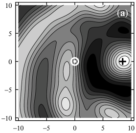
(a)  (b)

Figure 7: The wavelet transforms of the distribution of Fig. 4b sampled at 1600 randomly distributed points at the scales (a) $a=3\,$kpc and (b) $a=1\,$kpc.

Figure 8: The wavelet transform of the distribution of Fig. 4b on the real, irregular data grid of the pulsar catalogue of Taylor et al. (1995) (323 points) at a scale $a=1.5\,$kpc. The region where $\Delta S>a^{2}/5$ and the results are inaccurate is filled with uniform grey.

Further, we consider the data of Fig. 4b sampled at the same number of points (1600), but now the data points are scattered randomly and statistically uniformly in the same region $20\,\mbox{kpc}\times 20\,\mbox{kpc}$ around the Sun. The distortions in the resulting wavelet transform maps of Fig. 7 are significant even though the two basic components of the distribution are clearly recognizable. The structures in the wavelet transform become patchy, especially at small scales, because of the large gaps in the data grid.

Finally, the wavelet transform on the data grid of the pulsar catalogue of Taylor et al. (1995) (using only the positions of 323 pulsars with known $\mathrm{RM}$) is shown in Fig. 8. The data points are crowded within 3 kpc from the Sun. We consider the wavelet transform to be unreliable where $\Delta S>a^{2}/5$; these regions are marked with uniform grey shade in Fig. 8. The spiral arms segments of the original distribution of Fig. 4a is recognizable in the 3 kpc vicinity of the Sun, but they appear patchy and discontinuous. The annulus at the galactocentric distance of 4 kpc is hardly visible at all, and the arm-interarm contrast is overestimated.

6 Discussion

We have introduced a new wavelet devised for the analysis of the pulsar Faraday rotation measures in terms of the large-scale magnetic field (or of any other observable that is an integral of the quantity studied, e.g., the pulsar dispersion measures). This is a tomography approach because the field is directly reconstructed from its integral estimator. The method works well with data given on a regular mesh or scattered randomly but with gaps between the data points not exceeding $a/2$, with $a$ the scale of the wavelet. The separation of pulsars with known $\mathrm{RM}$ exceeds this limit beyond about 3 kpc from the Sun.

An advantage of the method is that it involves neither ad hoc assumptions about magnetic field structure nor model fitting. However, the wavelet transforms on the data grid of the pulsar catalogues available appear rather confusing and difficult to interpret. The advantages of the wavelet analysis and model fitting can be combined in a single approach applied by Frick et al. (2001) to the Faraday rotation measures of extragalactic sources. Instead of fitting a magnetic field model to noisy $\mathrm{RM}$ data, these authors fitted the wavelet transform of the model $\mathrm{RM}$ to the wavelet transform of the observed $\mathrm{RM}$ with smaller scales (mainly responsible for the nose) filtered out. This has resulted in a significant improvement in the quality of the analysis. The application of the wavelet introduced here will allow us to fit the wavelet transforms of the magnetic field derived from $\mathrm{RM}$ to the model. We expect that will result in a significant improvement of the results against the usual procedure of fitting model $\mathrm{RM}$ to the observed noisy data.

Another way to improve the results would be to analyze simultaneously the Faraday rotation measures of pulsars and extragalactic radio sources. Since many extragalactic sources occur at high Galactic latitudes, a plausible assumption about the vertical distribution of the magneto-ionic medium will have to be adopted.