Massive molecular outflows

With the aim of understanding the role of massive outflows in high-mass star formation, we mapped in the ¹²CO $J=2-1$ transition 26 high-mass star-forming regions at very early stages of their evolution. At a spatial resolution of $11^{\prime\prime}$ bipolar molecular outflows were found in 21 of them. The other five sources show confusing morphology but strong line wings. This high detection rate of bipolar structure proves that outflows common in low-mass sources are also ubiquitous phenomena in the formation process of massive stars. The flows are large, very massive and energetic, and the data indicate stronger collimation than previously thought. The dynamical timescales of the flows correspond well to the free-fall timescales of the associated cores. Comparing with correlations known for low-mass flows, we find continuity up to the high-mass regime suggesting similar flow-formation scenarios for all masses and luminosities. Accretion rate estimates in the $10^{4}$ L_⊙ range are around $10^{-4}$ M_⊙yr^-1, higher than required for low-mass star formation, but consistent with high-mass star formation scenarios. Additionally, we find a tight correlation between the outflow mass and the core mass over many orders of magnitude. The strong correlation between those two quantities implies that the product of the accretion efficiency $f_{\rm{acc}}=\dot{M}_{\rm{acc}}/(M_{\rm{core}}/t_{\rm{ff}})$ and $f_{\rm{r}}$ (the ratio between jet mass loss rate and accretion rate), which equals the ratio between jet and core mass ($f_{\rm{acc}}f_{\rm{r}}=M_{\rm{jet}}/M_{\rm{core}}$), is roughly constant for all core masses. This again indicates that the flow-formation processes are similar over a large range of masses. Additionally, we estimate median $f_{\rm{r}}$ and $f_{\rm{acc}}$ values of approximately 0.2 and 0.01, respectively, which is consistent with current jet-entrainment models.
To summarize, the analysis of the bipolar outflow data strongly supports theories which explain massive star formation by scaled up, but otherwise similar physical processes – mainly accretion – to their low-mass counterparts.

1 Introduction

Molecular outflows are a well known phenomenon in sites of low-mass star formation, and they play an important role in transporting angular momentum away from the forming star. The observational database on low-mass outflows has increased tremendously over the last decade, giving rise to different formation scenarios. While it is still unclear how the outflow is accelerated near the proto-star and/or disk, it is now widely believed that low-mass molecular flows are momentum driven by highly collimated jets, which entrain the surrounding molecular gas. For recent reviews on this topic see, e.g., Richer et al. (2000); Bachiller & Tafalla (2000); Shu et al. (2000); Königl & Pudritz (2000).

The situation in the high-mass star formation regime is less clear, because, due to the rarity of these objects and the typically larger distances (a few kpc) of sites of high-mass star formation, the spatial resolution has been lacking to resolve the outflows and their driving sources properly. Recent systematic molecular line studies of high-mass outflows have been carried out by Shepherd & Churchwell (1996a, b); Henning et al. (2000); Zhang et al. (2001); Ridge & Moore (2001). All of them find that $\sim 90\%$ of the observed massive star-forming regions are associated with high velocity gas. Mapping a subsample of 10 sources (out of 94) Shepherd & Churchwell (1996b) find bipolar morphology in 5 of them and Zhang et al. (2001) found spatial outflow structures in 39 of 69 sources. Thus, both studies indicate bipolar structures in at least $50\%$ of the observed sources.

Including more massive outflow sources from the literature, the overall picture has emerged, that outflows are ubiquitous phenomena in massive star formation, that they are very massive (up to hundreds of solar masses in the flows), very energetic ($\sim 10^{46}$ erg) but seemingly not very collimated (i.e. collimation factors – the length of the flow divided by its width – between 1 and 10 for low-mass sources versus collimation factors between 1 and 1.8 for high-mass sources, Richer et al. 2000; Churchwell 2000b; Ridge & Moore 2001). The high masses in the flows as well as the low collimation factors, which are difficult to explain in current jet-entrainment scenarios, have given rise to new ideas of outflow formation including the possibility that massive outflows consist of accelerated gas which has been deflected by the young accreting proto-star, rather than swept-up ambient material (Churchwell, 2000b). Devine et al. (1999) propose a slightly different scenario in which massive stars produce collimated jets only in their earliest phases, and with increasing luminosity of the central objects the jets may be replaced by wide-angle winds.

To test the proposed scenarios it is necessary to increase the number of outflow sources using a homogenous sample with adequate angular resolution. Therefore, we mapped 26 promising candidates from a larger sample of massive star formation sites in the $J=2\to 1$ line of CO with the 30 m telescope at a spatial resolution of $11^{\prime\prime}$. This work is part of a long term project to search and investigate 69 massive and rather isolated star formation regions in an evolutionary stage prior to building significant ultracompact Hii regions. An introduction to the sample and first results are given in Sridharan et al. (2002) and Beuther et al. (2002a).

In the following, we present the observed dataset and give a detailed analysis of the outflow characteristics. The derived parameters are compared with those from low-mass as well as other high-mass outflows, and we discuss the implications for star formation in such regions.

2 Observations

2.1 Source Selection

The 26 sources observed in this study were chosen from a sample of 69 high-mass proto-stellar candidates based on the CO 2–1 line wings seen by these authors in pointed observations (Sridharan et al., 2002). We do not believe that there was a particular bias in this selection. Sridharan et al. (2002) found wings in 85 percent of their sample and argue on the basis of the statistical distribution of inclination angles that essentially all of these sources are associated with outflows. As also argued by Sridharan et al. (2002), the majority of this sample is likely to be young and 50 percent have no associated 9 GHz radio continuum flux down to a limit of 1 mJy. This suggests they have not had time to form a substantial Hii region. While the low radio continuum flux may have a variety of causes (e.g., high 9 GHz optical depth or dust mixed with ionized gas), we consider the sample of sources observed by us to be an arbitrarily chosen set of very young regions of high-mass star formation.

2.2 IRAM 30 m observations

The IRAM 30 m telescope on Pico Veleta near Granada (Spain) was used to map 26 sources in the $J=2-1$ transition of ¹²CO in April and November 1999 and in April 2000. Maps with an average extent of $100^{\prime\prime}\times 100^{\prime\prime}$ were observed in the on-the-fly mode, where the telescope moves continously across the source and dumps the data in a well chosen grid. At 230.5 GHz the resolution of the 30 m telescope is approximately $11^{\prime\prime}$. Beuther et al. (2000) have shown that Nyquist-sampling is sufficient in the on-the-fly mode as well, because the beam is smeared out by only about $4\%$. Therefore we chose as a sampling interval $4^{\prime\prime}$ (Nyquist interval $\theta_{Ny}=\frac{\lambda}{2D}\sim 4.5^{\prime\prime}$). The dump time was 2 sec per position and we scanned all maps twice, in most cases in perpendicular directions to reduce scanning effects. Experience showed that the whole system (weather+technical system, $T_{\rm{sys}}\sim 250$ K) is stable for around 5 minutes. Therefore our ON-OFF cycles never exceeded that time. OFF positions were chosen based on the Stony Brook and the CfA-survey of the galactic plane (Sanders et al., 1986; Dame et al., 2001) and checked to be emission free. The frequency resolution was 0.1 km/s and the beam efficiency 0.41.

The data were reduced with CLASS and GRAPHIC of the GILDAS software package by IRAM and the Observatoire de Grenoble. To improve the signal to noise ratio, the ¹²CO data are smoothed to a velocity resolution of 1 km/s, sufficient to sample the broad CO lines.

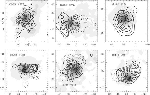
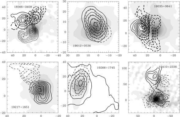
Figure 1: Massive molecular outflows: the solid lines show the blue wings and the dashed lines the red wings of CO 2–1 emission. The contours are chosen to highlight the most prominent features in each source, usually between $30\%$ and $90\%$ (steps of $10\%$) of the peak integrated wing intensity. The dotted lines in 18566+0408 represent an additional feature at “blue” velocities [58,60] km/s. The grey scale presents the corresponding 1.2 mm continuum maps from $5\%$ and $95\%$ by steps of $10\%$ of the peak flux as outlined in Beuther et al. (2002a). The axis show offsets in arcsec from the absolute IRAS-positions given in Sridharan et al. (2002). Detailed morphological descriptions are given in Sect.3.1 .

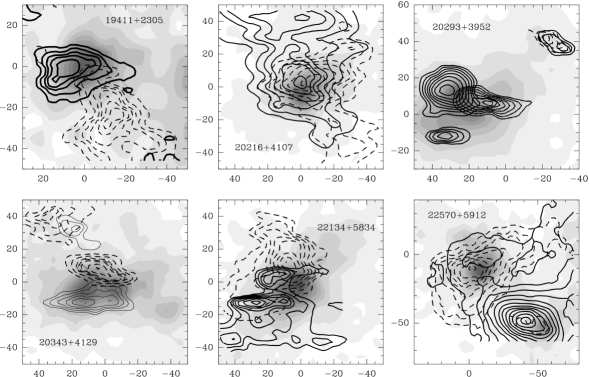
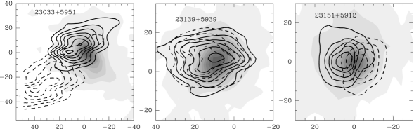
Figure 1: continued. The red wing for the southern flow in 20293+3952 is missing due to instrumental problems in that region, but simultaneously observed SiO data (not presented here) confirm this southern flow.

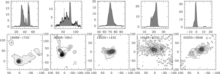
Figure 2: For sources without clear bipolar outflow structure we show the summed ¹²CO 2–1 spectra ($\rm{T_{mb}}$ [K] versus velocity [km/s]) corresponding to the regions outlined by the 1.2 mm continuum maps in grey scale. The continuum images are presented as in Fig. 1 .

3 Observational results

3.1 Morphologies

Fig. 1 presents the outflow sources [CO 2–1 blue (solid lines) and red wing emission (dashed lines) overlayed on the grey scale 1.2 mm continuum maps (Beuther et al., 2002a)]. From the 26 sources observed, 21 show either bipolar morphology or wide non–Gaussian line wings such that we suspect the outflow is along the line of sight (23139+5939) and not spatially resolvable with the $11^{\prime\prime}$ resolution of our observations. The 5 remaining sources ($18089-1732$, $18308-0841$, $19220+1432$, $19413+2332$ and $20205+3948$) also show line wings, but the maps are very chaotic, so that we could not define any outflow structure. All the sources are in the galactic plane (Sridharan et al., 2002) and unrelated spiral arm emission is partly confusing the spectra. Fig. 2 presents for “confused” sources the sum of all spectra in the regions outlined by the 1.2 mm dust maps (Beuther et al., 2002a). We cannot tell if the latter are a superposition of many flows, or if they are more isotropic flows, similar to that observed in Orion (Rodriguez-Franco et al., 1999; Schultz et al., 1999). This can only be investigated with higher angular resolution in the future but we note that most of our sample is less luminous than Orion IRC2 ($L\sim 2\times 10^{5}\leavevmode\nobreak\ \rm{L}_{\odot}$, Churchwell 2000b). Within the range of luminosities which we sample (roughly $10^{3.5}$ to $10^{5}$ L_⊙), we find that bipolar features are omnipresent. We also do not observe a statistical difference in finding bipolar outflow structures for sources with or without detected cm emission suggesting perhaps that the arrival of proto-stars on the ZAMS is not critical for the outflow.

All the mapped sources showed wing emission in previous single pointing observations conducted at the 30 m telescope (Sridharan et al., 2002). Therefore we expected outflows in all sources, but the large fraction with bipolar structures ($\sim 80\%$) is rather surprising. Previous mapping studies of massive molecular outflows found bipolar structures only in approximately $50\%$ of the sources (Shepherd & Churchwell, 1996a; Zhang et al., 2001), which seemingly suggested that bipolarity is less probable in high-mass than in low-mass star formation (Churchwell, 2000b). The high detection rate of bipolar outflows in our study is most likely due to the improved spatial resolution of our data ($11^{\prime\prime}$) compared to previous statistical work on massive outflows (compare radius $r$ in Table 1 to $60^{\prime\prime}$ resolution in Shepherd & Churchwell (1996b) and $30^{\prime\prime}$ in Zhang et al. (2001)).

Every outflow is associated with massive mm cores (grey-scale in Figure 1). It is not evident that the size of the flows depends on the size of the cores: about $50\%$ of the flows have an extent larger than the mapped core sizes, whereas the other half of the flows are smaller. In most cases, the flows are centered on the mm peak, which most likely harbors the most massive and youngest proto-stars. But there are a few remarkable exceptions, where the flows are centered offset from the mm peak (18566+0408, 19035+0641, 19217+1651, 19411+2305, 22570+5912). The reasons for such offsets are not clear. For 18566+0408 and 19035+0641, pointing problems may be the explanation since simultaneously observed H¹³CO⁺ 1–0 maps (not published so far) peak approximately at the center of the flows and offset relative to the mm cores. In the cases of the more chaotic looking flows 19411+2305 and 22570+5912, this seems unlikely and the structure may be due to several low-mass flows, which are not at the center of the mm core.

19217+1651 on the other hand is not chaotic but a nice examples of a bipolar outflow which makes a superposition of several low-mass flows very unlikely. Additionally, the offset between the flow center and the single dish outflow map is real because H¹³CO⁺ 1–0 as well as thermal CH₃OH (both observed simultaneously with the outflow) peak at the mm core. Using a theoretically derived correlation between the momentum of the outflow and the proto-stellar mass (Eq. 18 in Tan & McKee (2002)), we can infer a mass for the proto-star powering the outflow. In this way, we conclude that the proto-star has a mass of at least 10 M_⊙. This suggests that high-mass proto-stars can emerge from the core where they were formed. The projected offset between the flow center and the mm peak is of order 0.3 pc which implies a relatively high peculiar velocity of the proto-star relative to the core ($\sim 4$ km/s) using the flow timescale given in Table 2. This is obviously an object of considerable interest and interferometric observations with the Plateau de Bure Interferometer are currently being conducted.

The flows are rather large with an average size of $\sim 0.8$ pc (see Table 2). The collimation factors derived for this sample are higher than previously claimed. Richer et al. (2000) in their review note that so far no massive flow with a collimation factor $f_{\rm{c}}$ larger than 1.8 has been observed. The last column of Table 1 presents the collimation factors we derive for our sample (flows with a question mark are along the line of sight, which makes a determination of $f_{\rm{c}}$ difficult). These collimation factors are lower limits due to angular resolution and projection effects, but we nevertheless obtain a mean $f_{\rm{c}}$ of 2.1, larger than most measurements of high-mass flows to date. The largest $f_{\rm{c}}$ we find in the single dish data is 3, but we know from interferometric observations of selected sources that $f_{\rm{c}}$ can be even higher: $f_{\rm{c}}\sim 10$ for 05358+3543 (Beuther et al., 2002b) and $f_{\rm{c}}\sim 5$ for 23033+5951 (Wyrowski et al., in prep.). It is interesting to compare the observed collimation factors with theoretical expectations: a flow at 5 kpc (the mean distance of this sample) extended 1 pc in length and 0.1 pc in width results in an intrinsic $f_{\rm{c}}=10$. Inclination effects to first order just reduce the length of the flow but not the widths; thus the length has to be corrected on the average by $\cos(57^{\circ})$ (mean inclination angle). After converting the linear scales into arcseconds and convolving with an $11^{\prime\prime}$ beam – as for our CO data  – the length of the flow is $\sim 25^{\prime\prime}$ and the width $\sim 12^{\prime\prime}$, resulting in an observable $f_{\rm{c}}=2.1$, which is similar to the mean value we derive for our sample. Thus, the observed collimation factor is a strong function of the available angular resolution and high-mass flows may in general be as well collimated as flows from low-mass proto-stars (though see the discussions of Devine et al. (1999) and Reipurth & Bally (2001)). Even this new dataset with $11^{\prime\prime}$ resolution underestimates collimation factors; higher resolution with interferometers is needed for that.

In 4 fields (18151$-$1208, 19410+2336, 20293+3952, 20343+4129) we see at least two separated flows. Interferometric data for two of the flows (05358+3543 Beuther et al. 2002b; 23033+5951 Wyrowski et al., in prep.) reveal that those single dish flows split up into at least two outflows, but the data also show that most of the single dish flux ($>50\%$ for 05358+3543 and $>80\%$ for 23033+5951) is produced by one major flow with minor contributions from the second flow. There are likely to be multiple lower-mass flows, and recent theoretical studies by Tan & McKee (2002) consider massive outflows to be a superposition of outflows from all proto-stars of each cluster evolving simultaneously. This scenario results in less collimated flows and may explain some of our more chaotic sources, but it does not seem to be applicable in general. Thus, contributions from lower-mass flows are possible, but the high degree of collimation and bipolarity we find on average in addition to that found in a small number of sources with interferometric observations strongly suggest that our data are dominated by the most massive outflow of each cluster.

3.2 Characteristics of the outflows

The determination of outflow parameters is subject to a large number of errors. To first order, it is difficult to separate the outflowing gas from the ambient gas, and the inclination angles of the flows are also often unknown. Cabrit & Bertout (1986, 1990, 1992) performed a series of studies on outflows from low-mass sources and the approach we are following here is outlined in Cabrit & Bertout (1990). The velocity range due to the outflow is determined in two ways. One is to define the flow by the line wings in the spectra, the other approach is to map each channel and decide from the spatial separation of different channels, which belong to an outflow and which correspond to the ambient core emission. In some sources both criteria were suitable, in other sources only one of them, e.g., the 05358+3543 flow is known to be near the plane of the sky (Beuther et al., 2002b) causing us to use the spatial separation. A counter example is 23139+5939, which shows extremely strong wing emission but nearly no lobe separation probably due to being rather along the line of sight (Fig. 1). Then we mapped the chosen wings, and the size of the flow (transformed to linear scales, size_b & size_r) and the mean value of integrated wing emission ($\int T_{\rm{mb}}(^{12}\rm{CO}2-1)$, mean_b & mean_r) were used as inputs to the flow calculations. Additional input parameters are the radius $r$ of the flow from the projected center, and the maximum velocity separation of the red and the blue wings $v_{\rm{max_{r}}}$ & $v_{\rm{max_{b}}}$. All the input parameters are presented in Table 1. An additional uncertainty is caused by distance ambiguity in which cases the outflow parameters are calculated for the near and the far distance (Table 2).

Table 1: Parameters for outflow calculations: The number of flows per source #, the infrared luminosity $L$ derived from the HIRES-data (Sridharan et al., 2002) (if the kinematic ambiguity is unresolved both values – near and far – are given), the velocity range of the wings $\Delta v$, the mean of the integrated wing emission, the maximum projected velocity $v_{\rm{max}}$ and the radius $r$ of the flow. The last column presents the collimation factor $f_{\rm{c}}$

source	#	$L$	$\Delta v_{\rm{b}}$	$\Delta v_{\rm{r}}$	meanb	meanr	$v_{\rm{max_{b}}}$	$v_{\rm{max_{r}}}$	$r$	$f_{\rm{c}}$
		[log(L⊙)]	[km/s]	[km/s]	[km/s K]	[km/s K]	[km/s]	[km/s]	[′′]
05358+3543	1	3.8	($-$32,$-$21)	($-$12,$-$4)	28.5	29.7	14.4	13.6	60	2.0
18151$-$1208	1	4.3	(25,30)	(38,42)	20.2	12.2	5	10	45	2.1
18182$-$1433	1	4.3/5.1	(53,56)	(62,70)	26.5	26.1	6.1	12	25	1.7
18264$-$1152	1	4.0/5.1	(28,37)	(52,63)	38.4	46.6	16	18	20	?
18345$-$0641	1	4.6	(82,90)	(102,106)	28.6	16.8	14	10	40	1.5
18470$-$0044	1	4.9	(86,91)	(102,106)	24.3	9.0	10.5	9.5	38	2.0
18566+0408	1	4.8	(68,77)	(96,102)	15.2	9.2	17	17	40	2.4
19012+0536	1	4.2/4.7	(55,62)	(70,75)	39.6	21.6	10	10	30	?
19035+0641	1	3.9	(21,27)	(38,43)	12.0	4.2	11	11	30	?
19217+1651	1	4.9	($-$16,$-$3)	(9,21)	31.4	26.2	19.5	17.5	28	2.8
19266+1745	1	1.7/4.7	($-3,0$)	(10,15)	15.4	5.4	8	10	35	?
19410+2336	1	4.0/5.0	(1,17)	(26,45)	35.3	64.0	21.4	22.5	43	2.0
19410+2336	2	4.0/5.0	(1,17)	(26,45)	36.0	52.0	21.4	22.5	45	2.1
19411+2306	1	3.7/4.3	(15,25)	(35,43)	32.4	27.0	14	14	35	2.3
20216+4107	1	3.3	($-$9,$-$4)	(1,6)	30.8	28.8	6.6	8.2	32	?
20293+3952	1	3.4/3.8	($-$16,4)	(12,25)	25.6	61.6	26	30	32	2.7
20293+3952	2	3.4/3.8	($-$16,4)	(12,25)	18.2	3.4	26	30	15	?
20343+4129	1	3.5	(8,9)	(13,15)	24.6	33.4	3.5	4.5	23	1.0
20343+4129	2	3.5	(8,9)	(13,15)	9.2	12.0	3.5	4.5	25	1.7
22134+5834	1	4.1	($-$30,$-$23)	($-$14,$-$4)	10.6	34.4	11.7	14.3	37	?
22570+5912	1	4.7	($-56,-50$)	($-42,-32$)	20.8	17.8	10	14	60	?
23033+5951	1	4.0	($-$67,$-$60 )	($-$47,$-$33)	21.8	34.2	14.0	19.4	50	3.0
23139+5939	1	4.4	($-$59,$-$47)	($-$39,$-$31)	43.0	23.6	11.1	13.2	29	?
23151+5912	1	5.0	($-89,-65$)	($-47,-35$)	53.8	11.8	34	19	20	1.2

Opacity corrected H₂ column densities $N_{\rm{b}}$ and $N_{\rm{r}}$ in both outflow lobes can be calculated by assuming a constant ¹³CO/¹²CO 2–1 line wing ratio throughout the outflows (Cabrit & Bertout, 1990). Choi et al. (1993) found an average ¹³CO/¹²CO 2–1 line wing ratio around 0.1 in 7 massive star-forming regions, which we adopt for our sample as well. Levreault (1988) found similar values in low-mass outflows. The derived flow parameters are the masses $M_{\rm{b}}$, $M_{\rm{r}}$ in the blue and red outflow lobes and the total mass $M_{\rm{out}}$, the momentum $p$, the energy $E$, the size, the characteristical time scale $t$ (radius of the flow $r$ divided by the flow velocity), the mass entrainment rate of the molecular outflow $\dot{M}_{\rm{out}}$ (as opposed to the mass loss rate of the jet $\dot{M}_{\rm{jet}}$), the mechanical force $F_{\rm{m}}$ and the mechanical luminosity $L_{\rm{m}}$ for each flow. For details see Cabrit & Bertout (1990). The used Eqs. are (assuming $\rm{H}_{2}/^{13}\rm{CO}=89\times 10^{4}$ (Cabrit & Bertout, 1992) and $T_{\rm{ex}}=30$ K; $m_{\rm{H_{2}}}$ is the mass of the H₂ molecule):

$$N = \left(\frac{\rm{H}_{2}}{{}^{13}\rm{CO}}\right)\left(\frac{\int T_{\rm{mb}}(^{13}\rm{CO}2-1)}{\int T_{\rm{mb}}(^{12}\rm{CO}2-1)}\right)\frac{3k^{2}T_{\rm{ex}}}{4\pi^{3}h\nu^{2}\mu^{2}}$$ (2)

$$\times\leavevmode\nobreak\ e^{-16.6/T_{\rm{ex}}}\int T_{\rm{mb}}(^{12}\rm{CO}2-1)$$

$$M_{\rm{out}} = (N_{\rm{b}}\times\rm{size_{b}}+N_{\rm{r}}\times\rm{size_{r}})\ m_{\rm{H_{2}}}$$ (3)

$$p = M_{\rm{b}}\times v_{\rm{max}_{b}}+M_{\rm{r}}\times v_{\rm{max}_{r}}$$ (4)

$$E = \frac{1}{2}M_{\rm{b}}\times v_{\rm{max}_{b}}^{2}+\frac{1}{2}M_{\rm{r}}\times v_{\rm{max}_{r}}^{2}$$ (5)

$$t = \frac{r}{(v_{\rm{max}_{b}}+v_{\rm{max}_{r}})/2}$$ (6)

$$\dot{M}_{\rm{out}} = \frac{M_{\rm{out}}}{t}$$ (7)

$$F_{\rm{m}} = \frac{p}{t}$$ (8)

$$L_{\rm{m}} = \frac{E}{t}$$ (9)

In the case of 18151$-$1208, we just determined the characteristics for the eastern flow, because the western one is confused by ambient emission. The derived quantities are shown in Table 2. Cabrit & Bertout (1990) state the mass determinations to be correct within approximately a factor 2, while kinematic parameters should be approximately correct within a factor 10. It is clear however from the Choi et al. (1993) study that the high opacity in ¹²CO transitions can lead to large errors for individual objects and it would be useful to obtain ¹³CO data for these sources. While several of the derived parameters are discussed in detail in §4, we want to stress that all of the observed sources show massive and energetic molecular outflows compared to low-mass flows (Richer et al., 2000).

Table 2: Outflow results: distances $D$ [kpc], number of outflows #, column densities $N$ [log₁₀(cm^-2)], masses $M_{\rm{b}}$ (blue), $M_{\rm{r}}$ (red) and $M_{\rm{out}}$ ($M_{\rm{out}}=M_{\rm{b}}+M_{\rm{r}}$) [$M_{\odot}$], momentum $p$ [$M_{\odot}$ km/s], energy $E$ [$10^{46}$erg], size [pc], time $t$ [$10^{4}$yr], mass entrainment rate $\dot{M}_{\rm{out}}$ [$10^{-4}$M_⊙/yr], mechanical force $F_{\rm{m}}$ [$10^{-3}$M_⊙km/s/yr] and mechanical luminsoity $L_{\rm{m}}$ [$L_{\odot}$]

source	$D$	#	$N_{\rm{b}}$	$N_{\rm{r}}$	$M_{\rm{b}}$	$M_{\rm{r}}$	$M_{\rm{out}}$	$p$	$E$	size	$t$	$\dot{M}_{\rm{out}}$	$F_{\rm{m}}$	$L_{\rm{m}}$
05358+3543	1.8	1	21.1	21.2	11	10	21	288	4.0	0.52	3.7	5.6	7.9	9.1
18151-1208	3.0	1	21.0	20.8	8	4	12	106	0.9	0.65	7.1	1.7	1.5	1.1
18182-1433	11.7	1	21.1	21.1	130	73	203	1665	15.0	1.42	15.3	13.0	11.0	8.2
18182-1433	4.5	1	21.1	21.1	19	11	30	246	2.3	0.55	8.9	3.4	2.8	2.1
18264-1152	12.5	1	21.3	21.4	234	171	405	6818	110	1.21	7.0	58.0	98.0	135.0
18264-1152	3.5	1	21.3	21.4	18	13	31	534	9.0	0.34	3.7	8.6	14.0	20.0
18345-0641	9.5	1	21.1	20.9	103	40	143	1841	24.0	1.84	15.0	9.5	12.0	13.1
18470-0044	8.2	1	21.1	20.6	86	16	102	1050	11.0	1.51	14.8	6.9	7.1	6.0
18566+0408	6.7	1	20.9	20.7	25	7	32	540	9.1	1.30	7.5	4.3	7.2	10.0
19012+0536	8.6	1	21.3	21.0	105	29	134	1339	13.0	1.25	12.2	11.0	11.0	8.9
19012+0536	4.6	1	21.3	21.0	30	8	38	383	3.8	0.67	13.0	2.9	2.9	2.4
19035+0641	2.2	1	20.8	20.3	2	1	3	28	0.3	0.32	2.9	0.9	1.0	0.9
19217+1651	10.5	1	21.2	21.1	38	70	108	1961	36.0	1.43	7.5	14.0	26.0	38.8
19266+1745	10.0	1	20.9	20.4	17	18	35	311	2.8	1.70	18.4	1.9	1.7	1.3
19266+1745	0.3	1	20.9	20.4	0.02	0.02	0.04	0.3	0.003	0.05	1.0	0.03	0.03	0.02
19410+2336	6.4	1	21.2	21.5	92	1331	1423	31896	710	1.33	5.9	240	540	982.9
19410+2336	2.1	1	21.2	21.5	10	143	153	3434	77.0	0.44	3.8	40.0	90.0	165.3
19410+2336	6.4	2	21.2	21.4	96	77	173	3766	82.0	1.40	6.2	28.0	61.0	108.3
19410+2336	2.1	2	21.2	21.4	10	8	18	405	8.8	0.46	4.0	4.6	10.0	18.2
19411+2306	5.8	1	21.2	21.1	19	28	46	649	9.0	0.98	6.9	6.7	9.4	10.8
19411+2306	2.9	1	21.2	21.1	5	7	12	162	2.3	0.49	6.9	1.7	2.4	2.7
20216+4107	1.7	1	21.2	21.1	3	3	6	43	0.3	0.26	3.5	1.7	1.3	0.8
20293+3952	2.0	1	21.1	21.5	2	7	9	270	7.8	0.31	1.1	8.6	25.0	59.2
20293+3952	1.3	1	21.1	21.5	1	3	4	114	3.3	0.20	1.3	3.0	8.7	20.6
20293+3952	2.0	2	20.9	20.2	1	0.1	1.1	21	0.6	0.15	0.5	1.6	4.2	9.1
20293+3952	1.3	2	20.9	20.2	0.3	0.1	0.4	8	0.2	0.09	0.6	0.6	1.5	3.2
20343+4129	1.4	1	21.1	21.2	1	1	2	9	0.04	0.16	3.8	0.6	0.2	0.1
20343+4129	1.4	2	20.7	20.8	0.2	0.2	0.4	1	0.007	0.17	4.2	0.1	0.04	0.01
22134+5834	2.6	1	20.7	21.2	2	15	17	242	3.4	0.47	3.5	4.9	6.9	7.9
22570+5912	5.1	1	21.0	20.9	30	43	73	911	11.0	1.48	12.1	6.1	7.5	7.8
23033+5951	3.5	1	21.0	21.2	9	23	32	566	10.0	0.85	5.0	6.4	11.0	16.9
23139+5939	4.8	1	21.3	21.1	41	16	57	662	7.7	0.67	5.4	10.0	12.0	11.7
23151+5912	5.7	1	21.4	20.8	13	8	21	597	18.0	0.55	2.0	10.0	29.0	72.7

Another important result from our study concerns the derived flow timescales $t$. These are likely to represent a lower limit to the true age of the flows (see Parker et al. 1991) and hence also to the time over which the embedded proto-stars responsible for the flows have been accreting from their surroundings. One can compare these estimates for the outflows with the free-fall times ($t_{\rm{ff}}=\sqrt{\frac{3\pi}{32G\rho}}$) derived from the mean gas density $\rho$ in the cores from which presumably the accretion takes place. $\rho$ is derived from the dust continuum maps as discussed by Beuther et al. (2002a). The free-fall times are an estimate of the timescale for dynamical evolution of the core and in fact theoretical studies of core evolution suggest that the timescale for star formation in a core is of order a few free-fall times (e.g., Tan & McKee 2002). Our comparison of $t$ and $t_{\rm{ff}}$ is shown in Fig. 3. We see that flow timescales and free-fall timescales are of the same order of magnitude and range for our sample between $2\times 10^{4}$ and $2\times 10^{5}$ years with an average dispersion about a factor 2 (for the sources with known distance). The rough equality between these independently derived quantities is surprising and it will be important to check whether this also holds for other samples. We tentatively conclude that for the present sample, flow ages are good estimates of proto-star lifetimes and will assume this in the following discussion.

Figure 3: Dynamical outflow times $t$ versus free-fall times $t_{\rm{ff}}$. The circles show sources with known distance whereas triangles represent sources with unresolved distance ambiguity (open triangle: near distance, filled triangle: far distance).

4 Discussion

4.1 High-mass versus low-mass outflows

We wish first of all to compare our results to systematic studies conducted in the low-mass regime. The analysis used for the low-mass flows discussed by Cabrit & Bertout (1992) and Bontemps et al. (1996) is very similar to ours and is based on results of Cabrit & Bertout (1990). Hence, we can usefully compare our data with those results.

Figure 4: Outflow parameter correlations: (a) mechanical force from CO versus core mass from 1.2 mm dust emission. (b) mechanical force versus bolometric luminosity. The dots represent our sample without distance ambiguity, the open triangles sources at near kinematic distance and the filled triangles sources at the far kinematic distance. The pentagons show data from Bontemps et al. (1996) and the squares data from Cabrit & Bertout (1992). Open squares and pentagons represent class I sources and filled symbols class 0 sources.

Fig. 4 shows the relations between the mechanical force $F_{\rm{CO}}$, the core mass $M_{\rm{core}}$ and the bolometric luminosity $L$. $F_{\rm{CO}}$ is derived from $F_{\rm{m}}$ (Table 2) by applying an inclination correction. Because we do not know the inclination for each source separately we apply a mean correction factor of 3, which corresponds to a mean inclination angle of $57.3^{\circ}$ (Bontemps et al., 1996). The main result of this comparison is that well established energetic correlations for low-mass outflows show a continuity up to the high-mass regime. A similar correlation was already presented by Lada (1985).

The low-mass data can be divided into class 0 and class I sources, and Fig. 4(b) suggests tentatively that the energetic parameters in the high-mass regime correlate better with class I sources. This might be interpreted as an indication that maybe no proper class 0 stage exists for massive stars. But clearly this proposition has to be checked for larger samples to draw firm conclusions.

Nevertheless, the continuity between the low-mass and the high-mass regime is strongly suggestive of an outflow formation mechanism which is present both in the low-mass as well as in the high-mass case.

4.2 Mass entrainment and accretion rates

Fig. 5 presents an update of the mass entrainment rate versus bolometric luminosity plot presented initially by Shepherd & Churchwell (1996b). In addition to our data we also include the massive outflow database compiled by Churchwell (2000b). Although the spread in the literature data is larger than for our more homogenous sample the mean of both is similar. This updated plot shows that the relation fitted by Shepherd & Churchwell (1996b) to the data of Cabrit & Bertout (1992) is just an upper envelope in the high-mass regime. The data indicate that the mass entrainment rate for sources $>1000$ L_⊙ does not depend strongly on the luminosity, and has an average $\dot{M}_{\rm{out}}=\rm{d}M_{\rm{out}}/\rm{d}t$ of $7.5\times 10^{-4}$ M_⊙yr^-1 with a spread between $10^{-4}$ M_⊙yr^-1 and $10^{-3}$ M_⊙yr^-1 (these numerical values are calculated just for our sample). While part of the non-correlation between $\dot{M}_{\rm{out}}$ and $L$ at high luminosities is certainly due to a variety of observational uncertainties, we believe that much of the dispersion is real. One must remember that while outflows in low-mass star formation regions can usually be identified with a given proto-star, in the regions of high-mass star formation studied here, we presumably deal with a cluster of embedded objects. It is possible that in some of our regions, for example, the most luminous object is on the ZAMS and has started nuclear burning whereas the most massive outflow emanates from a less evolved object. Proving this however will require higher angular resolution and comparison with VLA data.

Figure 5: Mass entrainment rates versus luminosities (from Sridharan et al. 2002). The dots (no distance ambiguity), open and filled triangles (near and far kinematic distance, respectively) show the data presented in this paper, the squares represent the data compiled from Churchwell (2000b) and the asterisks the data from Cabrit & Bertout (1992). The dotted line shows the second order polynomial fit to the data of Cabrit & Bertout (1992) as proposed by Shepherd & Churchwell (1996b).

More interesting than the mass entrainment rates are the accretion rates $\dot{M}_{\rm{acc}}$ of such massive objects. Regarding the flows as momentum driven the momenta of the observed outflow and the internal jet entraining the outflow should be conserved, if there is efficient mixing at the jet/molecular gas interface assuming no loss of momentum to the ISM (Richer et al., 2000):

$$p_{\rm{flow}}=M_{\rm{out}}v_{\rm{out}}=\dot{M}_{\rm{jet}}v_{\rm{jet}}t=p_{\rm{jet}}.$$ (10)

The mean value $v_{\rm{flow}}$ of the observed $v_{\rm{max}}$ (Table 1) is $\sim 15$ km/s. Correcting this by a mean inclination angle of $57^{\circ}$ (multiply by $1/\cos(57^{\circ})$) results in a molecular outflow velocity of approximately 28 km/s. This is still a lower limit because we are noise-limited, and material at higher velocities is likely.

Jet velocities from high-mass proto-stars have only been determined in a few cases. Marti et al. (1998) observe from proper motions jet velocities $v_{\rm{jet}}$ of a young massive star around 500 km/s, and Eislöffel et al. (2000) report that values between 500 km/s and 1000 km/s are typical. Based on this we assume in the following a mean ratio between jet velocity and molecular outflow velocity around 20, which results in jet masses $M_{\rm{jet}}$ and mass loss rate of the jets $\dot{M}_{\rm{jet}}$ about an order of magnitude below the rates of the entrained gas. Assuming further a ratio between mass loss rate of the jet and accretion rate of approximately 0.3 (Tomisaka, 1998; Shu et al., 1999), we get a mean accretion rate of $\sim 10^{-4}$ M_⊙yr^-1 for sources in the $10^{4}$ L_⊙ regime ; the distribution is shown in Figure 6. For the most luminous sources ($\sim 10^{5}$ L_⊙) listed by Churchwell (2000b) the accretion rates get as high as $10^{-3}$ M_⊙yr^-1. Such values are extremely high compared with typical accretion rates established for low-mass star formation ($10^{-6}-10^{-5}$ M_⊙yr^-1, Shu 1977). High mass accretion rates moreover ease the problem of overcoming radiation pressure and are required in order to form massive stars within a free-fall time (Jijina & Adams, 1996). It will be useful to examine the birth-line for such high accretion rates in more detail (see, e.g., Stahler et al. 2000; Norberg & Maeder 2000).

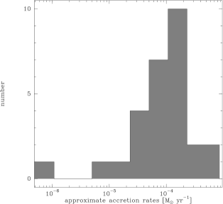
Figure 6: Histogram of the estimated accretion rates for our sample.

Other interpretations are still possible, and we cannot rule out that the chaotic sources without clear outflow structure could be generated by interacting proto-stars. Collisions of proto-stars are expected to be very energetic (Stahler et al., 2000) causing either real explosions during stellar merger, or in less dramatic scenarios they could significantly affect the rotation axis of the proto-stellar disks and thus cause strong precession of the outflows. But bipolar outflows are very difficult to explain in massive star formation scenarios based on the coalescence of proto-stars (Bonnell et al., 1998; Stahler et al., 2000). In contrast, high accretion rates as found in this study give strong support to theories, which explain massive star formation mainly by accretion analogous to low-mass scenarios albeit with accretion rates which are significantly higher. The fact that highly collimated and massive flows are found (this work and studies with higher resolution by Beuther et al. (2002b) and Wyrowski et al. in prep.) supports the proposition that the physical processes in the low- as well as the high-mass regime are similar.

4.3 Outflow mass versus core mass

We find a good correlation between the outflow mass $M_{\rm{out}}$ and the core mass $M_{\rm{core}}$ derived from the 1.2 mm dust emission (Beuther et al., 2002a), which is presented in Fig. 7 (left). Our best fit over more than 3 orders of magnitude in core mass is $M_{\rm{out}}\sim 0.1\cdot M_{\rm{core}}^{0.8}$. The ratio $M_{\rm{out}}/M_{\rm{core}}$ is rather constant with an average of 0.04 for the sources (Figure 7 right) and a spread of less than one order of magnitude. Thus, approximately $4\%$ of the core gas is entrained in the molecular outflow. There is a trend in our data that the ratio $M_{\rm{out}}/M_{\rm{core}}$ decreases with rising core mass $M_{\rm{core}}$, but the statistics at the upper mass end are too low for a definite conclusion on this point.

Figure 7: The left plot shows the molecular outflow mass versus core mass (Beuther et al., 2002a), whereas the right plot presents the ratio of both quantities versus the core mass. The circles show sources with no distance ambiguities, the filled and open triangles represent sources with far and near distances, respectively.

From the correlation between outflow and core mass, we estimate the accretion efficiency $f_{\rm{acc}}$. As discussed in §3.1 the derived parameters include contributions from several flows, but they are most likely dominated by one massive flow (see also the discussion in Tan & McKee 2002), and we neglect effects due to multiple sources in the following. We define $f_{\rm{acc}}$

$$f_{\rm{acc}}=\frac{\dot{M}_{\rm{acc}}}{M_{\rm{core}}/t_{\rm{ff}}}$$ (11)

with the accretion rate $\dot{M}_{\rm{acc}}$ onto the star powering the massive flow observed by us, the free-fall time $t_{\rm{ff}}$ and the core mass $M_{\rm{core}}$. Furthermore, the ratio between the mass loss rate of the jet and the accretion rate is

$$f_{\rm{r}}=\frac{\dot{M}_{\rm{jet}}}{\dot{M}_{\rm{acc}}}$$ (12)

Multiplying eqs. 11 & 12 and using $t\approx t_{\rm{ff}}$ (Fig. 3) we get:

$$f_{\rm{r}}f_{\rm{acc}} = \frac{\dot{M}_{\rm{jet}}}{M_{\rm{core}}/t_{\rm{ff}}}=\frac{M_{\rm{jet}}}{M_{\rm{core}}}=\frac{M_{\rm{jet}}}{M_{\rm{out}}}\frac{M_{\rm{out}}}{M_{\rm{core}}}$$ (13)

The further assumption of momentum conservation (see eq. 10) results in:

$$f_{\rm{r}}f_{\rm{acc}} = \frac{v_{\rm{out}}}{v_{\rm{jet}}}\frac{M_{\rm{out}}}{M_{\rm{core}}}$$ (14)

As outlined in §4.2 we assume $v_{\rm{out}}$/$v_{\rm{jet}}$ to approximately 1/20. Using additionally the average ratio between $M_{\rm{out}}$ and $M_{\rm{core}}$ of 0.04 Eq. 14 reads:

$$f_{\rm{r}}f_{\rm{acc}} = \frac{1}{20}\times 0.04\sim 2\times 10^{-3}$$ (15)

The value $2\times 10^{-3}$ in Eq. 15 has to be taken with caution because the errors in core and outflow mass are both roughly a factor 2, and it is not clear if the assumption of momentum conservation is correct or if some momentum is lost to the ISM exterior to the core observed at 1.2 mm. But it is interesting that the product $f_{\rm{r}}f_{\rm{acc}}$ does not change significantly over many orders of magnitude in core and outflow mass. This implies that the ratio between the ejected jet mass $M_{\rm{jet}}$ and the core mass $M_{\rm{core}}$ is roughly constant for all outflows and cores (see eq. 13).

4.3.1 Empirical estimates of $f_{\rm{r}}$ and $f_{\rm{acc}}$

Richer et al. (2000) describe an observational approach to estimate $f_{\rm{r}}$. They consider two options:

(a) the luminosity is accretion dominated

$$f_{r}=\frac{F_{\rm{CO}}}{L}v_{\rm{kep}}\frac{v_{\rm{kep}}}{v_{jet}}$$ (16)

(b) the luminosity is mainly due to ZAMS stars

$$f_{r}=\frac{p_{\rm{CO}}}{M_{\ast}v_{\rm{kep}}}$$ (17)

with $v_{\rm{kep}}$ the keplerian speed at the proto-stellar surface (equal to $\sqrt{GM_{\ast}/R_{\ast}}$), which we assume to be the same as the jet velocity; $F_{\rm{CO}}$ and $p_{\rm{CO}}$ are the mechanical luminosity and momentum from Table 2 multiplied by the above discussed statistical inclination correction factor 3, and $M_{\ast}$ and $R_{\ast}$ are the stellar masses and radii for the ZAMS (Lang, 1992). As luminosities, we use the bolometric luminosities presented in Table 1.

The errorbars in both estimates are large (see also Richer et al. 2000). Masses and radii of the massive proto-stars are poorly constrained, and the momenta and mechanical luminosities are uncertain to about an order of magnitude as well (Cabrit & Bertout, 1992). Thus, the estimated errors in Eq. 16 & 17 are larger than one order of magnitude. Additionally, the spread in the derived values of $f_{r}$ is about an order of magnitude for both approaches. Hence, the derived parameters should be taken very cautiously, but nevertheless, Eqs. 16 & 17 give approximate values for $f_{\rm{r}}$ directly from the observations. Additionally, we can estimate from Eq. 15 the accretion efficiency $f_{\rm{acc}}$.

Table 3 gives the median values for $f_{\rm{r}}$ and $f_{\rm{acc}}$ taken via approach (a) and (b). Both scenarios – the accretion dominated and the ZAMS dominated  – yield $f_{\rm{r}}$ of order 0.1, which is smaller though not greatly (given the uncertainties) than theoretical estimates of 0.3 by Tomisaka (1998) or Shu et al. (1999). Richer et al. (2000) find mean values $f_{\rm{r}}$ around 0.3 in the accretion dominated case and values about an order of magnitude lower in the ZAMS case, which is consistent with our results.

Table 3: Median $f_{\rm{r}}$ and $f_{\rm{acc}}$: (a) luminosity is accretion dominated; (b) luminosity is ZAMS dominated

	$f_{\rm{r}}$	$f_{\rm{acc}}$
(a)	0.17	0.01
(b)	0.07	0.03

Rephrasing Eq. 11 results in the accretion rate being a rather linear function of the core mass with the accretion efficiency and the free-fall timescale ($\sim 10^{5}$ yr) being approximately constant over the whole mass range. In the accretion dominated case ($f_{\rm{acc}}\sim 0.01$, see also Sridharan et al. (2002)) we find:

$$\dot{M}_{\rm{acc}}=\frac{f_{\rm{acc}}}{t_{\rm{ff}}}M_{\rm{core}}=1\times 10^{-7}\times M_{\rm{core}}\ [\rm{M}_{\odot}\rm{yr}^{-1}].$$ (18)

Using additionally $M_{\ast}=\dot{M}_{\rm{acc}}\times t$ for the mass of the forming star, we get:

$$M_{\ast}=f_{\rm{acc}}M_{\rm{core}}$$ (19)

As already stressed, the possible numerical uncertainties are large (about an order of magnitude), but equations 18 & 19 result, e.g., for a 5000 M_⊙ core, in an accretion rate of $\sim 5\times 10^{-4}$ M_⊙/yr and a stellar mass of 50 M_⊙ for the most massive object of the evolving cluster. These are plausible values, and the accretion rate corresponds well to the range of accretion rates derived in §4.2. Such accretion rates are sufficiently high to overcome the radiation pressure and form massive stars (see, e.g., Jijina & Adams 1996). Additionally, relation 19 agrees reasonably well with estimates of the most massive star of a cluster assuming a star formation efficiency of $30\%$ (Lada, 1993) and a Miller-Scalo IMF (Miller & Scalo, 1979). We conclude that one can explain the formation of stars of all masses by similar accretion based scenarios with accretion rates roughly proportional to final masses (Norberg & Maeder, 2000; Bonnell et al., 2001; Tan & McKee, 2002).

5 Summary

CO mapping of 26 sources showing line wing emission in previous single pointing observations reveal a high degree of bipolar outflow morphology with 21 sources being resolved into bipolar structures. This supports the idea that bipolar outflows are not only associated with low-mass star formation, but are ubiquitous phenomena for all masses. The size of the flows is on the pc-scale, and the data reveal collimation factors on the average $\geq 2$, which is similar to results for low-mass flows but differs from previous high-mass estimates in the literature (Richer et al., 2000). We conclude that “Orion–type” flows of low collimation factor are either rare in general or confined to very massive proto-stars (see however the discussion by Reipurth & Bally 2001).

The dynamical timescales of the outflows correspond well to the free-fall timescales of the associated cores. This suggests that for high-mass flows, the CO timescale may often be a good estimate of the flow age.

Derived flow parameters show that we are really dealing with massive and energetic sources, and comparing those quantities with equivalent studies in the low-mass regime shows that previously derived correlations for low-mass proto-stars have counterparts in the high-mass regime. We interpret that as support for star formation scenarios, which predict similar physical accretion processes for all masses with significantly increasing accretion rates $\dot{M}_{\rm{acc}}$ in high-mass cores.

We show that mass entrainment rates increase with core luminosity, and most of the massive sources show mass entrainment rates between $\sim 10^{-4}$ M_⊙/yr and $\sim 10^{-3}$ M_⊙/yr with a few cases of higher values. In momentum driven flows, these mass entrainment rates should correspond to mean accretion rates of order $10^{-4}$ M_⊙yr^-1 for sources of bolometric luminosity $\sim 10^{4}$ L_⊙. This is in good agreement with recent massive star formation scenarios, which predict higher accretion rates for the most massive stars (Norberg & Maeder, 2000; Bonnell et al., 2001; Tan & McKee, 2002).

We find a tight correlation between the outflow mass and the core mass, which holds over more than three orders of magnitude in core mass. The ratio of both quantities is rather constant around 0.04. This correlation indicates that the product of the accretion efficiency and the ratio between the mass entrainment rate and the accretion rate, which equals the ratio between jet and core mass $f_{\rm{acc}}f_{\rm{r}}=M_{\rm{jet}}/M_{\rm{core}}$, is roughly constant during star formation of all masses. This makes the accretion rate (and thus the mass of the most massive star of the cluster) to first order a linear function of the core mass.

Estimates of $f_{\rm{r}}$ and $f_{\rm{acc}}$ are around 0.2 and 0.01, respectively. In spite of large uncertainties, the results are consistent with current jet entrainment flow formation scenarios (Richer et al., 2000).

Those results support star formation theories in the high-mass regime which are based on similar principles as those for low-mass star formation (e.g., Norberg & Maeder 2000; Jijina & Adams 1996; Wolfire & Cassinelli 1987; Tan & McKee 2002). The intrinsic parameters are more energetic, but the physical processes are likely to be similar.