Cosmic Microwave Background Anisotropy Measurement From Python V

Abstract

We analyze observations of the microwave sky made with the Python experiment in its fifth year of operation at the Amundsen-Scott South Pole Station in Antarctica. After modeling the noise and constructing a map, we extract the cosmic signal from the data. We simultaneously estimate the angular power spectrum in eight bands ranging from large ($\ell\sim 40$) to small ($\ell\sim 260$) angular scales, with power detected in the first six bands. There is a significant rise in the power spectrum from large to smaller ($\ell\sim 200$) scales, consistent with that expected from acoustic oscillations in the early Universe. We compare this Python V map to a map made from data taken in the third year of Python. Python III observations were made at a frequency of 90 GHz and covered a subset of the region of the sky covered by Python V observations, which were made at 40 GHz. Good agreement is obtained both visually (with a filtered version of the map) and via a likelihood ratio test.

1 INTRODUCTION

Since the detection of anisotropy in the cosmic microwave background by the COBE satellite, many experiments have measured the angular power spectrum at degree and sub-degree angular scales (e.g., Netterfield et al. 2002; Halverson et al. 2002; Lee et al. 2001; Miller et al. 1999). The Python V data set has sufficient sky coverage to probe the smallest scales to which COBE was sensitive, while having a small enough beam to detect the rise in the angular power spectrum to degree angular scales, providing a link in $\ell$-space between COBE and other recent measurements.

Python V is the latest of the Python experiments at the South Pole. Dragovan et al. (1994), Ruhl et al. (1995), and Platt et al. (1997) describe Python I–III and Rocha, et al. (1999) derive constraints on cosmological parameters from these data. Kovac et al. (1997) describe the Python IV results.

The Python V experiment, observations, and data reduction are described in Coble et al. (1999). In that paper, we analyzed individual modulations of the data. The modulations can be thought of as filters which have little sensitivity to some of the contaminants in the time stream. For example, they have no sensitivity to gradients, which should get a large contribution from the atmosphere and from the ground shield. The modulation approach also provided a rapid means of compressing a large amount of data (19 Gbytes) into a more manageable size. Measurements of anisotropy were reported for eight different modulations of the sky signal; the results indicated a sharp rise in the power spectrum.

In this paper we find the constraints on the power spectrum due to all of the modulations simultaneously. We use the modulations as our starting point, rather than the time stream, to take advantage of the contaminant filtering and data compression. We extend the analysis of Coble et al. (1999) by accounting for the correlations (in both signal and noise) between different modulations. From the modulations we find the best-fit map and its associated noise covariance. From this map and its associated covariance matrix we estimate the power spectrum simultaneously in eight bands.

In $\S$ 2 we briefly review the instrument and the data set. In $\S$ 3 we discuss the estimation of the noise matrix. In $\S$ 4 we describe how to use this matrix to construct a map and a noise matrix for the map. This map is used in $\S$ 5 to estimate the angular power spectrum in eight bands. In $\S$ 6 we check the power spectrum derived from the map with the power spectrum derived directly from the modulated data. In $\S$ 7 we compare the 40 GHz Python V data with the 90 GHz Python III data (Platt et al. 1997), which covered a subset of the region of the sky covered by Python V. We find good agreement between the two observations in the region of overlap, providing a valuable consistency check. This is another indication of a lack of significant foreground contamination (see also our estimates in Ganga et al. 2002). We conclude in $\S$ 8.

2 INSTRUMENT AND DATA

We begin with a brief review of the Python V instrument and data, emphasizing the terminology used to describe the different subsets of data. More detailed descriptions of the instrument can be found in Coble (1999) and Alvarez (1996). A more detailed description of the Python V data set can be found in Coble (1999).

The receiver consists of two focal-plane feeds, each with a single 37-45 GHz HEMT amplifier. The two focal-plane feeds of the receiver correspond to two beams at the same declination separated by 2.80^∘ on the sky. Each of the two feeds is split into two frequency channels near 40 GHz, yielding a total of four data channels. The receiver is mounted on a 0.75 m-diameter off-axis parabolic telescope, which is surrounded by a large 12-panel ground shield. The instrument was calibrated using thermal loads for the DC calibration; the overall uncertainty in the calibration of the data set is estimated to be (+15%, -12%) in $\Delta T$. The combined absolute and relative pointing uncertainty is estimated to be $0.15^{\circ}$, as determined by measurements of the Moon and the Carina nebula ($\alpha=10.73^{\rm h},\delta=-59.65^{\circ}$). The Python V beam is well approximated by an asymmetric Gaussian of FWHM $0.91^{+0.03}_{-0.01}{\rm deg}\times 1.02^{+0.03}_{-0.01}$ deg ($az\times el$), as determined from scans of the Carina nebula and the Moon. Given this beam size uncertainty of approximately $0.015^{\circ}$, the band power can move roughly by a factor of $\exp(\pm l(0.425)(0.015)(\pi/180))$, only a $3\%$ effect at $l=200$.

Python V observations were taken from November 1996 through February 1997. Two regions of sky were observed: the Python V main field, a $7.5^{\circ}\times 67.7^{\circ}$ region of sky centered at $\alpha=23.18^{\rm h}$, $\delta=-48.58^{\circ}$ (J2000) which includes fields measured during the previous four seasons of Python observations and a $3.0^{\circ}\times 30.0^{\circ}$ region of sky centered at $\alpha=3.00^{\rm h}$, $\delta=-62.01^{\circ}$ (J2000), which encompasses the region observed with the ACME telescope (Gundersen et al. 1995). The total sky coverage for the Python V regions is 598 deg².

Both Python V regions are observed with a grid spacing of 0.92^∘ in elevation and 2.5^∘ in right ascension, in 345 effective fields. There are 309 unique field positions, but some positions are observed at different times of the observing season and are thus counted as different fields for analysis purposes. The telescope is positioned on one of the fields and the chopper smoothly scans the beams 17^∘ in azimuth in a nearly triangular wave pattern at 5.1 Hz. One cycle corresponds to all of the data taken in one back-and-forth scan along the sky. A cycle consists of $128$ samples along the sky in the given field. A stare is $164$ cycles, again centered on the same spot on the sky. One data file consists of roughly ten stares, at adjacent fields on the sky. Typically, a file corresponds to data taken over five to ten minutes (depending on how many stares it contains). The telescope remains on this set of fields for roughly $13$ hours, so any set of fields is typically observed in about one hundred consecutive files. This terminology is summarized in Table 1 and illustrated in Figure 1.

In software, the data are modulated such that the spatial responses are cosines apodized with a Hann window. In order to take advantage of the large sky coverage of Python V, which allows us to probe large angular scales, we also use an additional cosine modulation which was not apodized by a Hann window. Data taken during the right and left-going portions of the chopper cycle are modulated separately, to allow for cross-checks of the data. Sine modulations are not used in the analysis because they are anti-symmetric and are thus sensitive to gradients. The modulated data in a given stare is a linear combination of the samples:

$$D_{ima}=\sum_{s=1}^{128}M_{ms}d_{isa}.$$ (1)

The index $i=1,\ldots,690$ labels the field and feed; $m=1,\ldots,8$ labels the modulation; $a=1,\ldots,N_{f}$ labels the file which looks at a given set of fields; $s=1,\ldots,128$ indexes the sample number; $d$ is the unmodulated data which has been co-added over all cycles in a stare.

A chopper synchronous offset, due to differing amounts of spillover, is removed from each data file by subtracting the average of all stares in a file. This is not just a DC offset; there is an offset removed for each modulation. The chopper synchronous offset is discussed in detail in Coble (1999), but typical values are 100 to 200 $\mu{\rm K}$ for each modulation, stable over a timescale of $\sim 5$ files.

When the data are binned in terrestrial azimuth, a periodic signal due to the 12 panels of the ground shield is evident, especially in the lower-$\ell$ modulations. This signal of period 30^∘ is fit for an amplitude and is subtracted. Removal of the ground shield offset has less than 4% effect on the final angular power spectrum because when the data are binned in RA, the effect averages out. The ground shield offset is discussed in detail in Coble (1999), but typical values for the signal amplitude are less than 100 $\mu{\rm K}$.

Both the chopper synchronous offset and the ground shield offset subtractions are accounted for by adding a constraint matrix, $\bf C^{C}$, to the noise matrix (Bond, Jaffe, & Knox 1998). The precise form of these matrices is given in Coble (1999). Their impact on the final result is minimal since they serve to remove only a handful of modes from the analysis. In the Coble et al. (1999) analysis, the chopper synchronous offset and the ground shield signal were removed from the data, but the ground shield constraint matrix was not included in the analysis. The constraint matrix for the chopper synchronous offset was included in that analysis.

After the data have been modulated and offsets removed, the right- and left-going data, which have been properly phased, are co-added, as are data from channels which observe the same points on the sky. Data pointing at a field $i$ from all files are averaged to form

$$D_{im}={1\over N_{f}}\sum_{a=1}^{N_{f}}D_{ima}.$$ (2)

This final data vector has $5520$ ($=345$ fields $\times$ 2 feeds $\times$ 8 modulations) components. The next section describes our modeling of the noise properties of these data.

3 NOISE MODEL

Accurate modeling of the noise is often one of the most difficult tasks in CMB analysis. The noise model we develop below enables us to estimate the angular power spectrum in eight bands simultaneously. See Coble (1999) for a more detailed discussion of the noise modeling of the Python V data. In Coble et al. (1999), we modeled the noise only for individual modulations. The noise model described here also models the cross-modulation terms, allowing us to include cross-modulation correlations in the power spectrum analysis. The noise level for the Python V data is $\lesssim 1{\rm mKs}^{1/2}$.

Our noise model assumes that the covariance between fields taken with different sets of files is negligible (as in Coble et al. 1999) because of the chopper offset removal and because of the long time between measurements. An analysis comparing the noise estimated on different timescales indicates that Python V noise is dominated by detector noise and is Gaussian.

Since many different files look at the same field on the sky, there is a simple way to estimate the noise covariance matrix. We first estimate the noise matrix via:

$$\hat{C}^{N}_{ijmm^{\prime}}={1\over N_{f}}\sum_{a=1}^{N_{f}}(D_{ima}-D_{im})(D_{jm^{\prime}a}-D_{jm^{\prime}})$$ (3)

where again $i,j$ index the different fields, $m,m^{\prime}$ the eight modulations, and we sum over all $N_{f}$ files which observe the fields of interest. However, since there are typically only 100 files for each field, the sample variance on the noise estimate is $\sim 1/(100)^{1/2}$, or 10%, which will severely bias estimates of band power. Hence we do not use this naive estimator.

To obtain a better estimate of the noise, in Coble et al. (1999), we averaged the variances for each set of files and then scaled the off-diagonal elements of the covariance to the average variance in a given set based on a model derived from the entire Python V data set. In that paper, $C^{N}_{ijmm^{\prime}}$ was computed for each individual modulation, i.e., with $m=m^{\prime}$ only. Several consistency checks were performed showing that the final noise model for the single modulation analysis was a good one.

In this cross-modulation analysis, we initially extended the method in Coble et al. (1999) to account for cross-modulation terms in $C^{N}_{ijmm^{\prime}}$, i.e., terms with $m\neq m^{\prime}$. To test this noise model, we constructed $\chi^{2}={\bf D}^{t}({\bf C^{N}}+{\bf C^{C}})^{-1}{\bf D}$, for each observing set (which typically includes of order ten fields observed $\sim 100$ times each). There is very little CMB signal in any one set, so we expect $\chi^{2}/{\rm dof}$ to be close to one. The results fail this $\chi^{2}$ test, indicating that a better model of the cross-modulation noise is necessary.

To go beyond the initial estimators, we assume the cross-modulation noise matrix factors as

$$C^{N}_{ijmm^{\prime}}=C^{M}_{mm^{\prime}}C^{F}_{ij},$$ (4)

where $\bf C^{M}$ describes the cross-modulation correlations and $\bf C^{F}$ the field-field correlations. The cross-modulation correlations are derived from the sample-space covariance matrix $\bf C^{S}$:

$$C^{M}_{mm^{\prime}}=\sum_{s,s^{\prime}=1}^{128}M_{ms}C^{S}_{ss^{\prime}}M_{m^{\prime}s^{\prime}}.$$ (5)

The matrix ${\bf C^{S}}$ describes the noise in the timestream as a function of chopper sample $s$. To clarify, ${\bf C^{S}}$ is a 128 $\times$ 128 matrix, ${\bf C^{M}}$ is a $8\times 8$ matrix, and ${\bf C^{F}}$ is a 690 $\times$ 690 matrix for Python V. Models for ${\bf C^{S}}$ and ${\bf C^{F}}$ are needed in order to construct ${\bf C^{N}}$.

If we assume that ${\bf C^{S}}$ depends only on chopper sample separation $\Delta s=s-s^{\prime}$, it can be computed from the following function:

$$f(\Delta s)={1\over N_{S}}\sum_{s}d_{s}d_{s+\Delta s}$$ (6)

where $N_{S}$ is the number of samples and $d_{s}$ is the unmodulated data. For example, the $C^{S}_{12}$ component is given by $f(\Delta s=1)$. In order to compute $f(\Delta s)$, a chopper synchronous offset is first subtracted from the raw data. Then $f(\Delta s)$ is calculated for each channel, cycle and stare in a file. $f(\Delta s)$ is then averaged over cycles, stares, and files. Figure 2 shows $f(\Delta s)$ for each channel in one of the sets.

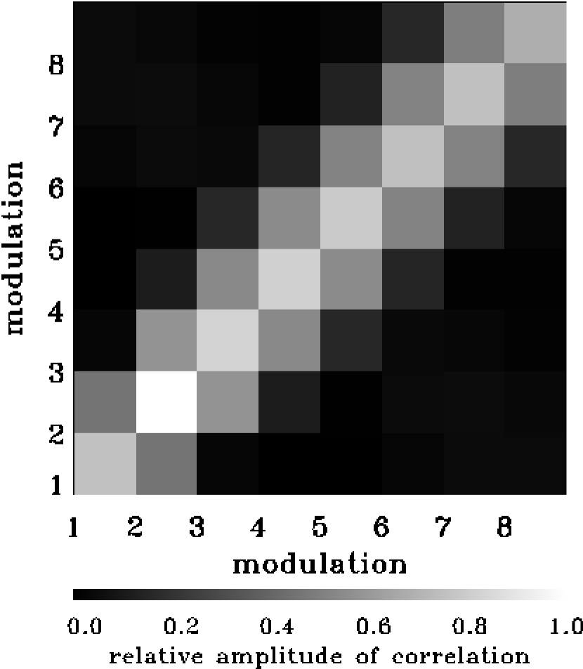
Figure 3: ${\bf C^{M}}$ for one set and feed. Elements that are more than two modulations apart are relatively uncorrelated.

With this model for the sample correlation function, it is now straightforward to compute ${\bf C^{M}}$ for each set and channel following equation (5). ${\bf C^{M}}$ matrices for channels which look at the same point on the sky and for right and left-going chopper data are averaged, yielding ${\bf C^{M}}$ matrices for both feeds in each set. As an example, ${\bf C^{M}}$ for one set and feed is shown in Figure 3.

In order to get a simple form for ${\bf C^{F}}$, the field correlation matrix, we ignore the correlations between the two feeds and assume the correlation between fields $i$ and $j$ come only from the chopper offset subtraction. We investigated several similar noise models and found that these assumptions do not change the single modulation angular power spectrum significantly, so we assume ${\bf C^{F}}$ is of this form for the cross-modulation analysis.

Finally, since this noise model is derived from sample to sample fluctuations, it is larger than the corresponding noise derived from the co-added data by a factor of $\sim 10^{4}$, so $C^{N}_{ijmm^{\prime}}$ must be normalized to the variance in the co-added data for each set. Since ${\bf C^{M}}$ accounts for the relative normalization of all of the modulations, $C^{N}_{ijmm^{\prime}}$ must be normalized to the variance in only one modulation of the co-added data for each set. We normalize to modulation 8 because we expect the higher order modulations to be least affected by the ground shield. Figure 4 shows the $\chi^{2}$/dof for each set using the final cross-modulation noise model, indicating a good final noise model.

As another check on the noise matrix used in the cross-modulation analysis, single modulation band powers were computed using the $C^{N}_{ijmm}$ components of $C^{N}_{ijmm^{\prime}}$. These are consistent with the band powers given in Coble et al. (1999).

4 MAPS

We want to estimate the power spectrum from the Python V data. Ideally, given the non-circular beam, this should be done directly from the modulated data. This would require us to form the likelihood function from the covariance matrix for the $N=5520$ data points. Inversion or Cholesky decomposition of matrices are $N^{3}$ processes so computational demands are significantly alleviated by creating a map (with $N=1666$ at highest resolution) from the modulated data and then estimating the power spectrum from the map. This technique was used in an analysis of the MSAM-I experiment (Wilson et al. 2000), for which the power spectrum estimated using the map is consistent with the power spectrum estimated directly from the modulated data. The inversion problem of map making and the circular beam assumption used in it does call for cross-checks and verification against likelihood analyses of the modulated data. The results of such tests are summarized in $\S$ 6.

The data can be expressed as:

$${\bf D}={\bf M}{\bf T}+{\bf n}$$ (7)

with noise covariance matrix $\langle nn\rangle={\bf N}={\bf C^{N}}+{\bf C^{C}}$. As mentioned above, the data vector $\bf D$ has $5520$ elements. The matrix ${\bf M}$ describes the experimental processing of the underlying temperature field; it is equal to the modulations with an index corresponding to each pixel at which we estimate the temperature $\bf T$. Given the modeling of the data as in equation (7), the minimum variance estimator for $\bf T$ is

$$\hat{T}=\tilde{\bf N}{\bf M}{\bf N^{-1}}{\bf D}.$$ (8)

This estimator will be distributed around the true temperature due to noise, where ${\bf\tilde{N}}$, the noise covariance matrix for the map, is given by

$${\bf\tilde{N}}\equiv\langle(\hat{T}-{\bf T})(\hat{T}-{\bf T})\rangle={\bf\left(M^{T}N^{-1}M\right)^{-1}}.$$ (9)

The inversion in equation (9) is singular, so it is performed via Singular Value Decomposition. It is obvious which modes are singular and should be neglected. We have tested various thresholds and found no change in the results. The pixels in the map are $30^{\prime}$ in RA which corresponds to about $20^{\prime}$ on the sky. Coarser grids gave similar results for the band powers; as we will see, there is little sensitivity to modes with $\ell>200$, so $20^{\prime}$ (a third of the beam size) is more than adequate.

Another advantage of the map basis is that the theory covariance matrix is simple to compute. In the map basis, the theory covariance matrix simplifies to

$${C^{T}_{ij}}=<T_{i}T_{j}>=\sum_{\ell}{2\ell+1\over 4\pi}P_{\ell}(\cos\theta_{ij})e^{-\ell^{2}\sigma^{2}}C_{\ell},$$ (10)

where $i$ and $j$ now refer to map pixels, $P_{\ell}$ is a Legendre polynomial, and $\theta_{ij}$ is the angular separation between points. We take $\sigma=(\sigma_{az}\sigma_{el})^{1/2}=0.425\times 0.96^{\circ}$. Taking the beam to be circular will not change the band powers significantly (see $\S$ 6). From equation (10), the window functions in the map basis only depend on the angular separation $\theta_{ij}$ and not on any of the details of the observing strategy. This is a smaller basis than that used in the analysis of the modulated data which accounts for beam non-circularity, described in $\S$ 6. Indeed, one way to think of a map is that it is the linear combination of the data for which the signal (and therefore its covariance) is nearly independent of the specific experimental observing strategy. The noise covariance for the map (eq. [9]) accounts for all of the experimental processing and the constraints.

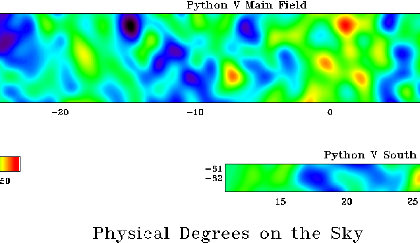
Figure 5: Wiener-filtered CMB map for the Main and South Python V regions. The maps are plotted with the same size and temperature scales. The unfiltered map was used for power spectrum estimation.

Although we are primarily interested in the map as a vehicle on the road to the power spectrum, it can also be Wiener-filtered to produce a realistic image of the sky. Wiener-filtered maps of both of the Python V regions are shown in Figure 5. We use the unfiltered map for power spectrum estimation. The map serves another useful function apart from its use for the power spectrum. One can use maps to compare different data sets that were processed in completely different manners. In $\S$ 7 we present a visual comparison of Python III and Python V. First, though, let us compute the power spectrum.

5 ANGULAR POWER SPECTRUM FROM THE MAP

We now use the map to estimate the CMB anisotropy power spectrum. Because the observations are far short of full sky coverage, we cannot determine individual $C_{\ell}$’s. Instead, we parameterize the theory covariance matrix, $\bf C^{T}$, with the power spectrum, ${\cal C}_{\ell}\equiv\ell(\ell+1)C_{\ell}/(2\pi)$, broken into bands of ${\cal C}_{\ell}$, denoted by $a$

$${\cal C}_{\ell}=\sum_{a}\chi_{{}_{a(\ell)}}{\cal C}_{a};\chi_{{}_{a(\ell)}}=\left\{\begin{array}[]{r@{\quad:\quad}l}1&\ell_{min}(a)<\ell<\ell_{max}(a)\\ 0&{\rm otherwise}\end{array}\right.$$ (11)

so that within each band $a$, ${\cal C}_{\ell}={\cal C}_{a}={\rm constant}$ and $\ell_{min}(a)$ and $\ell_{max}(a)$ delimit the range of band $a$. We use eight contiguous bands of equal width, as given in Table 2.

Since the CMB anisotropy appears to be Gaussian on the angular scales probed by the Python V experiment (Park et al. 2001; Wu et al. 2001; Shandarin et al. 2002), we can in principle use the theory covariance matrix for the map (eq. [10]) together with the map noise matrix, $\tilde{N}$, and the pixelized map data, $\bf T$, to form the full likelihood function:

$${\cal{L}}={(2\pi)^{-N/2}}{{\rm det}({\bf C})}^{-1/2}{\rm exp}{(-\chi^{2}/2)}$$ (12)

where $\chi^{2}=\bf T^{t}{\bf C^{-1}}\bf T$ and ${\bf C}={\bf C^{T}+\tilde{N}}$. We can then find the ${\cal C}_{a}$ which maximize it by conducting a direct, grid-based search in the full eight-dimensional parameter space. In practice, this is of course unfeasible because it would require of order ten likelihood evaluations in every dimension of parameter space. The likelihood function computation requires an inversion and a determinant of a large matrix (in our finest pixelization, $1666\times 1666$), so it is certainly impractical to attempt this $10^{8}$ times.

Instead, we use the quadratic estimator (Bond, Jaffe, & Knox 1998; Tegmark 1997) to find the maximum likelihood band powers and their errors. Defining

$$A_{a,ij}\equiv\left[{\bf C^{-1}}{\partial C_{T}\over\partial{\cal C}_{a}}{\bf C^{-1}}\right]_{ij}$$ (13)

where $C$ is the full theory plus noise covariance matrix, the Fisher Matrix which describes the errors is

$$F_{ab}={1\over 2}{\rm Tr}\left[{\partial C_{T}\over\partial{\cal C}_{a}}A_{b}\right]$$ (14)

and the quadratic estimator is

$$\hat{\cal C}_{a}={\cal C}_{a}^{(0)}+{1\over 2}F^{-1}_{ab}\Big{(}\bf TA_{b}\bf T-{\rm Tr}\left[{\bf C^{-1}}{\partial C_{T}\over\partial{\cal C}_{b}}\right]\Big{)}.$$ (15)

We start from a flat spectrum (e.g. all ${\cal C}_{a}^{(0)}=1000\ \mu{\rm K}^{2}$) and iterate four times. Convergence to well within the size of the error bars is usually reached by the second iteration.

The band temperature $\Delta T_{\ell}(={\cal C}_{\ell}^{1/2})$ results of the likelihood analysis are shown in Figure 6 and given in Table 2. The $\Delta T_{\ell}$ error bars here account only for the statistical uncertainties, and in particular, do not account for the calibration or beam uncertainties. The Fisher matrix is given in Table 3. We emphasize that the values of the angular power spectrum differ from those in Coble et al. (1999) because we are including more information in this analysis: the cross-modulation correlations. Again, single modulation band powers computed using the $C^{N}_{ijmm}$ components of $C^{N}_{ijmm^{\prime}}$ are consistent with the band powers given in Coble et al. (1999).

6 Comparison of Band Temperatures from Modulated Data and Map

The map has a much smaller basis ($N=1666$ at the finest pixelization) than the modulated data ($N=5520$) and hence allows for speedier likelihood analysis. However, map making is an extra step that needs verification. In particular, the map analysis has to assume a circular beam when constructing the theory covariance matrix $\bf C^{T}$.

In the modulated data basis, the beam corresponds unambiguously to the measured beam response function. The non-circular (elliptical) Python V beam is an additional complication for $\bf C^{T}$ computations. Souradeep & Ratra (2001) develop computationally rapid methods for computing $\bf C^{T}$ for experiments with non-circular beams. The constant elevation scans of the Python V experiment allow us to exactly incorporate the effects of beam non-circularity, without recourse to any approximation.

The larger size of the modulated data basis makes the 8 band likelihood analysis described in $\S$ 5 computationally expensive. We therefore choose to compare the map basis and modulated data basis results using a simplified analysis that accounts for the cross-correlation between modulations in a limited manner. This likelihood analysis estimates the band temperatures in each of the 8 $\ell$-space bins while holding fixed the other 7 band temperatures at the central values obtained in $\S$ 5.

Table 4 compares the band temperature estimates in the map basis and the modulated data basis. The two sets of results agree to 0.5 $\sigma$. The differences become larger for higher $\ell$ bins and possibly arise from non-circular beam effects. Souradeep & Ratra (2001) show that non-circular beam effects become more important above the $\ell$ value corresponding to the inverse beamwidth.

The Python V band powers can be used in combination with the results of other experiments to test for consistency and constrain cosmological parameters. This can be done in a way that accounts for the non–Gaussianity of the band power uncertainty by using the offset log–normal form for the likelihood given in Bond, Jaffe, & Knox (2000):

$$-2\ln{\cal L}=\sum_{a,b}\left(Z_{a}^{\rm t}-Z_{a}^{\rm d}\right)M_{ab}^{Z}\left(Z_{b}^{\rm t}-Z_{b}^{\rm d}\right)$$ (16)

where

$$Z_{a}^{\rm d}\equiv\ln({\cal C}_{a}+x_{a}),$$ (17)

$$Z_{a}^{\rm t}\equiv\ln\left(\sum_{l\in a}{\cal C}_{l}/N_{l}+x_{a}\right),$$ (18)

and

$$M_{ab}^{Z}\equiv F_{ab}\left({\cal C}_{a}+x_{a}\right)\left({\cal C}_{b}+x_{b}\right).$$ (19)

Again $a,b$ denote bands. We have approximated the band–power window function as a tophat with width $N_{l}=30$.

We have fit the $x_{a}$ and ${\cal C}_{a}$ parameters of this form to our one–dimensional likelihood curves, as directly evaluated from the modulated data in Table 4. The Fisher matrix comes from the quadratic estimator applied to the maps. Table 5 gives the parameters of the offset log-normal analytic fits to the band power likelihoods.

Table 6 compares band temperatures estimated with and without the circular beam approximation, from single modulation analyses where the correlations between modulations are ignored (as in Coble et al. 1999). The last column corrects the results obtained by Coble et al. (1999) for a systematic underestimation of the error bars by a factor of $\log_{10}e$. These results also use the non-circular beam and do not use the flat-sky approximation (Souradeep & Ratra 2001). The effect of the circular beam approximation on the Python V power spectrum is minimal, but would be greater for an experiment with higher S/N.

7 COMPARISON WITH PYTHON III

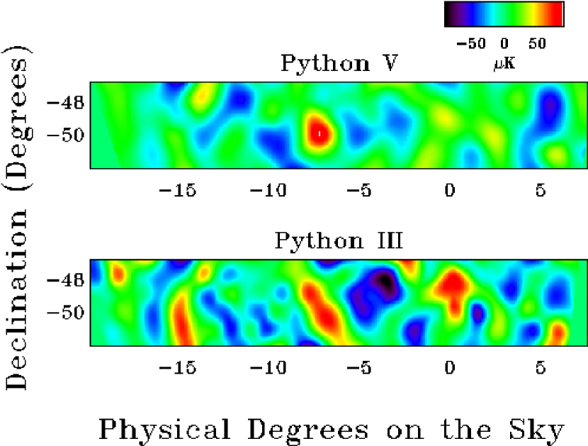
Figure 7: Comparison of Python V and Python III maps. The maps are made using only the highest S/N modes. Structures found in the Python V map are evident in the Python III map, implying that Python III and Python V are consistent with each other.

Using the technique of $\S$ 4, maps of the sky are constructed from the Python III data. We compared the maps in two different ways. First, we decomposed each map into its signal to noise eigenmodes. Keeping all the modes results in little useful visual information since most of the features in such a map are noise. Therefore, we excluded all modes with S/N less than $1.7$; stopping at S/N $=1$ retains too much noise. The resulting maps are shown in Figure 7. Since Python III has higher S/N than Python V, it retains many more modes. Therefore, not all the features seen in the Python III map should be visible in the Python V map. However, structures found in the Python V map are evident in the Python III map, implying that Python III and Python V are consistent with each other.

While the visual comparison is quite useful, it is difficult to judge the significance of the agreement in this manner. For a more quantitative comparison we use the $\beta$ test of Knox et al. (1998). This statistic has a number of possible interpretations, one of which is that it is the log of the “probability enhancement factor”. That is, it tells us how much more probable the data sets 1 and 2 are viewed jointly, as opposed to disjointly:

$$\beta\equiv\ln{P(T_{1},T_{2})\over P(T_{1})P(T_{2})}.$$ (20)

This can be re-written in terms of the likelihood function:

$$\beta=\ln{\cal L}(T_{1},T_{2})-\ln{\cal L}(T_{1})-\ln{\cal L}(T_{2})$$ (21)

The joint likelihood for the two data sets uses the likelihood equation with the data and the noise covariance being a concatenation of those from the two data sets. It also uses the theory covariance between the two sets.

We find $\beta=6.9$, which means that the data is $e^{6.9}=992$ times more probable viewed jointly than disjointly. This shows that the data sets have significantly more in common than they would if they were unrelated to each other.

We can also examine how likely this value of $\beta$ is, under these two different assumptions. The first assumption is that the data sets are related to each other exactly as we expect due to their locations on the sky, and our inference of the signal power spectrum from the Python V data. With assumption 1 we find that $\langle\beta\rangle=11.7\pm 4.3$. If instead we assume that the two data sets are completely unrelated (perhaps because one is completely contaminated), then $\langle\beta\rangle=-19.9\pm 9.4$. We see that $\beta$ differs by 1.1 standard deviations from the expected value and 2.8 standard deviations from the value expected in the absence of cross-correlations.

The $\beta$ statistic is model-dependent, but we found that it changed by less than 15% as we varied the amplitude of the assumed power spectrum by amounts consistent with the error bars and as we adjusted the calibration by $\pm 30\%$.

8 CONCLUSIONS

The Python V experiment densely samples 598 square degrees of the microwave sky and constrains the CMB anisotropy angular power spectrum from $\ell\sim$ 40 to $\ell\sim$ 260, showing that power is increasing from large to smaller ($\ell\sim$ 200) angular scales. The noise matrix constructed in $\S$ 3 enables us to simultaneously estimate the angular power spectrum in eight bands. The power spectra estimated from the map and directly from the modulated data are consistent. The rise seen in Figure 6 is characteristic of acoustic oscillations in the early Universe. A number of other measurements also indicate such a rise in power (e.g., Ganga, Ratra, & Sugiyama 1996; Netterfield et al. 1997; de Oliveira-Costa et al. 1998; Torbet et al. 1999; Podariu et al. 2001; as well as experiments mentioned in $\S$ 1). Python V extends to larger scales (lower $\ell$) than these, to the smallest scales to which COBE was sensitive.

The Python III and V experiments differ in significant ways, including frequency, receiver, year, and noise properties. Nevertheless, the maps and the $\beta$ test in $\S$ 7 indicate that they both detect similar signals, a rare and very valuable consistency check and confirmation.

Figure 1: Observing sets. Each set is observed for approximately a day (leaving $\sim$ 13 hours of good data) before moving on to the next set. Neighboring sets in the main Python V region overlap by 1 field. Circles represent the fields and arrows point to the end fields in each set. In addition to the sets shown, sets ib, jb, kb, and lb were observed with a scan pattern of 5 fields per file.

Figure 2: Correlation as a function of sample separation, $f(\Delta s)$, for all four data channels in one of the sets of files. The noise is a combination of atmospheric and instrumental noise. Channel 5 is our most sensitive channel. Channel 3 is a dark channel. These noise levels correspond to $\lesssim 1{\rm mKs}^{1/2}$.

Figure 4: $\chi^{2}$/dof for each set using the final noise matrix. Typical number of dof is 96 (= 13 stares $\times$ 8 modulations less 8 constraints), though some are much smaller. The $\chi^{2}$/dof close to 1 indicates that the final cross-modulation noise model is a good one.

Figure 6: Angular power spectrum from the cross-modulation analysis. Band powers are simultaneously estimated in 8 $\ell$-space bands. Horizontal bars indicate the width of the bands. Errors are $1\sigma$ statistical only and do not include calibration or beam uncertainties. The last two bins do not show 2$\sigma$ detections. The corresponding 2$\sigma$ upper limits on $\Delta T_{\ell}$ are 174 and 211 $\mu$K, respectively.

Term	Definition
Field	Center position for an observation.
Cycle	One back-and-forth scan along the sky centered on one
	field. Consists of 128 samples.
Stare	164 consecutive cycles, again centered on the same field.
File	Approximately 10 consecutive stares. Each stare is
	centered on a new adjacent field.
Set	Approximately 100 consecutive files (about 13 hours of
	data taking) of the same $\sim$ 10 fields.

Table 1: Data subset terminology. See Figure 1 for a visual representation of the sets of fields.

Bin	$\ell$	$\Delta T_{\ell}\ (\mu{\rm K})$
1	$44^{+15}_{-15}$	$22_{-5}^{+4}$
2	$75^{+15}_{-15}$	$24_{-7}^{+6}$
3	$106^{+15}_{-15}$	$34_{-9}^{+7}$
4	$137^{+15}_{-15}$	$50_{-12}^{+9}$
5	$168^{+15}_{-15}$	$61_{-17}^{+13}$
6	$199^{+15}_{-15}$	$77_{-28}^{+20}$
7	$230^{+15}_{-15}$	$0^{+87}_{-0}$
8	$261^{+15}_{-15}$	$69_{-69}^{+71}$

Table 2: Python V final angular power spectrum. This comes from the cross-modulation analysis. Note– Band powers are simultaneously estimated in 8 $\ell$-space bands. Error bars are 1$\sigma$ statistical only and do not account for the calibration or beam uncertainties. The last two bins do not show 2$\sigma$ detections. The corresponding 2$\sigma$ upper limits on $\Delta T_{\ell}$ are 174 and 211 $\mu$K, respectively.

	1	2	3	4	5	6	7	8
1	1.00	-0.164	0.012	-0.008	-0.003	-0.003	-0.002	-0.002
2	-0.164	1.00	-0.211	0.019	-0.011	-0.004	-0.002	-0.004
3	0.012	-0.211	1.00	-0.217	0.024	-0.012	0.000	-0.014
4	-0.008	0.019	-0.217	1.00	-0.228	0.030	0.005	-0.064
5	-0.003	-0.011	0.024	-0.228	1.00	-0.236	0.017	-0.089
6	-0.003	-0.004	-0.012	0.030	-0.236	1.00	-0.361	-0.003
7	-0.002	-0.002	0.000	0.005	0.017	-0.361	1.00	-0.385
8	-0.002	-0.004	-0.014	-0.064	-0.089	-0.003	-0.385	1.00

Table 3: Fisher Matrix $F^{-1}_{ab}/(\sqrt{F^{-1}_{aa}F^{-1}_{bb}})$.

${\rm Bin}$	$\ell$	$\Delta T_{\ell}\ (\mu{\rm K})$	$\Delta T_{\ell}\ (\mu{\rm K})$
		(Map)	(Modulated Data)
1	$44^{+15}_{-15}$	$25^{+5}_{-6}$	$25^{+6}_{-5}$
2	$75^{+15}_{-15}$	$23^{+5}_{-7}$	$22^{+6}_{-5}$
3	$106^{+15}_{-15}$	$34^{+7}_{-8}$	$32^{+8}_{-7}$
4	$137^{+15}_{-15}$	$51^{+9}_{-11}$	$50^{+9}_{-9}$
5	$168^{+15}_{-15}$	$60^{+12}_{-16}$	$56^{+15}_{-17}$
6	$199^{+15}_{-15}$	$74^{+18}_{-25}$	$67^{+22}_{-20}$
7	$230^{+15}_{-15}$	$0^{+56}_{-0}$	$9^{+53}_{-9}$
8	$261^{+15}_{-15}$	$46^{+78}_{-45}$	$70^{+39}_{-70}$

Table 4: Comparison of angular power spectra from the map and from the modulated data. Note– These are from analyses that account for the cross-correlations between modulations in a more limited manner than the full simultaneous band power estimation of Table 2, as described in the text. Error bars are 1$\sigma$ statistical only. The last two bins do not show 2$\sigma$ detections. The corresponding 2$\sigma$ upper limits on $\Delta T_{\ell}$ are 112 and 202 $\mu{\rm K}$ (from the map) and 104 and 181 $\mu{\rm K}$ (from the modulated data), respectively.

${\rm Bin}$	$x(\mu{\rm K}^{2})$	${\cal C}_{a}(\mu{\rm K}^{2})$
1	100	620
2	200	500
3	500	1050
4	5000	2600
5	5000	3150
6	6000	4570
7	20000	0
8	60000	5000

Table 5: Parameters of the offset log-normal analytic form for the band power likelihood.

Modulation	$\ell$	$\Delta T_{\ell}\ (\mu{\rm K})$	$\Delta T_{\ell}\ (\mu{\rm K})$
		(circular beam)	(elliptical beam)
1	$50^{+44}_{-29}$	$23^{+5}_{-4}$	$23^{+5}_{-4}$
2	$74^{+56}_{-39}$	$24^{+6}_{-6}$	$24^{+6}_{-6}$
3	$108^{+49}_{-41}$	$30^{+7}_{-7}$	$30^{+7}_{-7}$
4	$140^{+45}_{-41}$	$31^{+12}_{-13}$	$30^{+12}_{-13}$
5	$172^{+43}_{-40}$	$60^{+16}_{-17}$	$57^{+15}_{-16}$
6	$203^{+40}_{-38}$	$102^{+24}_{-24}$	$95^{+22}_{-22}$
7	$233^{+40}_{-38}$	$69^{+34}_{-64}$	$61^{+30}_{-57}$
8	$264^{+39}_{-37}$	$0^{+90}_{-0}$	$0^{+78}_{-0}$

Table 6: Comparison of single modulation angular power spectra with and without the circular beam approximation. Note– These are from analyses that ignore correlations between the modulations. The last column corrects the results obtained by Coble et al. (1999) for a systematic underestimation of the error bars by a factor of $\log_{10}e$. Error bars are 1$\sigma$ statistical only. The last two bins do not show 2$\sigma$ detections. The corresponding 2$\sigma$ upper limits on $\Delta T_{\ell}$ are 158 and 165 $\mu{\rm K}$ (for the circular beam) and 142 and 143 $\mu{\rm K}$ (for the elliptical beam), respectively.

References

- (1) Alvarez, D. 1996, PhD thesis, Princeton University
- (2) Bond, J. R., Jaffe, A., and Knox, L. 1998, Phys. Rev. D57, 2117
- (3) Bond, J. R., Jaffe, A., and Knox, L. 2000, ApJ, 533, 19
- (4) Coble, K. 1999, PhD thesis, University of Chicago, astro-ph/9911419
- (5) Coble, K., et al. 1999, ApJ, 519, L5
- de Oliveira-Costa et al. (1998) de Oliveira-Costa, A., Devlin, M. J., Herbig, T., Miller, A. D., Netterfield, C. B., Page, L. A., & Tegmark, M. 1998, ApJ, 509, L77
- Dragovan et al. (1994) Dragovan, M., Ruhl, J. E., Novak, G., Platt, S. R., Crone, B., Pernic, R., & Peterson, J. B. 1994 ApJ, 427, L67
- Ganga et al. (2002) Ganga, K., et al. 2002, in preparation
- Ganga, Ratra, & Sugiyama (1996) Ganga, K., Ratra, B., & Sugiyama, N. 1996, ApJ, 461, L61
- (10) Gundersen, J. O., et al. 1995, ApJ, 443, L57
- Halverson et al. (2002) Halverson, N. W., et al. 2002, ApJ, 568, 38
- (12) Knox, L., Bond, J. R., Jaffe, A. H., Segal, M., & Charbonneau, D. 1998 Phys. Rev. D, 58, 083004
- (13) Kovac, J., Dragovan, M., Schleuning, D. A., Alvarez, D., Peterson, J. B., Miller, K., Platt, S. R., Novak, G. 1997, BAAS, 29.5, 112.04
- (14) Lee, A. T., et al. 2001, ApJ, 561, L1
- Miller et al. (1999) Miller, A. D., et al. 1999, ApJ, 524, L1
- (16) Netterfield, C. B., et al. 2002, ApJ, 571, 604
- Netterfield et al. (1997) Netterfield, C. B., Devlin, M. J., Jarosik, N., Page, L., & Wollack, E. J. 1997, ApJ, 474, 47
- Park et al. (2001) Park, C.-G., Park, C., Ratra, B., & Tegmark, M. 2001, ApJ, 556, 582
- Platt et al. (1997) Platt, S. R., Kovac, J., Dragovan, M., Peterson, J. B., & Ruhl, J. E. 1997, ApJ, 475, L1
- Podariu et al. (2001) Podariu, S., Souradeep, T., Gott, J. R., Ratra, B., & Vogeley, M. S. 2001, ApJ, 559, 9
- Rocha et al. (1999) Rocha, G., Stompor, R., Ganga, K., Ratra, B., Platt, S. R., Sugiyama, N., & Górski, K. M. 1999, ApJ, 525, 1
- Ruhl et al. (1995) Ruhl, J. E., Dragovan, M., Platt, S. R., Kovac, J., & Novak, G. 1995, ApJ, 453, L1
- Shandarin et al. (2002) Shandarin, S. F., Feldman, H. A., Xu, Y., & Tegmark, M. 2002, ApJS, 141, 1
- Souradeep & Ratra (2001) Souradeep, T., & Ratra, B. 2001, ApJ, 560, 28
- (25) Tegmark, M. 1997, Phys.Rev. D, 55, 5895
- (26) Torbet, E., et al. 1999, ApJ, 521, L79
- (27) Wilson, G. W., et al. 2000, ApJ, 532, 57
- Wu et al. (2001) Wu, J.-H. P., et al. 2001, Phys. Rev. Lett., 87, 251303