Systematic Molecular Differentiation in Starless Cores
Abstract
We present evidence that low-mass starless cores, the simplest units of star formation, are systematically differentiated in their chemical composition. Molecules including CO and CS almost vanish near the core centers, where the abundance decreases by at least one or two orders of magnitude with respect to the value in the outer core. At the same time, the N2H+ molecule has a constant abundance, and the fraction of NH3 increases toward the core center. Our conclusions are based on a systematic study of 5 mostly-round starless cores (L1498, L1495, L1400K, L1517B, and L1544), which we have mapped in C18O(1–0), CS(2–1), N2H+(1–0), NH3(1,1) and (2,2) and the 1.2 mm continuum (complemented with C17O(1–0) and C34S(2–1) data for some systems). For each core we have built a spherically symmetric model in which the density is derived from the 1.2 mm continuum, the kinetic temperature from NH3, and the abundance of each molecule is derived using a Monte Carlo radiative transfer code which simultaneously fits the shape of the central spectrum and the radial profile of integrated intensity. Regarding the cores for which we have C17O(1–0) and C34S(2–1) data, the model fits these observations automatically when the standard isotopomer ratio is assumed.
As a result of this modeling, we also find that the gas kinetic temperature in each core is constant at approximately 10 K. In agreement with previous work, we find that if the dust temperature is also constant, then the density profiles are centrally flattened, and we can model them with a single analytic expression. We also find that for each core the turbulent linewidth seems constant in the inner 0.1 pc.
The very strong abundance drop of CO and CS toward the center of each core is naturally explained by the depletion of these molecules onto dust grains at densities of 2-6 cm-3. N2H+ seems unaffected by this process up to densities of several or even cm-3, while the NH3 abundance may be enhanced by its lack of depletion and reactions triggered by the disappearance of CO from the gas phase.
With the help of the Monte Carlo modeling, we show that chemical differentiation automatically explains the discrepancy between the sizes of CS and NH3 maps, a problem which has remained unexplained for more than a decade. Our models, in addition, show that a combination of radiative transfer effects can give rise to the previously observed discrepancy in the linewidth of these two tracers. Although this discrepancy has been traditionally interpreted as resulting from a systematic increase of the turbulent linewidth with radius, our models show that it can arise in conditions of constant gas turbulence.
1 Introduction
Dense molecular cores are the basic units of star formation in nearby clouds like Taurus and Perseus, where stars like our Sun have been forming over the last few million years (e.g., Myers, 1999). The study of the physical structure and kinematics of these cores is therefore crucial for our understanding of the star formation process, and molecular lines play a role in every step of this work. They probe density and temperature through their excitation, and turbulent and systematic motions through their linewidth and Doppler shifts. For this reason, chemical anomalies in the core gas can hinder our attempt to understand core properties, as the lack of a full theory of core chemical composition has made it a standard practice to assume a homogeneous abundance for all molecular species.
The presence of chemical inhomogeneities in the star-forming material at scales of dark clouds has been known for some time, with TMC-1 and L134N being the most studied examples (e.g., Little et al., 1979; Pratap et al., 1997; Swade, 1989; Dickens et al., 2000). The large-scale abundance gradients in these clouds seem best explained with time-dependent, gas-phase chemistry, implying that different condensations have evolved with different time scales (see Langer et al. 2000 and van Dishoeck & Blake 1998 for recent reviews). At the smaller size of the dense cores, a series of recent observations has shown that in some cases, the abundance of molecules like CO and CS decreases toward the core center (L1498: Kuiper et al. 1996; Willacy et al. 1998, IC5146: Kramer et al. 1999; Bergin et al. 2001, L977: Alves et al. 1999, L1544: Caselli et al. 1999, L1689B: Jessop & Ward-Thompson 2001). These decreases in abundance have been interpreted as resulting from the depletion of molecules onto dust grains at the high densities and cold temperatures occurring in dense core interiors (e.g., Bergin & Langer 1997; Charnley 1997). It is not clear, however, whether these drops in abundance are typical of all dense cores, or they are limited to a small number of objects. To answer this question, we have carried out a systematic study of a sample of 5 starless cores by observing them in a similar manner and analyzing their emission with the same radiative transfer modeling.
2 Observations
Our core sample is listed in Table 1 and was selected by inspecting the N2H+(J=1–0) maps of Caselli et al. (2001a) and choosing cores with bright emission and nearly round contours. Our goal was to select cores that had the simplest internal structure and lacked obvious outside perturbation. In order to achieve high spatial resolution, the cores were chosen from the nearby Taurus complex (estimated distance of 140 pc, Elias 1978), with the exception of L1400K, which is at an estimated distance of 170 pc (Snell, 1981). Later mapping showed that L1400K deviates significantly from spherical symmetry, which together with its non-Taurus membership made a strong case for eliminating it from the sample. We decided however to retain this source in our sample to avoid any possible bias. As we will show below, this core presents the same chemical behavior as the others, but its elongated shape makes it the hardest and most uncertain to model.
The starless classification of the cores in our sample is based on the analysis by Benson & Myers (1989), who found that they are not associated with IRAS or NIR sources. Unlike Benson & Myers (1989), however, we consider L1495 to be starless, given the large separation between this core and IRAS 04112+2803 (aka CW Tau), and the lack of apparent connection between the two. According to Myers et al. (1987), the lack of IRAS detection in a Taurus core implies a luminosity limit of L⊙ for a possible embedded source.
We observed our sample of cores in NH3 with the 100m telescope of the MPIfR in Effelsberg in 1998 October and 2001 May. The simultaneous (J,K)=(1,1) and (2,2) observations were done in frequency switching (FSW) mode with a throw of 4 MHz, and used the AK90 autocorrelator to provide a velocity resolution of 0.03 or 0.06 km s-1, depending on configuration. Cross scans on continuum point sources were used to estimate and correct pointing errors, and line observations of L1551 and S140 were used to calibrate the data, using as a reference the intensities reported by Menten & Walmsley (1985) and Ungerechts et al. (1986). The telescope beam size at the observing frequencies is approximately 40′′ (FWHM).
We observed the same 5 cores in C18O(J=1–0), CS(J=2–1), and N2H+(J=1–0) with the FCRAO111FCRAO is supported in part by the National Science Foundation under grant AST 94-20159, and is operated with permission of the Metropolitan District Commission, Commonwealth of Massachusetts. 14m telescope in 1999 November, 2000 April, and 2001 April. To obtain optically thin tracers for testing our radiative transfer models, L1498, L1517B, and L1544 were also observed in C17O(J=1–0), and L1544 was observed C34S(J=2–1). All observations were done with the SEQUOIA array receiver in FSW mode, using frequency throws of 8 MHz for N2H+(1–0), and 4 MHz for the rest of the lines. This resulted in a velocity resolution of 0.06 km s-1 for N2H+(1–0), and 0.03 km s-1 for the rest of the lines. The pointing was checked and corrected using observations of SiO masers, and the data were converted into main beam temperature scale using an efficiency of 0.55 (Ladd & Heyer, 1996). The telescope beam size at the frequencies of observation is approximately .
Finally, we observed L1498, L1495, L1400K, and L1517B in the 1.2mm continuum with the IRAM 30m telescope in 1999 December. The observations were done in on-the-fly mode with the MPIfR 37-channel bolometer array (Kreysa et al., 1998), using a scanning speed of s-1, a wobbler period of 0.5 s, and wobbler throws of 41′′ and 53′′. Three maps of L1495 were done and later combined, and the other sources were observed making single maps. The sky optical depth was estimated from sky dips before and after each individual map. All data were reduced using the NIC software (Broguière et al., 1996), and a global calibration factor of 15000 counts per Jy beam-1 was estimated from an observation of Uranus. The bolometer central frequency is 240 GHz and the telescope beam size is approximately .
For the analysis of the very narrow lines presented in this paper it is necessary to use an accurate set of rest frequencies. Currently available line catalogs (e.g., Pickett et al. 1998) do not always have the necessary precision, so a combination of accurate laboratory measurements and astronomical observations is still necessary. Here we use the set of frequencies recommended by Lee et al. (2001), who combine new (unpublished) laboratory determinations by C. Gottlieb with astronomical observations of the narrow-line core L1512, which is an improvement of the frequency set used by Tafalla et al. (1998). Following Lee et al. (2001), we use these frequencies: 93176.258 MHz for N2H+(JF1F=101–012), 97980.953 MHz for CS(J=2–1), 109782.172 for C18O(J=1–0), and 23694.4949 MHz for NH3(J,K=1,1).
3 Results
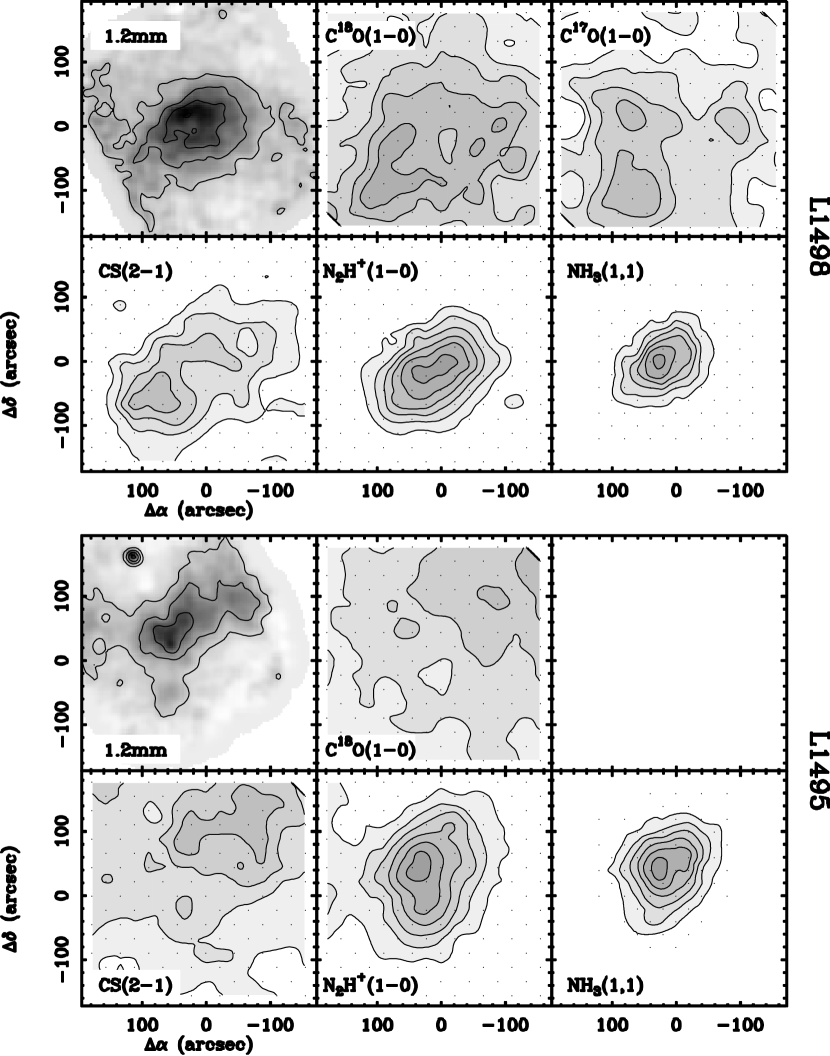
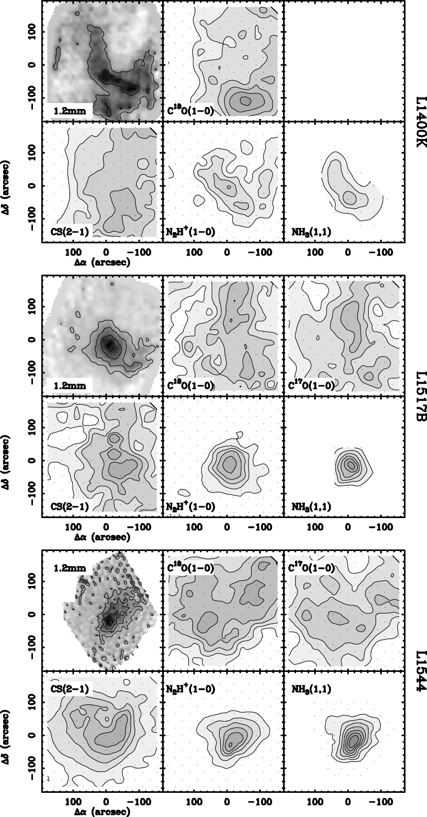
Figure 1 shows our full data set in the form of integrated intensity maps. For each starless core (L1498, L1495, L1400K, L1517B, and L1544), the three top panels display maps of what are expected to be column density tracers (dust plus the low dipole moment isotopomers C18O and C17O), and the three bottom panels display maps of high density tracers (the large dipole moment species CS, N2H+, and NH3). (The L1544 1.2mm map is from Ward-Thompson et al. 1999.) As it can be seen by simple inspection, there is a systematic pattern of emission shared by all cores. On the one hand, the continuum, N2H+, and NH3 maps are centrally concentrated, have approximately the same peak position and share very similar shapes (nearly round in L1498, L1495, and L1517B, and more elongated in L1400K and L1544). The C18O, C17O, and CS maps, on the other hand, are much more diffuse and fragmented, and have maxima which do not coincide with those of the dust, N2H+, and NH3. In fact, many maps of the CO isotopomers and CS have relative minima at the position where the other molecules peak, suggesting almost an anti correlation between the two groups of tracers.
The contrast between the centrally peaked dust emission and the fragmented C18O and C17O maps (top rows in Fig. 1) is especially striking, given that dust and C18O/C17O are both expected to trace the column density of the invisible H2 component. We can rule out a major distortion in the CO isotopomer maps due to optical depth or saturation effects, since there is excellent agreement between the C18O map and that of the rarer C17O in each core where we have observed C17O (Fig. 1). In addition, the intensity ratios between C18O and C17O are close to the expected isotopic ratio of 3.65, and a hyperfine analysis of the C17O multiplet shows a negligible optical depth (). We therefore conclude that both species are optically thin (see section 5.3 for a quantitative analysis).
Temperature gradients cannot be causing the morphological differences either, as the relative intensities of NH3(1,1) and (2,2) indicate a constant gas temperature of about 10 K in all observed sources (section 5.5). The cores moreover, being starless, lack internal heating sources to warm up the dust. Thus, we conclude that the difference between the continuum and C18O maps has arisen from spatial differences in the dust and C18O column densities. The excellent agreement between the dust emission and the emission from the high density gas tracers N2H+ and NH3 (Fig. 1) suggests that the 1.2mm continuum is a faithful tracer of the gas component, especially at the core center, and that the CO isotopomers miss the high density central region. This must be the result of a drop in CO abundance at high density, similar to that found in several starless cores by other authors (L1498: Willacy et al. 1998, IC5146: Kramer et al. 1999; Bergin et al. 2001, L977: Alves et al. 1999, L1544: Caselli et al. 1999, L1689B: Jessop & Ward-Thompson 2001)
Before estimating the abundance profile of each molecular species using a full radiative transfer analysis, we present a simple argument to estimate a lower limit to the CO abundance drop at some of the core centers. For this, we use the maps in Fig. 1, which show that the C18O and C17O emissions not only avoid the dust peak, but in most cases present a relative minimum at that position. Simple radiative transfer shows that the intensity of an optically thin, thermalized line is proportional to the molecular column density, so at a point in the map with impact parameter , the CO isotopomer emission is proportional to
where is the H2 number density, is the molecular abundance, is the length along the line of sight, and . In order to reproduce the observed C17O and C18O emission minima toward the core peaks, the amount inside the integral has to reach a relative minimum, and this can only happen if the molecular abundance decreases to more than compensate the central density peak. In other words, the observed C17O and C18O emission minima imply that the fraction of C18O and C17O decreases faster than at the core centers.
4 Core Modeling: Method Description and Density Profiles
4.1 Method Description and Justification
In the following sections we present the radiative transfer modeling needed to derive the full chemical composition of the cores. Before discussing all its details, we review here the main steps and assumptions involved in the process.
A basic simplification in our calculations is that we model the cores as spherical systems. The cores were selected from previous work (Caselli et al., 2001a) for having nearly circular contour maps. The maps of continuum, N2H+, and NH3 emission in Fig. 1 show that this is in fact the case in most systems (L1400K being the most deviant core). Although some cores would seem better modeled as spheroids, our lack of information on the line-of-sight component makes any guess about this third dimension highly uncertain. It seems, therefore, more convenient to use spherical models for the cores and to compare the predictions of those models with azimuthal averages derived from the data. This will be our approach in what follows.
The first step in our modeling is to derive density and temperature distributions for each core. We determine the density using the 1.2mm continuum emission, which seems a reliable tracer (e.g., André et al., 1996; Ward-Thompson et al., 1999) and for which we have the data of highest angular resolution. To measure the gas temperature, we have carried out a standard LTE analysis of the NH3 data and derived for each core a constant temperature of approximately 9.5 K, except for L1544 for which we derive 8.75 K. These values are in agreement with other estimates of these and similar cores (e.g., Fuller & Myers, 1993), and they will be later confirmed by our full, non LTE NH3 analysis in section 5.5.
Once densities and temperatures have been estimated, we derive molecular abundance profiles by solving the line radiative transfer with a slightly modified version of the Monte Carlo code from Bernes (1979). For each core we vary the molecular abundance of each species and the gas velocity field until the model emission (convolved with the appropriate Gaussian beam) fits both the observed radial distribution of integrated intensity and the shape of the emerging spectrum toward the core center. This approach is as close as we can get from modeling the emission at each core position with our spherical models (see, e.g., Bieging & Tafalla, 1993, for a similar procedure).
As a result of the above modeling, we derive a set of physical and chemical parameters that, for each core, simultaneously fit all the data in Fig. 1 plus the emergent central spectra. Fitting such a large number of observational data simultaneously imposes strict constrains in the model parameters, and this has made their determination a highly non linear process. Although the description in the following sections is sequential, the real fitting process required a number of iterations and back-and-forth modeling until self-consistency was achieved.
4.2 Density Profiles
We start our analysis by deriving a density distribution for each core, and we do this by modeling its dust 1.2mm emission. As our models assume spherical symmetry, we first create spherical equivalents of each core by taking azimuthal averages of the data. For the roundest cores L1517B and L1495, we simply average the data in circles, and for the more elongated L1498, L1400K, and L1544, we average the emission along ellipses with aspect ratio () and position angle () as indicated in Table 2. In these latter cases, the radial coordinate is the geometric mean of the major and minor axes of the averaging ellipse. The resulting profiles, both in linear and logarithmic scale, are presented in Figure 2.

The goal of our modeling is to find a set of density distributions whose 1.2mm dust emission fits the radial profiles shown in Fig. 2, and this requires first choosing a set of physical parameters for the dust grains. Following André et al. (1996), we use a 1.2mm emissivity cm2 g-1, although it should be noted that this parameter has an uncertainty of about a factor of 2. For dust temperature, we use a constant value equal to the gas temperature estimated from the NH3 analysis (Sec. 5.5). Recent work by Evans et al. (2001) and Zucconi et al. (2001) suggests that the dust temperature in a core may decrease toward the center due to extinction in the warming interstellar radiation field. Our NH3 data, however, suggests that the gas temperature is constant across the core (Sec. 5.5), and given that the central densities we derive ( cm-3) are high enough for gas and dust to be thermally coupled (Goldsmith & Langer, 1978; Goldsmith, 2000), we conclude that if central cooling is present, it occurs at scales smaller than the resolution of our molecular line data, so it can be safely ignored in our models.
If the dust kinetic temperature and the dust emissivity are constant, the emitted flux density from the core at the bolometer central frequency (240 GHz) is simply given by
where is the telescope beam solid angle, is the mean molecular mass, is the H2 column density (in cm-2 in the lower equation), is the FWHM of the beam in arcsec, and is the Planck function at the dust temperature . With this equation, finding the core density law becomes simplified to finding the function that gives rise to the appropriate profile. Unfortunately, the process is complicated by the need to take into account the beam smoothing and spatial filtering introduced by the on-the-fly bolometer observation. This problem, discussed in detail by Motte & André (2001), requires that a simulation of the on-the-fly observation is carried out before comparison with the data. In our case, we have used the NIC software, which lets us simulate an on-the-fly observation of the model with the same parameters as those used during the telescope run, and reduce the simulated data the same way the real data were reduced. This guarantees that data and model are properly compared.
To find the density distributions that reproduce the observed radial profiles, we iterated the fitting procedures until reasonable convergence. Previous work has shown that single power-law density profiles do not fit the emission from starless cores, and that a central flattening is always needed to reproduce the data (Ward-Thompson et al., 1994; André et al., 1996; Bacmann et al., 2000; Alves et al., 2001). Thus, it has become a standard practice to use double power laws with the inner portion nearly flat. The discontinuous derivative of these fits, however, seems rather artificial, and it appears more likely that real cores have smoother density profiles, with the double power-law expressions being just an approximation. For this reason, we have searched for a family of analytic density profiles that combine the power-law behavior for large and the central flattening at small . After different tests, we have chosen profiles of the form
where is the central density, is the radius of the “flat” region ( is the full width at half maximum), and is the asymptotic power index. As Fig. 2 shows, this family of curves, with the values for , , and indicated in Table 2, fits each of the observed radial brightness distributions with great accuracy, and it therefore constitutes the basis of our core modeling. Values of range between about and cm-3, and their major source of uncertainty is their linear dependence on (which has a factor of 2 uncertainty). is probably the best determined parameter and ranges from 3,000 to 10,000 AU, with an uncertainty of about 1,000 AU. Finally, the parameter ranges from 2 to 4, and is probably accurate to 0.25-0.5. (Whitworth & Ward-Thompson (2001) have recently proposed a similar expression, although they require , which seems outside the range of our empirically determined values. See also Langer & Willacy (2001) for an alternative fit to the L1498 density profile.)
5 Abundance Profiles: Evidence for Chemical Differentiation
5.1 Monte Carlo Model Parameters
Once the core density profiles have been determined from the continuum emission, we derive molecular abundances for all the observed species by fitting their distribution of line intensities. We do this by solving the equations of radiative transfer with a Monte Carlo code (Bernes, 1979), and as mentioned before, we assume a gas kinetic temperature of 8.75 K for L1544 and 9.5 K for the rest of the cores (section 5.5 shows how these temperatures are required by the NH3 data).
For each core, the free parameters in our Monte Carlo models are the molecular abundances, the gas velocity field (both systematic and turbulent), and the core maximum radius (almost immaterial given the steep density profiles). The velocity field is well constrained by the need to fit simultaneously the central line shape of C18O(1–0), CS(2–1), N2H+(1–0), NH3(1,1), and NH3(2,2). In this way we find that all cores but L1544 are consistent with a constant turbulent linewidth, with a value of FWHM = 0.167 km s-1 (variable km s-1 in the Bernes 1979 Monte Carlo program). For L1544, we model the emission with a turbulent linewidth of 0.13 km s-1 at the outermost radius increasing inward as up to a value of 0.25 km s-1 (Tafalla et al. 1998 also found an inward increase of the turbulent linewidth, and recently Caselli et al. 2001c have found a similar pattern studying the linewdith in the plane of the sky). This larger value of the linewidth in L1544 probably reflects the complicated kinematics of this core, already discussed by Tafalla et al. (1998) and Caselli et al. (2001c).
Together with the turbulence velocity field, we find that some cores have systematic velocity gradients along the line of sight. These gradients are required to fit the displacement of the CS self absorptions with respect to the systemic velocity (section 5.2), and, for simplicity, we parametrize the velocity field with a linear function. The values we find for (Table 3) are consistent with the typical core velocity gradients across the line of sight measured by other authors (e.g., Goodman et al. 1993).
The maximum core radius, as mentioned before, is not a critical parameter in our modeling, because the steep density gradient of each core sets an almost natural outer edge. All cores but L1544 are well fit with a maximum core radius of ( cm at the distance of Taurus and cm for L1400K), and L1544 requires twice that value. This large radius for L1544 is needed in order to fit its very deep CS self absorption, a result already found by Tafalla et al. (1998). These authors carried out a similar Monte Carlo fitting of the CS lines in L1544, but ignored possible abundance variations with radius. The models presented in this paper supersede those in Tafalla et al. (1998).
A number of tests have been carried out to ensure that the Monte Carlo results presented here are independent of the internal program parameters. During searches for the best fits, the core was divided into 100 shells spaced logarithmically, the number of model photons was set to 2000, 40 iterations were performed, and no reference radiation field was used. Previous experience had shown that these parameters were sufficient to avoid dependence on the initial conditions and to reach a stable solution. As a further test, all best models for L1517B (one of the most regular cores) have been repeated doubling the number of shells and iterations and increasing the number of photons by an order of magnitude; no significant difference has been found between these new runs and the standard cases. We take this stability of the results as an indication that the outputs from our models are true solutions to the molecular radiative transfer problem, and are not affected by the internal details of the Monte Carlo code.
5.2 C18O and CS Abundances
C18O and CS are closed-shell linear rotors with known collisional rates, and this makes their radiative transfer the easiest to calculate among all our species. For C18O, we use the molecular constants from Lovas & Krupenie (1974) together with the rate coefficients of collisional excitation by para H2 from Flower & Launay (1985). For CS, we also use the molecular constants from Lovas & Krupenie (1974), together with the collisional coefficients for para H2 from Green & Chapman (1978). A total of 9 rotational levels are considered for each molecule, and the resulting model line intensities are convolved with a Gaussian beam to simulate the result of an observation with the FCRAO telescope (FWHM of for C18O(1–0) and for CS(2–1), according to Ladd & Heyer 1996).
Our first set of models assumes spatially constant abundances for both C18O and CS. For C18O, we assume an abundance of for all cores and for CS we use different abundances so that we approximately fit the emission at large radius () for each core. The resulting radial profiles, indicated by dashed lines in the left panels of Fig. 3, fail to reproduce the observed intensities near the core center by more than a factor of 2 and are, therefore, inconsistent with the data. A similar set of constant abundance models with an abundance low enough to fit the central emission (models not shown in Fig. 3) also clearly fails to fit the C18O and CS radial profiles, in this case by underestimating the emission at large radius.
In order to improve the fits, we have run additional models with a central abundance drop. In section 3 we have seen that the C18O abundance has to decrease faster than , so with the Monte Carlo program, we have explored different analytical expressions of increasing steepness: , an exponential form, and a central abundance hole. The results derived from these models are practicably indistinguishable due to the limited resolution of the FCRAO data (), so, for simplicity, we will only present here the results derived with the exponential abundance law:
where the free parameters and represent the low-density abundance limit and the e-folding size of the abundance drop. A more detailed discussion of the shape of the abundance profiles using higher angular resolution data and multiple transitions will be presented in a forthcoming paper (Tafalla et al., 2001).


The results from this last set of models are indicated by solid lines in Fig. 3. For C18O, all models have the same value of , following Frerking et al. (1982), and the parameter ranges from about to cm-3, depending on the core (see Table 4). For CS, different cores need slightly different values of , but most estimates are close to (Table 4). The values for CS are also of the order of a few cm-3 ( cm-3 in L1544).
As seen in Fig. 3, the exponential-law abundance models fit the observed radial profiles better than the constant abundance models, especially in the inner 100′′. For L1498 and L1517B, the fits are good at all radii, and the same could be said for L1544, but the scatter in the radial profiles makes it difficult to choose the best fit at large radius. For L1495 and L1400K, however, the fits deviate from the data, and the scatter of the radial profiles makes it impossible to find a perfect fit even if we could draw an arbitrary radial profile. The origin of these fitting problems can be understood by looking at the maps in Fig. 1, which show that, in these two cores, the C18O and CS emission is so different from that of the dust, NH3, and N2H+ that it seems to trace additional structures unrelated to the cores. These structures most likely arise from nearby lower density gas, and their modeling is outside the reach of our simple scheme, which uses the continuum emission as the basis of the core model and assumes spherical symmetry. This last assumption, in addition, has the most extreme deviation in the case of L1400K, which is clearly elongated NE-SW and has additional extensition to the west (Fig. 1). The above limitations in the L1495 and L1400K models, however, do not contradict the idea of a C18O and CS abundance decrease in these two cores. Indeed, it seems that their central abundance decrease is more severe than that shown by other cores, and it is that very fact which makes them almost invisible in C18O and CS.
An additional requirement for our models is that they also fit the central spectrum, both in integrated intensity and detailed shape. As the right panels of Fig. 3 show, this is the case for L1498, L1517B, and L1544, while there are differences between model and data in L1400K and L1495 (note that the extra wing in the L1498 C18O spectrum most likely arises from the extra red component seen in the maps of Lemme et al. 1995). As with the radial profiles, the worst fits occured in the cases of L1495 and L1400K. This probably results from the difficulty in modeling extended, non spherically-symmetric material, a situation further complicated in L1495 by the presence of gas at different velocities (see our C18O spectrum and Goodman et al. 1998 for a detailed discussion of the velocity structure in L1495). For the cores with good fits (L1498, L1517B, and L1544), the agreement between model and data is achieved by finding the appropriate combination of systematic and turbulent velocity fields, a process carried out simultaneously with the modeling of the N2H+ and NH3 emission (sections 5.4 and 5.5) because our model requires that, for each core, all lines be reproduced with a single velocity field.
The CS spectra are particularly sensitive to the systematic velocity field due to the presence of self absorptions. These features naturally arise from the combination of a drop in excitation caused by the density fall off with radius and a relatively large abundance of CS in the outer core layers. Regarding the modeling of the emission, the difference in velocity between the self absorption dip and the line center constrains any possible velocity gradient along the line of sight. Most of our cores show evidence of such gradients, which we have modeled for simplicity using linear functions with the coefficients given in Table 3. We find both inward and outward velocity fields among our sample cores, with the best examples of each case being L1498 (inward) and L1517b (outward). We note that our model for the infall case L1544 lacks a gradient along the line of sight. This occurs because our modeling process was restricted to fit only the shape of the central spectrum, which appears rather symmetric and deeply self-absorbed (see Fig. 3). As Tafalla et al. (1998) have shown, L1544 presents evidence of extended inward motions in CS when off-center positions are considered, an effect that we cannot model here because of our assumption of spherical symmetry.
To conclude our analysis of the C18O and CS emission, we will estimate the abundance contrast between the core center and the outer layers implied by our models. To do this, we define for each core the parameter as the ratio between the model abundances at (half our beam) and . This parameter, shown in Table 4, is typically of the order of for both C18O and CS, indicating abundance drops for these two molecules of two orders of magnitude in each core. Such strong abundance drops are, in fact, consistent with a case in which the cores have no C18O and CS molecules at their centers.
5.3 C17O and C34S Data
The Monte Carlo modeling takes into account optical depth and trapping effects, so the poor fit of the constant abundance models in Fig. 3 cannot be explained by a failure to take those factors into accout. Still, the C18O(1–0) lines have moderate optical depth and the CS(2–1) spectra are obviously thick and self absorbed, so it seems appropriate to test the results from the previous section using optically thin lines of C17O and C34S. Here we carry out such testing with C17O(1–0) observations of the cores with brightest C18O emission (L1498, L1517B, and L1544, see Fig. 1) and C34S(2–1) data from the most self absorbed core (L1544).
The C17O molecule has hyperfine structure, and this in principle could complicate its radiative transfer modeling. The low optical depth and dipole moment of this molecule, however, causes its level excitation to be dominated by collisions, leaving trapping and splitting effects negligible. This allows us to model the C17O radiative transfer with the Monte Carlo code as if there were no hyperfine structure, and to predict the combined intensity of the three hyperfine components. The lack of model prediction for the individual components is of little consequence, as the low signal-to-noise ratio of our C17O data makes it necessary to combine the observed components before comparing them with the model predictions (see sections 5.4 and 5.5 for model line predictions for species with hyperfine structure like N2H+ and NH3).
To test the C18O calculations from the previous section, we need to create equivalent models for the rarer C17O. As the relative abundance of C18O over C17O seems constant over the Galaxy with a well measured value of 3.65 (Penzias, 1981), the C18O abundance curves determined previously can be automatically converted into C17O abundance profiles just by dividing by 3.65. This means that our C17O Monte Carlo modeling is a zero-free-parameter calculation, as it has no internal values that can be used to improve the fitting.

The top panels of Fig. 4 present a comparison between the results of our C17O(1–0) models and the FCRAO observations. Here, once again, the dashed lines represent constant abundance models and the solid lines indicate models with an exponential abundance drop. As before, the models with constant abundance fit only the outer core emission and deviate dramatically from the observed intensity toward the center. The discrepancy between the C17O constant abundance models and data is larger than seen for C18O, due to the lower optical depth of the rarer isotope, and reaches values of up to a factor of 5 toward the core centers.
In contrast to the poor fit of the constant abundance models, a remarkable fit is obtained with the models that have an exponential abundance drop (Fig. 4). These models have the same abundance profiles as those used for C18O (Table 4), with the only difference being that the value has been divided by 3.65. The good match of these models, both at large and small radii, constitutes a further and final proof that the abundance of the CO isotopes decreases sharply and systematically at high densities in all cores of our sample.
Our modeling of the C34S(2–1) emission is also a zero-free-parameter calculation. The C32S/C34S isotopic ratio in the interstellar medium equals, to a good approximation, the Solar value of 22.7 (Lucas & Liszt, 1998), so the C34S abundance profiles are just 22.7 times smaller than the CS abundance profiles. To test the main isotope CS calculations in L1544, we now run Monte Carlo radiative transfer models for C34S(2–1) for the cases of constant abundance and exponential drop.
As Fig. 4 shows, the model with constant abundance (dashed lines) is again inconsistent with the data, as it overpredicts the central intensity by more than a factor of 3. The model with an exponential abundance drop, on the other hand, again fits the data remarkably well, predicting a radial profile of the correct intensity and shape. This confirms our conclusion that the CS abundance decreases rapidly toward the core center and shows that our Monte Carlo modeling can predict accurate abundance profiles even in a case with large optical depth and strong self absorption.
5.4 N2H+ Data
Solving the radiative transfer for N2H+ is much more complicated than for CO and CS, as the two N atoms of N2H+ make its rotational level structure split into multiple hyperfine components (7 for J=1–0, 38 for 2–1, 45 for 3–2, etc.). The large number of resulting transitions, and their possible overlap, makes the solution of the radiative transfer a formidable task, and places it outside the scope of our present analysis. In this section, we discuss how to simplify the N2H+ radiative transfer treatment, and how to derive reasonably-accurate molecular abundance profiles for all our cores.
The presence of hyperfine (hf) splitting introduces two new elements into the radiative transfer. First, the splitting allows the relative population of the hyperfine sublevels to depart from their statistical weights. This effect, which gives rise to hyperfine multiplets with “non-LTE” intensity ratios, has been observed in N2H+(1–0) toward starless cores by Caselli et al. (1995). Although well-detected, this effect involves less than 10% of the emitted 1–0 radiation (Caselli et al., 1995), so it must represent only a small perturbation in the total emerging flux. In the simplified treatment presented here, we will ignore this effect assuming that inside each rotational transition the sublevels are populated according to their statistical weights.
The second effect of the hyperfine splitting is a change in the line trapping. Because of the splitting, the photons from each rotational transition can escape more easily, and this decreases their role in excitation. This effect will only be significant if trapping dominates collisions as the main excitation mechanism, and this can only occur at very large optical depths. A simple LTE fit to the observed (1–0) multiplet (the one expected to be thickest) shows that, in our cores, the averaged optical depth of the hf components does not exceed 2 even at the core maximum, and that in most cases the lines are optically thin. This suggests that collisions dominate the excitation, and that the trapping decrease represents only a minor contribution. To further explore this point, we have run radiative transfer models using two extreme limits. In one, we completely ignore the hf splitting, so the trapping is maximum, and in the other, we artificially turn off the trapping so it has no effect on excitation. The real case will necessarily lie between these two limits, closer to one or the other depending on optical depth. As a result of this test, we find that for the conditions of our cores, both limits predict the same shape of the radial profile of integrated intensity. Thus, the shape of the N2H+ abundance curve we derive from fitting the radial profile is independent of our treatment of the hf splitting. The absolute value of the abundance, in addition, typically differs between the two cases by just 30% (80% in L1495), indicating that the effect of the treatment of the hf splitting is small, and probably comparable to the uncertainties in the collisional coefficients (see below).
Given the small effect of the hf splitting in the excitation, we can simplify the radiative transfer calculation by separating the problem in two steps: the solution of the level excitation and the prediction of the emergent spectrum. In the first step, we use the Monte Carlo code without hf splitting, and calculate the combined population of each rotational level. For the collisional rate coefficients, we use the recent set for collisions between HCO+ and para H2 from Flower (1999). As Monteiro (1984) has shown, the similar rotational constants and electronic structures of N2H+ and HCO+ imply that the two species have similar cross sections, and they do in fact have collisional rates with He which are indistinguishable (see also Green, 1975). Until a specific calculation for collisions between N2H+ and H2 exist, the use of the HCO+ rates remains the most accurate choice.
Once the combined population of the rotational levels has been derived with the Monte Carlo code, we take into account the full hf structure to integrate the equation of radiative transfer along the line of sight and predict the emergent 1–0 spectrum. We assume that the hf sublevels are populated according to their statistical weights and use the relative line frequencies from Caselli et al. (1995). This emerging spectrum is finally convolved with a Gaussian function of 52.5 arcsec FWHM, to simulate the smoothing effect of the FCRAO telescope beam.

The results of the N2H+ calculations are presented in Fig. 5, where constant abundance models are compared with FCRAO observations for each core in our sample. As Fig. 5 shows, models with constant N2H+ abundance provide satisfactory fits in most cases to both the radial profile of integrated intensity (left panels) and the central emerging spectrum (right panels), in sharp contrast to what was found for C18O and CS. Although there are small deviations between model and data in Fig. 5, they most likely result from our simplified modeling and do not represent real abundance variations across the cores. This seems to be the case in L1400K, where the bright emission at large radius (and overal larger scatter) is due to the elongated shape of this core and to the presence of an extra N2H+ component to the west (see Fig. 1). Also, our inability to fit the non-gaussian shape of the L1544 spectrum is due to the presence of two velocity components in this core (Tafalla et al., 1998; Caselli et al., 2001c), which are simply modeled here with a broader gaussian component. Taking into account these effects (and the scatter in the radial profiles), we conclude that our data are consistent with all cores having constant N2H+ abundance, which we estimate to be of the order of (see Table 5 for the value derived for each core).
Although proving that the N2H+ abundance is constant has required a full radiative transfer calculation, it is clear from Fig. 1 that the similarity between the 1.2mm continuum and the N2H+ data implies an abundance behavior of this molecule different from that of CO and CS. Caselli et al. (1999) and Bergin et al. (2001) have reached similar conclusions for the cases of L1544 and IC5146, respectively, using a simpler (standard LTE) analysis than the one presented here. The different behavior of N2H+, on the one hand, and C18O and CS, on the other, is the first element of a chemical differentiation pattern that affects all our cores, and a clear sign that the common assumption that different molecular species trace the core interior equally needs serious revision.
5.5 NH3 Data
The NH3 molecule is a symmetric top with inversion doubling and consists of ortho and para species, which coexist almost independently of each other (see, e.g., Ho & Townes 1983). The (J,K)=(1,1) and (2,2) inversion lines we have observed arise from para-NH3, so our modeling will only deal with this species.
Like N2H+, NH3 has hyperfine splitting, thus, our treatment of this effect again involves some simplifications. Fortunately, the effect of the hf splitting in NH3 is even less critical than in N2H+. On the one hand, NH3 does not present hf anomalies toward dark clouds (Stutzki et al. 1984, also our own data), so the population of the hf sublevels should be proportional to their statistical weights. On the other hand, the decrease of trapping due to the hf splitting has very little effect on the collisionally dominated NH3 excitation. This once again, can be seen by comparing models with the two extreme trapping treatments (see section 5.4), which for L1517B (the roundest and second brightest core in NH3) give rise to an abundance difference of less than 10%. As before, such a difference is a negligible factor, comparable to our calibration uncertainty.
Following our N2H+ treatment, we first solve the NH3 level populations assuming no hf splitting and then calculate the emerging spectrum using sublevel populations proportional to the statistical weights. To do this, we have modified the Monte Carlo code to include the inversion doubling of the rotational levels in a symmetric top molecule. Given the low gas temperature in our cores (9.0-9.5 K), more than 99.99% of the para-NH3 population is expected to lie in the 6 levels resulting from the inversion of the rotational states (J,K)=(1,1), (2,1), and (2,2), so only those will be considered in our models. The energies of these levels have been calculated with the parameters of Poynter & Kakar (1975), and the results have been checked against the values in Pickett et al. (1998). The 6 inversion levels are connected by 5 radiative transitions, and their Einstein coefficients are given by the standard expression for a symmetric top molecule (see, e.g., Townes & Schawlow 1955) with a dipole moment of 1.476 debye (Cohen & Poynter, 1974). Collisional coefficients connecting all levels have been calculated by Danby et al. (1988) for temperatures between 15 and 300 K, and their results show that the de-excitation coefficients depend weakly on temperature. Thus, we have used for our modeling the 15 K de-excitation coefficients with para H2, and calculated the temperature-dependent excitation rates using the condition of detailed balance for the correct temperature. As a final step in our calculation, the emergent intensities have been convolved with a Gaussian of FWHM, to simulate the result of an observation with the 100m telescope.
As mentioned before, a simple LTE analysis of the NH3 data indicates a constant temperature for all cores. With our Monte Carlo calculation we can now test this result by fitting the (1,1) line and checking whether the (2,2) line fits automatically. Given that the ratio between the intensity of these lines is very sensitive to the kinetic temperature (Walmsley & Ungerechts, 1983), any mismatch in the (2,2) model will indicate a deviation from the chosen temperature.
The fit of the C18O(1–0), CS(2–1), and N2H+(1–0) spectra in the previous sections has already constrained the turbulent and systematic velocity fields in the models, and this leaves the molecular abundance as the only free parameter in our NH3 calculation. As we did for the other species, we begin the analysis by running models with constant NH3 abundance and comparing them with the observed radial profiles. The dashed curves in Fig. 6 show that the emission from these models is too flat to reproduce the observed central increase in both the (1,1) and (2,2) transitions, suggesting that constant NH3 abundance models are inconsistent with the data (the L1400K emission can be fit with a constant abundance model, but our data are too noisy to tell).
The poor fit of the constant abundance models affects both the (1,1) and (2,2) transitions, so it cannot have resulted from a wrong choice in the gas kinetic temperature. It cannot be due either to an incorrect estimate of the excitation temperature, as the (1,1) and (2,2) lines are thermalized to a good approximation (gas densities are close to cm-3 while the critical density is cm-3). Different tests assuming constant excitation temperature or an excitation temperature as given by a two level approximation (e.g., Stutzki & Winnewisser, 1985) confirm the Monte Carlo results and show that fitting the observed radial profiles requires an enhancement of the central NH3 abundance.

To model the NH3 abundance enhancement we have tried different analytic expressions, such as power laws and exponential forms. The limited resolution of the observations () makes it possible to fit the data with different expressions, as long as the abundance increases by a factor of a few toward the center. Here we present the results of power law models shown by solid lines in Fig. 6. The values for and are given in Table 5, which shows that the abundance enhancement ranges between 3 and 12 (excluding L1400K).
The abundance enhancement models not only fit the (1,1) radial profiles, but those of (2,2) as well, and this implies a correct choice for the kinetic temperature of the gas from the LTE analysis. This is not surprising given the high degree of thermalization of the NH3 levels, which makes the LTE approximation rather accurate. Although it is still possible that our -resolution observations miss gas in the inner cores at significantly lower temperatures (Evans et al., 2001; Zucconi et al., 2001), the sharp central abundance increase, which biases the emission toward the innermost gas, suggests that this cold region has to be reduced to a radius significantly smaller than 0.015 pc ( at 140 pc).
Another satisfactory aspect of the NH3 model is the good fit to the central spectrum, in particular, to its hf structure. This can be partially seen in the right panels of Fig. 6, where the main and the first satellite components of the observed (1,1) spectra are compared with the model predictions. Given the absence of any free parameter to control the hf ratio of the model results, it is remarkable that in all cases the model predicts the correct intensity contrast between hf components, and therefore, the correct optical depth. This threefold fit of the NH3 data (radial profiles of two transitions and hf ratio) strongly suggests that the abundance increase of NH3 toward the core centers is an inescapable consequence of the observations.
6 Discussion
6.1 Molecular Depletion and Comparison with Models
The analysis of the previous sections shows that the cores in our sample share a similar pattern of chemical differentiation. All systems present a sharp, order of magnitude, central abundance drop in C18O and CS, a constant abundance of N2H+, and a central enhancement of NH3. This pattern seems independent of core properties like the gas velocity structure (inward/outward), the core size, or its exact shape, indicating that it has to arise from a robust and general chemical process.
The most natural explanation for the abundance drops of C18O and CS is the depletion of these molecules onto cold dust grains at high densities. Molecular depletion has been widely expected and sought (e.g., Mundy & McMullin, 1997), and our data add to an increasing number of observations that indicate its final detection (Kuiper et al., 1996; Willacy et al., 1998; Kramer et al., 1999; Alves et al., 1999; Caselli et al., 1999; Jessop & Ward-Thompson, 2001; Bergin et al., 2001). The systematic pattern in our sample cores shows that molecular depletion is not just limited to a few special cases, but that it characterizes the majority (or totality) of the starless core population at densities larger than a few cm-3 (Table 4).
The coexistence of strong C18O and CS depletion with a constant N2H+ abundance may appear at first surprising, and even more so, the enhancement of NH3 abundance at the density peak. A likely explanation for this behavior comes from the recent work by Bergin & Langer (1997, BL97 hereafter), who have presented a chemical model in which differential depletion arises naturally from the different binding energies of the different species (see also Charnley, 1997; Aikawa et al., 2001; Caselli et al., 2001c). According to BL97, the N2 molecule binds more weakly to grains than do CO and CS, and thus it is more easily desorbed. This difference in binding energies gives rise to a pattern of depletion in which N-rich molecular species survive in the gas phase at higher densities than do CO and CS, which disappear at densities of about cm-3. To further explore the BL97 model predictions, we have used our radiative transfer calculation to estimate emerging intensities for the cores in our sample.
BL97 have studied the chemical evolution of a gas parcel as its density increases with time following two different models, one based on theoretical work by Basu & Mouschovias (1994, BM94 hereafter), and the other based on a phenomenological (accretion) fit to the contraction history of L1498 (Kuiper et al., 1996). The main difference between these two models is that the BM94 contraction is rather slow (as it is driven by ambipolar diffusion), while in the accretion fit model the density initially increases much faster. For both models, BL97 studied the effect of two types of grain mantles (CO and H2O), but a look at their abundance predictions shows that significant CO depletion only occurs in models having dust grains with (tightly bound) H2O mantles. Thus, in the following discussion we concentrate on models with these types of grains.
To compare the BL97 predictions with our observations of real cores, we create a model core with the density distribution of one of our observed cores and an abundance distribution that matches point by point the abundances predicted by BL97. Unfortunately, the BL97 models never exceed densities larger than 3-5 cm-3, so no abundance predictions are given for the densities typical of our core centers (1-2 cm-3, Table 2). This is immaterial for CS and CO, since they are so depleted at these densities that the exact value of the abundance does not affect the radiative transfer results. However, it is critical for the N2H+ and NH3 analysis, as some BL97 models show the beginning of an N2H+ and NH3 abundance decrease at the highest densities (most likely due to depletion), and this makes any extrapolation to higher densities especially unreliable. For those molecules we have explored two possibilities: that the abundance stays constant at the highest densities (unlikely according to BL97 Figs. 2 and 3), and that the abundance drops by an order of magnitude for densities not studied by BL97 (a conservative depletion model).

Fig. 7 compares the BL97 model predictions for the L1517B core with our observations of C18O, CS, N2H+, and NH3 (a similar comparison with L1498 gives the same result). As can be seen, the BM94 contraction history (dashed lines) predicts C18O and CS intensities 5 times weaker than observed, while the accretion model predicts the correct C18O intensity and overestimates the CS emission by a factor of 3. The weaker C18O and CS emission in the BM94 model result from its slow core contraction, which makes the outer core material rather old (several Myr) and, therefore, heavily depleted of these species. The accretion model, on the other hand, predicts a younger outer core ( Myr) with much less depletion. The higher CS emission predicted by the accretion model arises from an overestimate of the undepleted CS abundance by at least an order of magnitude.
Both the BM94 and accretion models predict similar N2H+ and NH3 abundances, so Fig. 7 only presents the results for the accretion model. The higher curves in the figure are intensity predictions for the case of no depletion even at the highest densities, while the lower curves assume a moderate depletion of a factor of 10 for densities higher than those studied by BL97. As can be seen, the models with no depletion agree much better with observations, although these models are less likely according to the BL97 plots. The undepleted N2H+ model is particularly good, and it predicts the correct intensity within 25% (again, a possible decrease in trapping by hfs was neglected). The NH3 prediction, on the other hand, not only overestimates the intensity, but it does not reproduce the NH3 abundance increase observed toward the core centers (an ortho-para ratio of 2 was assumed). This is a general problem of the BL97 models, which predict slight NH3 abundance increases at late times, but they are too small to fit the NH3 enhancement inferred from our observations. A possible solution is suggested by the recent work of Nejad & Wagenblast (1999), whose models show a sharp enhancement of the NH3 abundance in the core inner 0.1 pc while the N2H+ fraction remains constant. More detailed modeling of the chemical reactions triggered by the disappearance from the gas phase of CO and other species is clearly necessary.
If we take the BL97 models at face value, the previous discussion implies that cores condense rapidly and have dust grains coated with H2O ice. These conclusions, however, depend critically on the assumed molecular binding energies, and they may change as more accurate molecular parameters are derived. A lower CO binding energy, for example, will slow down the rate of CO depletion, and this can favor the larger evolution time scales predicted by ambipolar diffusion. Grain properties, in addition, may evolve as molecules deplete. An initially H2O-coated grain may evolve (through CO depletion) into a CO-coated grain, and its depletion ability may obviously change, or as Caselli et al. (2001c) have proposed, the presence of atomic oxygen in the gas phase may maintain polar mantles in the densest parts of cores, given that a fraction of O will deplete and quickly be transformed in H2O. These and other uncertainties show that it is premature to infer core evolution properties from the observed pattern of abundances. Still, the reasonable success of the BL97 model (and those by Aikawa et al. 2001 and Caselli et al. 2001c) shows that most, or all, the chemical differentiation we have observed in starless cores very likely arises from depletion and reactions triggered by depletion.
6.2 A Solution to the NH3/CS Size Discrepancy
The systematic chemical differentiation of cores we have found, and particularly the CS abundance drop, suggests a natural explanation for the decade-old discrepancy between CS and NH3 observations (e.g., Fuller & Myers, 1987; Zhou et al., 1989; Pastor et al., 1991; Morata et al., 1997). This discrepancy arises because CS rotational transitions have larger critical densities than NH3 inversion transitions. Thus, when mapping a centrally concentrated core, one would expect the CS emission to appear more peaked and concentrated than the NH3 emission. In practice, however, CS maps are systematically more extended than NH3 maps, with ratios between CS and NH3 diameters of (Zhou et al., 1989) or (Myers et al., 1991).
Explanations for the larger extension of the CS emission have postulated the scattering of photons by the core outer gas (Fuller & Myers, 1987), CS abundance enhancement by shocks in the outer core layers (Zhou et al., 1989), or unresolved clumps (Taylor et al., 1996). However, it has not been proved that these mechanisms are truly at work, and the NH3/CS discrepancy has remained unsolved for more than a decade. In this section we explore quantitatively how molecular differentiation helps to explain the discrepancy, and for this purpose, we use our Monte Carlo model results as if they represented observed data and analyze them using standard procedures.
Our models, by construction, fit simultaneously the emission size of C18O(1–0), CS(2–1), N2H+(1–0), NH3(1,1) and NH3(2,2) for each of the 5 cores in our sample. This means that these models should naturally give rise to any difference in emission size between tracers and, therefore, they should reproduce the NH3/CS discrepancy. The advantage of reproducing the discrepancy with the models is that the internal model parameters are well known, so we can use the models as laboratories to explore how the discrepancy arises from the core physical properties. Taking advantage of our multi-line observations, we study the behavior of C18O and N2H+, in addition to CS and NH3.

To estimate the sizes of the emission in different molecules, we treat our model results as if they were real data taken with a telescope (FCRAO or 100m Effelsberg), and follow the standard procedure of measuring sizes using the half maximum radius (Zhou et al., 1989; Myers et al., 1991). For NH3, N2H+, and CS this process is easily done directly from the model radial profiles, but for C18O, some radial profiles present a slight central dip, so the peak intensity does not correspond to the value at the core center. For compatibility with the other molecules, we define as radius the distance at which the C18O intensity drops to half the value at the core center. Had we taken the C18O peak value (off center), the radius would have been larger, but only by a very small amount (e.g., 5% in L1517B).
Figure 8 shows the CS/C18O, NH3/CS, and N2H+/CS size ratios measured from our Monte Carlo models following the above procedure. As the figure shows, the CS radii are consistently smaller than the C18O radii by about 30%, and the NH3 and N2H+ radii are consistently smaller than the CS radii by a factor of 2 or more. Quantitatively, we find that , , and . (A direct estimate of these ratios from the sizes of the half maximum contours in the maps of Fig. 1 yields 0.77, 0.39, and 0.54 for , , and , respectively, in excellent agreement with the values estimated from the Monte Carlo models.)
The value of in our Monte Carlo models is in excellent agreement with the derived by Myers et al. (1991) from their sample of cores, and the value also agrees with the measured by Myers et al. (1991). This good match between the relative sizes of the Monte Carlo models and those of the general population of cores suggests that the models not only reproduce the details of our (small) core sample, but that they capture the basic properties of the general core population (both starless and with stars). In particular, the models automatically reproduce the CS/NH3 size discrepancy.
To understand how the CS/NH3 size discrepancy arises in the models (Fig. 8 central panel), we isolate the factors that cause the NH3 maps to be smaller and the CS maps to be larger, and look for the dominant one. The central NH3 abundance enhancement obviously decreases the size of the NH3 maps, and we quantify this effect by comparing the radii of the best fit with that of the constant abundance models in Fig. 6. In this way, we find that best-fit models (i.e., abundance enhanced) are about 30% smaller than constant-abundance models, which is the right trend but is not enough to explain the CS/NH3 size discrepancy. The small effect of the abundance enhancement is consistent with the fact that there is a similar size discrepancy between CS and the constant abundance N2H+ (see right panel in Fig. 8).
Two factors that increase the size of the CS maps are optical depth and chemical differentiation. We study the effect of optical depth by decreasing the CS abundance with a global factor of 22 (to simulate a thin C34S observation), and find that this only decreases the average half-maximum radius by a factor of 20%. This result is consistent with the C34S observations of L1544 (Fig. 4), which show that the rare-isotopomer map is only 25% smaller than the CS map, despite the fact that the main isotope is extremely thick and self absorbed. We, therefore, conclude that optical depth is only a minor factor in the size discrepancy.
Finally, we explore the effect of the central CS abundance drop by comparing the sizes of our best CS models with the sizes predicted by constant CS abundance models which fit the observed central intensity. These constant-abundance models are a full factor of 2 smaller than the models with abundance drop, so they have sizes more comparable to those of NH3 and N2H+. This means that the major contributor to the CS/NH3 model discrepancy is the central drop in CS abundance, which decreases the peak CS intensity by a factor of several (see Fig. 4 bottom panel), and this in turn increases the radius of the half-maximum contour by about a factor of 2.
6.3 The NH3/CS Linewidth Discrepancy and the Linewidth-Size Relation in Starless Cores

A problem commonly associated with the NH3/CS size discrepancy is the systematic difference in linewidths between these two dense gas tracers. In their comparison between NH3 and CS observations of dense cores, Zhou et al. (1989) found that , which is too large to be explained by optical-depth broadening of the CS lines. Given the additional larger size of the CS emission, the traditional interpretetaion of this effect has been in terms of a systematic increase in the gas turbulence with radius, following the so-called linewidth-size relation (e.g., Fuller & Myers, 1992).
Given the above explanation, it appears surprising that all our cores (but L1544) are well fit by models with constant turbulent velocity, and that for L1544, our fit requires a decrease of linewidth with radius, not an increase. This result is significant because the line modeling is very sensitive to any linewidth variation along the line of sight through the simultaneous fit of the CS(2–1) self absorption (which arises from gas at large radius) and the fit of the N2H+ and NH3 lines (which represent gas from the innermost core). The success of the constant-linewidth models suggests that, in most cores, there are no systematic variations in the turbulent-velocity field from the core center up to radii of at least 0.1 pc (core edge).
To study whether our modeling is consistent with the NH3/CS linewidth discrepancy observed in other cores, we again use our model data as if they were real observations, and measure CS and NH3 linewidths from the predicted spectra. To do this, we first convert the model spectra into CLASS format and then use that program to fit the lines. Following standard procedure, we fit the CS(2–1) lines with simple Gaussians, and the NH3(1,1) multiplets with the standard hyperfine analysis. We apply this procedure even to the obviously self-absorbed L1544 CS spectrum, and in Fig. 9 plot our model data (black squares) together with the data from Zhou et al. (1989) for starless cores (crosses). No attempt has been made to correct our model data from instrumental broadening, as the resolution of our model ensures that this effect is less than 5%.
As Fig. 9 shows, our model data lie in the same region where we find the data from observations of other cores, i.e. consistently below the line of equal NH3 and CS linewidth. This shows that our models naturally display the NH3/CS linewidth discrepancy, the way they did for the size discrepancy. The model data, in addition, predict , which is consistent with the ratio derived by Zhou et al. (1989). The clustering of most of our points in the region of smallest linewidth is probably due to the fact that we selected the most quiescent cores possible (Section 2), and in fact, all cores but L1544 were modeled using the same turbulent speed (L1544 is the outlying point with large ). From Fig. 9 and the measured linewidth ratio, we conclude that a significant NH3/CS linewidth discrepancy can be produced even in the presence of a constant turbulence velocity field, and that it does not require the presence of a systematic increase of linewidth with size.
To understand how this NH3/CS linewidth discrepancy arises in constant turbulence gas, we have analyzed how lines are generated in our models and have found two main factors that contribute to the apparent increase of the CS linewidth over that of NH3. First, there is a bias in the way the two linewidths are measured: in the standard procedure, CS linewidths are derived by fitting a single Gaussian while NH3 linewidths are estimated with a hyperfine fit. This method has the somewhat perverse effect of correcting he usually not-very-thick NH3 line for opacity broadening, while not correcting at all the always-thick CS spectra. As Zhou et al. (1989) mention, this effect contributes to, but cannot be the only factor in, the NH3/CS linewidth discrepancy.
The additional factor that enhances the CS linewidth is the presence of self absorption. Self absorption partially truncates the CS line, decreasing its peak intensity and systematically increasing the size of its half-maximum width. This effect is similar to the way the depletion of CS at the core center truncates the map of emission and increases its half-maximum radius. Together with the linewidth-measurement bias, it is responsible for the consistently larger CS linewidths in our models (systematic velocity fields have only a minor effect).
The effect of self absorption in the final linewidth is very sensitive to the velocity displacement between the emitting and absorbing gas. A large-enough displacement (like in L1498 and L1517B, see Fig. 3) produces a single-peaked line slightly broader than the NH3 line, while no displacement (like in L1544) produces a double-peaked line which yields an extremely large linewidth when fitted with a Gaussian. This effect shifts the L1544 point very far to the right in Fig. 9, and it suggests that the points with large from Zhou et al. (1989) represent spectra with deep central self-absorptions, although further work is needed to clarify this issue. (Note that the strongly double-peaked CS line from L1544 would have appeared rather diluted in the 0.09 km s-1 channels of Zhou et al. 1989, and that these authors recognize that some of their lines are truly self-absorbed.)
Our conclusion that the gas turbulence does not increase with radius in the inner part of our cores, based on the analysis of line-of-sight motions, agrees with recent studies of turbulent motions in the plane of the sky for other cores. Using NH3 as a single tracer, Barranco & Goodman (1998) find negligible linewidth variations up to distances of 0.1 pc, which is inconsistent with the factor-of-3 increase expected from the standard linewidth-size relation between 0.01 and 0.1 pc. This suggests that the common interpretation of a turbulence increase in the inner 0.1 pc of some cores, based on the combination of NH3 and CS data, may arise from the combination of optical depth effects (which increase the CS linewidth) and a central abundance drop (which increases the CS half-maximum radius).
What happens at radii larger than 0.1 pc is still unclear. Large-scale studies show that there is a true linewidth-size relation when considering whole clouds (e.g., Larson, 1981), and Goodman et al. (1998) have suggested that turbulence starts to increase at radii larger than 0.1 pc. Unfortunately their NH3 data are not sensitive enough to follow this trend very far. An alternative view suggested by some of our CS and C18O data is that the large-scale broadening may result from the overlap of different cloud fragments moving at different velocities. Further work on large-scale modeling of molecular lines should be carried out to clarify this crucial topic.
6.4 Further Consequences of Chemical Differentiation
The chemical differentiation of starless cores has additional implications for studies of low-mass star formation, and in this section we briefly discuss some aspects of this problem. CS, for example, is one of the molecules of choice for density determinations (e.g., Evans 1999), thus, its vanishing from the gas phase at densities of a few 104 cm-3 implies that any attempt to measure with this molecule the density profile of a concentrated core seems doomed to miss the inner core region and, therefore, to underestimate the central density. This same problem may affect other classical density tracers like HCO+, HCN, and H2CO (see BL97 for model predictions), and a systematic analysis is in progress for these and other molecules (Tafalla et al., in preparation). The constant abundance of N2H+ suggests that this molecule may be a robust density tracer (see Caselli et al. 1999), but its complicated hyperfine structure and a lack of accurate collisional rate coefficients make its radiative transfer much more difficult to solve. Although it may be argued that dust continuum observations may suffice to derive core density profiles (our approach in section 4.2), confirmation of these estimates with molecular observations seems necessary, given the present uncertainties in the dust emission properties.
An additional issue in the study of starless cores potentially affected by chemical differentiation is the search for infall motions. Infall searches are usually done combining observations of optically thick and thin tracers, often from different molecular species (e.g., Lee et al. 1999). A common choice consists of CS (thick) and N2H+ (thin), two species which we have shown to reside in different parts of the core. This disjoint distribution of tracers complicates the interpretation of the spectral signatures and can only be avoided using isotopomer pairs of different optical depth. The sharp central abundance drop of CS, in addition, implies that infall searches using this molecule are only sensitive to the motions of the core’s outer layers. Thus, to probe motions close to the core center, a molecular species resistant to differentiation/depletion, like N2H+, is needed. The lower optical depth of the N2H+ lines, however, complicates detecting inward motions with the standard self-absorption analysis (but see Williams et al. 1999 for a claim of N2H+ self-absorption in L1544). The search for high velocity wings in the lines of this tracer appears to be a complementary and promising technique (Bourke et al., 2001).
Chemical differentiation does not only represent an added difficulty in the study of starless cores. The time dependence of the underlying chemical processes suggests that detailed chemical modeling should allow us to reconstruct core contraction histories from observed depletion patterns. We cautioned in section 6.1 that the fast contraction scenario derived from the BL97 model is still tentative, as it depends on the exact value of the molecular binding energies, and that an accurate determination of these critical parameters is still needed to definitively test the longer time scales predicted by ambipolar diffusion models. Before such quantitative time estimates are possible, we can compare the abundance patterns in different cores in an attempt to construct a qualitative time sequence of core evolution. Most cores in our sample have similar central densities ( cm-3) and similar depletion patterns (Tables 4 and 5), so it seems likely that they are at a similar evolutionaly stage (which may be just an effect of our selection criteria). Interestingly enough, our sample contains cores with both inward and outward motions (L1498 and L1517B, respectively), suggesting that the presence of these large-scale velocity patterns has little to do with the core evolutionary state.
The only clue to an evolutionary pattern in our sample comes from the most extreme object, L1544. This core has density higher than the others by an order of magnitude ( cm-3), and its abundance pattern slightly differs in the sense that the abundance variations of CS, C18O, and NH3 occur at higher densities than in the other cores (Tables 4 and 5). This could mean that a very rapid contraction has kept frozen a chemical pattern characteristic of lower densities or that the core has contracted faster than the others, which would not allow enough time for the moderately dense gas to be chemically processed.
Clearly additional work is needed before going further with the above speculations. The chemical composition of cores with different densities and conditions should be measured in detail. Further modeling of the chemical evolution of cores as they contract is also needed. Finally, it is important to identify key molecules that allow us to distiguish between different chemical scenarios, and to characterize the chemical behavior of standard high-density tracers. The potential benefits of understanding the chemical evolution of cores make exploring these and related questions an urgent enterprise.
7 Conclusions
We have mapped 5 starless cores (L1498, L1495, L1400K, L1517B, and L1544) in C18O(1–0), CS(2–1), N2H+(1–0), NH3(1,1) and (2,2), C17O(1–0) (3 cores), C34S(2–1) (1 core), and the 1.2 mm continuum (4 cores), and complemented these data with a published 1.2mm continuum map of L1544 (Ward-Thompson et al., 1999). For each core, we have self-consistently determined the radial profile of density (from the 1.2mm continuum), temperature (from NH3), and molecular abundance (using a radiative transfer Monte Carlo model). To do this, we have fit simultaneously the central spectrum for each line and the radial profile of integrated intensity. As a result of this work, we conclude the following:
1. Each core is well fit with a radial density profile of the form where ranges from about to cm-3, is of the order of 3000-10000 AU, and ranges from 2 to 4. This type of profile naturally fits the central flattening and the large- power-law behavior found by previous authors.
2. All cores show evidence for a strong central drop in the abundance of C18O and CS. This drop can be fitted with a negative exponential dependence on density (), with an e-folding parameter of 2-6 cm-3. C17O(1–0) and C34S(2–1) observations of several cores confirm these results and show that our radiative transfer models can naturally fit this rare isotopomer emission without extra free parameters. Although limited by the resolution of our data (), we estimate that the C18O and CS central abundance drops are at least of one or two orders of magnitude in each of the cores.
3. In contrast to C18O and CS, the N2H+ abundance seems to be constant inside each core. The combination of narrow N2H+(1–0) central spectra and the presence of narrow CS(2–1) self absorptions indicate that the turbulent linewidth in each core is constant with radius.
4. The NH3(1,1) and (2,2) lines are well fit with constant temperature models of 9.5 K (8.75 K in L1544) in which the NH3 abundance increases toward the core center. The fact that the temperature is constant at densities for which gas and dust may be thermally coupled supports the assumption of constant dust temperature used in our 1.2mm continuum analysis.
5. The combination of a central C18O and CS abundance drop, a constant N2H+ abundance, and a central NH3 abundance increase seems to be a systematic characteristic of starless cores. This suggests that star-forming material is very chemically inhomogeneous before starting to collapse, and that searches for infall in starless cores should take this fact into account.
6. The pattern of chemical differentiation, especially for C18O, CS, and N2H+ is in qualitative agreement with depletion models. Quantitative agreement between the data and these models can be achieved for certain choices of their parameters, which suggest the presence of polar ices on grains and a history of core contraction more rapid than predicted by subcritical ambipolar-diffusion models. These models, however, seem to overestimate N2H+ depletion at high densities and to miss the observed central NH3 abundance increase.
7. The presence of chemical differentiation in cores automatically explains the systematic difference between map sizes of different tracers, a problem which has remained unexplained for more than a decade. Detailed Monte Carlo radiative transfer models show that CS maps, because of the central abundance decrease and radiative transfer effects, are expected to appear at least twice as large as NH3 and N2H+ maps. These latter molecules are therefore more faithful tracers of the dense core material.
8. Comparing the CS and NH3 linewidths from our Monte Carlo radiative transfer calculations, we find a systematic NH3/CS linewidth discrepancy similar to that found by other authors (e.g., Zhou et al., 1989). These linewidth discrepancies have been traditionally interpreted as resulting from a systematic increase in the turbulent linewidth with radius, but our models show that it can arise from a combination of optical depth and self absorption in the CS line. This suggests that the linewidth-size relation does not apply in the inner 0.1 pc of cores.
References
- Aikawa et al. (2001) Aikawa, Y., Ohashi, N., Inutsuka, S., Herbst, E., & Takakuwa, S. 2001, ApJ, in press
- Alves et al. (1999) Alves, J., Lada, C.J., Lada, E.A. 1999, ApJ, 515, 265
- Alves et al. (2001) Alves, J., Lada, C.J., Lada, E.A. 2001, Nat, 409, 159
- André et al. (1996) André, P., Ward-Thompson, D., & Motte, F. 1996, A&A, 314, 625
- Bacmann et al. (2000) Bacmann, A., André, P., Puget, J.-L., Abergel, A., Bontemps, S., & Ward-Thompson, D. 2000, A&A, 361, 558
- Barranco & Goodman (1998) Barranco, J.A., & Goodman, A.A. 1998, ApJ, 504, 207
- Basu & Mouschovias (1994) Basu, S., & Mouschovias, T. 1994, ApJ, 432, 720
- Bergin & Langer (1997) Bergin, E.A., & Langer, W.D. 1997, ApJ, 486, 316
- Bergin et al. (2001) Bergin, E.A., Ciardi, D.R., Lada, C.J., Alves, J., Lada, E.A. 2001, ApJ, in press
- Bernes (1979) Bernes, C. 1979, A&A, 73, 67
- Benson & Myers (1989) Benson, P.J., & Myers, P.C. 1989, ApJS, 71, 89
- Bieging & Tafalla (1993) Bieging, J.H., & Tafalla, M. 1993, AJ, 105, 576
- Bourke et al. (2001) Bourke et al. 2001, in preparation
- Broguière et al. (1996) Broguière, D., Neri, R., & Sievers, A. 1996, IRAM Tech. Report.
- Caselli et al. (1995) Caselli, P., Myers, P.C., & Thaddeus, P. 1995, ApJ, 455, L77
- Caselli et al. (1999) Caselli, P., Walmsley, C.M., Tafalla, M., Dore, L., Myers, P.C. 1999, ApJ, 523, L165
- Caselli et al. (2001a) Caselli, P., Benson, P.J., Myers, P.C., & Tafalla, M. 2001a, in preparation
- Caselli et al. (2001b) Caselli, P., Walmsley, C.M., Zucconi, A., Tafalla, M., Dore, L., & Myers, P.C. 2001b, in press
- Caselli et al. (2001c) Caselli, P., Walmsley, C.M., Zucconi, A., Tafalla, M., Dore, L., & Myers, P.C. 2001c, in press
- Charnley (1997) Charnley, S.B. 1997, MNRAS, 291, 455
- Cohen & Poynter (1974) Cohen, E.A., & Poynter, R.L. 1974, J. Mol. Spectrosc., 53, 131
- Danby et al. (1988) Danby, G., Flower, D.R., Valiron, P., Schilke, P., & Walmsley, C.M. 1988, MNRAS, 235, 229
- Dickens et al. (2000) Dickens, J.E., Irvine, W.M., Snell, R.L., Bergin, E.A., Schloerb, F.P., Pratap, P., & Miralles, M.P. 2000 ApJ, 542, 870
- Elias (1978) Elias, J.H. ApJ, 224, 857
- Evans (1999) Evans, N.J. II 1999, ARA&A, 37, 311
- Evans et al. (2001) Evans, N.J.II, Rawlings, J.M.C., Shirley, Y.L., Mundy, L.G. 2001, ApJ, in press
- Flower (1999) Flower, D.R. 1999, MNRAS, 305, 651
- Flower & Launay (1985) Flower, D.R., & Launay, J.M. 1985, MNRAS, 214, 271
- Frerking et al. (1982) Frerking, M. A., Langer, W. D., & Wilson, R. W. 1982, ApJ, 262, 590
- Fuller & Myers (1987) Fuller, G.A., & Myers, P.C. 1987, in Physical Processes in Interstellar Clouds, eds. G.E. Morfill & M. Scholer (Dordrecht: Reidel), 137
- Fuller & Myers (1992) Fuller, G.A. & Myers, P.C. 1992, ApJ, 384, 523
- Fuller & Myers (1993) Fuller, G.A., & Myers, P.C. 1993, ApJ, 418, 273
- Goldsmith (2000) Goldsmith, P.F. 2000, BAAS, 197, 1804
- Goldsmith & Langer (1978) Goldsmith, P.F., & Langer, W.D. 1978, ApJ, 222,881
- Goodman et al. (1993) Goodman, A.A., Benson, P.J., Fuller, G.A., & Myers, P.C. 1993, ApJ, 406, 528
- Goodman et al. (1998) Goodman, A.A., Barranco, J.A., Wilner, D.J., & Heyer, M.H. 1998, ApJ, 504, 223
- Green (1975) Green, S. 1975, ApJ, 201, 366
- Green & Chapman (1978) Green, S., & Chapman, S. 1978, ApJS, 37, 169
- Ho & Townes (1983) Ho, P.T.P., & Townes, C.H. 1983, ARA&A, 21, 239
- Jessop & Ward-Thompson (2001) Jessop, N.E., & Ward-Thompson, D. 2001, preprint
- Kramer et al. (1999) Kramer, C., Alves, J., Lada, C.J., Lada, E.A., Sievers, A., Ungerechts, & Walmsley, C.M. 1999, A&A, 342, 257
- Kreysa et al. (1998) Kreysa, E., et al. 1998, SPIE, 3357, 319
- Kuiper et al. (1996) Kuiper, T.B.H., Langer, W.D., & Velusamy, T. 1996, ApJ, 468, 761
- Ladd & Heyer (1996) Ladd, E. F., & Heyer, M. 1996, FCRAO Tech. Memorandum
- Langer et al. (2000) Langer, W.D., van Dishoeck, E.F., Bergin, E.A., Blake, G.A., Tielens, A.G.G.M., Velusamy, T., & Whittet, D.C.B. 2000 in Protostars and Planets IV, eds Mannings, V., Boss, A.P., Russell, S.S. (Tucson: Univ. of Arizona Press), 29
- Langer & Willacy (2001) Langer, W.D., & Willacy, K. 2001, ApJ, 557, 714
- Larson (1981) Larson, R.B. 1981, MNRAS, 194, 809
- Little et al. (1979) Little, L.T., Macdonald, G.H., Riley, P.W.,& Matheson, D.N. 1979, MNRAS, 189, 539
- Lee et al. (1999) Lee, C.W., Myers, P.C., Tafalla, M. 1999, ApJ, 526, 788
- Lee et al. (2001) Lee, C.W., Myers, P.C., Tafalla, M. 2001, ApJS, 136, 703
- Lemme et al. (1995) Lemme, C., Walmsley, C.M., Wilson, T.L., & Muders, D. 1995 A&A, 302, 509
- Lovas & Krupenie (1974) Lovas, F. J., & Krupenie, P. H. 1974, J. Phys. Chem. Ref. Data, 3, 245
- Lucas & Liszt (1998) Lucas, R., & Liszt, H. 1998, A&A, 337, 246
- Menten & Walmsley (1985) Menten, K.M., & Walmsley, C.M. 1985, A&A, 146, 369
- Monteiro (1984) Monteiro, T. 1984, MNRAS, 210, 1
- Morata et al. (1997) Morata, O., Estalella, R., López, R., & Planesas, P. 1997, MNRAS, 292, 120
- Motte & André (2001) Motte, F., & André, P. 2001, A&A, 365, 440
- Mundy & McMullin (1997) Mundy, L.G. & McMullin, J.P. 1997, in Molecules in Astrophysics: Probes and Processes, ed. E.F. van Dishoeck, (Dordrecht: Kluwer), 183
- Myers (1999) Myers, P.C. 1999, in The Physics and Chemistry of the Interstellar Medium, eds. V. Ossenkopf, J. Stutzki, and G. Winnewisser, (Herdecke: GCA-Verlag), 227
- Myers et al. (1987) Myers, P.C., Fuller, G.A., Mathieu, R.D., Beichman, C.A., Benson, P.J., Schild, R.E., & Emerson, J.P. 1987, ApJ, 319, 340
- Myers et al. (1991) Myers, P.C., Fuller, G.A., Goodman, A.A., & Benson, P.J. 1991, ApJ, 376, 561
- Nejad & Wagenblast (1999) Nejad, L.A.M., & Wagenblast, R. 1999, A&A, 350, 204
- Pastor et al. (1991) Pastor, J., Estalella, R., López, R., Anglada, G., Planesas, P., & Buj, J. 1991, A&A, 252, 320
- Penzias (1981) Penzias, A.A. 1981, ApJ, 249, 518
- Pickett et al. (1998) Pickett, H.M., Poynter, R.L., Cohen, E.A., Delitsky, M.L., Pearson, J.C., & Muller, H.S.P. 1998, J. Quant. Spectrosc. & Rad. Transfer 60, 883
- Poynter & Kakar (1975) Poynter, R.L., & Kakar, R.K. 1975, ApJS, 29, 87
- Pratap et al. (1997) Pratap, P., Dickens, J.E., Snell, R.L., Miralles, M.P., Bergin, E.A., Irvine, W.M., & Schloerb, F.P. 1997, ApJ, 486, 862
- Snell (1981) Snell, R.L. 1981, ApJS, 45, 121
- Stutzki et al. (1984) Stutzki, J., Jackson, J.M., Olberg, M., Barret, A.H., & Winnewisser, G. 1984, A&A, 139, 258
- Stutzki & Winnewisser (1985) Stutzki, J. & Winnewisser, G. 1985, A&A, 148, 254
- Swade (1989) Swade, D.A. 1989, ApJ, 345, 828
- Tafalla et al. (1998) Tafalla, M., Mardones, D., Myers, P.C. Caselli, P., Bachiller, R., & Benson, P.J. 1998, ApJ, 504, 900
- Tafalla et al. (2001) Tafalla, M. et al. 2001, in preparation
- Taylor et al. (1996) Taylor, S. D., Morata, O., Williams, D. A. 1996, A&A, 313, 269
- Townes & Schawlow (1955) Townes, C.H. & Schawlow, A.L. 1955, Microwave Spectroscopy (New York: McGraw-Hill)
- Ungerechts et al. (1986) Ungerechts, H., Winnewisser, G., & Walmsley, C.M. 1986, A&A, 157, 207
- van Dishoeck & Blake (1998) van Dishoeck, E.F., & Blake, G.A. 1998, ARA&A, 36, 317
- Walmsley & Ungerechts (1983) Walmsley, C.M., & Ungerechts, H. 1983, A&A, 122, 164
- Ward-Thompson et al. (1999) Ward-Thompson, D., Motte, F., & André, P. 1999, MNRAS, 305, 143
- Ward-Thompson et al. (1994) Ward-Thompson, D., Scott, P.F., Hills, R.E., & André, P. 1994, MNRAS, 268, 276
- Willacy et al. (1998) Willacy, K., Langer, W.D., & Velusamy, T. 1998, ApJ, 507, L171
- Williams et al. (1999) Williams, J.P., Myers, P.C., Wilner, D.J., Di Francesco, J. 1999, ApJ, 513, L61
- Whitworth & Ward-Thompson (2001) Whitworth, A.P., & Ward-Thompson, D. 2001, ApJ, 547, 317
- Zhou et al. (1989) Zhou, S., Wu, Y., Evans, N.J.II, Fuller, G.A., & Myers, P.C. 1989, ApJ, 346, 168
- Zucconi et al. (2001) Zucconi, A., Walmsley, C.M., & Galli, D. 2001, in press
| Core | ||
|---|---|---|
| L1498 | 04 07 50.0 | 25 02 13 |
| L1495 | 04 11 02.7 | 28 00 43 |
| L1400K | 04 26 51.0 | 54 45 27 |
| L1517B | 04 52 07.2 | 30 33 18 |
| L1544 | 05 01 14.0 | 25 07 00 |
| Core | Center(b)(b)Offset with respect to coordinates in Table 1. | (c)(c)Dust temperature, assumed equal to gas temperature (see text for details). | (d)(d)Aspect ratio for elliptical average. | PA(e)(e)Position angle for elliptical average. | |||
|---|---|---|---|---|---|---|---|
| (K) | (cm | ||||||
| L1498 | (0,0) | 9.5 | 0.6 | -40 | 1.0 | 75 | 4 |
| L1495 | (20,40) | 9.5 | 1.0 | 0 | 1.1 | 45 | 2 |
| L1400K | (-20,-40) | 9.5 | 0.3 | 45 | 1.2 | 30 | 2 |
| L1517B | (-10,-20) | 9.5 | 1.0 | 0 | 2.2 | 35 | 2.5 |
| L1544 | (-13,-21) | 8.75 | 0.6 | -45 | 14 | 20 | 2.5 |
| Core | VLSR | ||
|---|---|---|---|
| (km s-1) | (km s-1) | (km s-1 pc-1) | |
| L1498 | 7.80 | 0.17(a)(a)Spatially constant. | -0.47 |
| L1495 | 6.80 | 0.17(a)(a)Spatially constant. | 0.93 |
| L1400K | 3.16 | 0.17(a)(a)Spatially constant. | 1.55 |
| L1517B | 5.78 | 0.17(a)(a)Spatially constant. | 0.78 |
| L1544 | 7.20 | 0.20(b)(b)Variable, see section 5.1. | 0.00 |
| C18O | CS | |||||
|---|---|---|---|---|---|---|
| CORE | (cm-3) | (b)(b)Model abundance drop: | (cm-3) | (b)(b)Model abundance drop: | ||
| L1498 | ||||||
| L1495 | ||||||
| L1400K | ||||||
| L1517B | ||||||
| L1544 |
| N2H+ | NH3 | |||
|---|---|---|---|---|
| CORE | (a)(a)Constant N2H+ abundance. | (b)(b)NH | (b)(b)NH | (c)(c)Model abundance enhancement: . |
| L1498 | ||||
| L1495 | ||||
| L1400K | ||||
| L1517B | ||||
| L1544 |