Antiprotons from primordial black holes

Primordial black holes (pbhs) have motivated many studies since it was shown that they should evaporate and produce all kinds of particles (Hawking Hawking1 (1974)). Recent experimental measurements of cosmic rays with great accuracy, theoretical investigations on the possible formation mechanisms and detailed evaporation processes have revived the interest in such astrophysical objects. This article aims at using the latest developments on antiproton propagation models (Maurin et al. David (2001) and Donato et al. 2001a ) together with new data from BESS, CAPRICE and AMS experiments to constrain the local amount of pbh dark matter. Depending on the diffusion halo parameters and on the details of emission mechanisms, we derive an average upper limit of the order of $\rho_{\odot}^{PBH}\approx 1.7\cdot 10^{-33}$g cm^-3.

Introduction

Very small black holes could have formed in the early universe from initial density inhomogeneities (Hawking Hawking2 (1971)), from phase transition (Hawking Hawking3 (1982)), from collapse of cosmic strings (Hawking Hawking4 (1989)) or as a result of a softening of the equation of state (Canuto Canuto (1978)). It was also shown by Choptuik (Choptuik (1993)) and, more recently, studied in the framework of double inflation (Kim Kim (2000)), that pbhs could even have formed by near-critical collapse in the expanding universe.

The interest in primordial black holes was clearly revived in the last years for several reasons. First, new experimental data on gamma-rays (Connaughton Connaughton (1998)) and cosmic rays (Maki et al. Orito (1996)) together with the construction of neutrinos detectors (Bugaev & Konishchev Bugaev (2001)), of extremely high-energy particle observatories (Barrau Barrau (2000)) and of gravitational waves interferometers (Nakamura et al. Nakamura (1997)) give interesting investigation means to look for indirect signatures of pbhs. Then, primordial black holes have been used to derive a quite stringent limit on the spectral index of the initial scalar perturbation power spectrum due to a dust-like phase of the cosmological expansion (Kotok & Naselsky Kotok (1998)). It was also found that pbhs are a great probe of the early universe with a varying gravitational constant (Carr Carr2 (2001)). Finally, significant progress have been made in the understanding of the evaporation mechanism itself, both at usual energies (Parikh & Wilczek Parikh (2000)) and in the near-planckian tail of the spectrum (Barrau & Alexeyev Barrau2 (2001), Alexeyev et al. Stas (2001)).

Among other cosmic rays, antiprotons are especially interesting as their secondary flux is both rather small (the $\bar{p}/p$ ratio is lower than $10^{-4}$ at all energies) and quite well known. This study aims at deriving new estimations of the pbh local density, taking into account the latest measurements of the antiproton spectrum and realistic models for cosmic ray propagation. Contrarily to what has been thought in early studies on antiproton spectra (see, e.g., Gaisser & Schaefer Gaisser (1992) for a review) and to what is still assumed in some recent pbh studies (e.g. Kanazawa et al. Kanazawa (2000)) there is no need for any exotic astrophysical source to account for the measured $\bar{p}$ flux. On the other hand, the very good agreement between experimental data and theoretical predictions with a purely secondary origin of antiprotons (see Donato et al. 2001a ) allows to derive quite stringent upper limit on the amount of pbh dark matter. This article focuses on this point and is organised in the following way : the first section reminds general consideration on the evaporation process and on the subsequent fragmentation phenomena. The second part is devoted to the primary antiproton sources while the third part describes all propagation aspects, with a particular emphasis on the uncertainties coming from astrophysical parameters (mostly the magnetic halo thickness) and nuclear physics cross-sections. Next, the resulting “top of atmosphere” (TOA) antiproton spectra for different formation conditions and for different possible emission models are studied. Finally, we derive the resulting upper limits on the local pbh density and consider possible future developments both on the experimental and theoretical sides.

1 Antiproton emission from pbhs

1.1 Hawking process

The Hawking black hole evaporation process can be intuitively understood as a quantum creation of particles from the vacuum by an external field (see Frolov & Novikov Frolov (1998) for more details). This can occur as a result of gravitation in a region where the Killing vector is spacelike, i.e. lying inside the $\xi^{2}=0$ surface, which is the event horizon in a static spacetime. This basic argument shows that particle creation by a gravitational field, in a stationary case, is possible only if it contains a black hole. Although very similar to the effect of particle creation by an electric field, the Hawking process has a fundamental difference: since the states of negative energy are confined inside the hole, only one of the created particles can appear outside and reach infinity. This means that the classical observer has access to only a part of the total quantum system.

To derive the accurate emission process, which mimics a Planck law, Hawking used the usual quantum mechanical wave equation for a collapsing object with a postcollapse classical curved metric (Hawking Hawking5 (1975)). He found that the emission spectrum for particles of energy $Q$ per unit of time $t$ is, for each degree of freedom:

$$\frac{{\rm d}^{2}N}{{\rm d}Q{\rm d}t}=\frac{\Gamma_{s}}{h\left(\exp\left(\frac{Q}{h\kappa/4\pi^{2}c}\right)-(-1)^{2s}\right)}$$

where contributions of electric potential and angular velocity have been neglected since the black hole discharges and finishes its rotation much faster than it evaporates (Gibbons Gibbons (1975) and Page Page1 (1977)). $\kappa$ is the surface gravity, $s$ is the spin of the emitted species and $\Gamma_{s}$ is the absorption probability. If we introduce the Hawking temperature (one of the rare physics formula using all the fundamental constants) defined by

$$T=\frac{hc^{3}}{16\pi kGM}\approx\frac{10^{13}{\rm g}}{M}{\rm GeV}$$

the argument of the exponent becomes simply a function of $Q/kT$. Although the absorption probability is often approximated by its relativistic limit, we took into account in this work its real expression for non-relativistic particles:

$$\Gamma_{s}=\frac{4\pi\sigma_{s}(Q,M,\mu)}{h^{2}c^{2}}(Q^{2}-\mu^{2})$$

where $\sigma_{s}$ is the absorption cross-section computed numerically (Page Page2 (1976)) and $\mu$ is the rest mass of the emitted particle.

1.2 Hadronization

As it was shown by MacGibbon and Webber (MacGibbon1 (1990)), when the black hole temperature is greater than the quantum chromodynamics confinement scale $\Lambda_{QCD}$, quarks and gluons jets are emitted instead of composite hadrons. To evaluate the number of emitted antiprotons, one therefore needs to perform the following convolution:

$$\frac{{\rm d}^{2}N_{\bar{p}}}{{\rm d}E{\rm d}t}=\sum_{j}\int_{Q=E}^{\infty}\alpha_{j}\frac{\Gamma_{j}(Q,T)}{h}\left(e^{\frac{Q}{kT}}-(-1)^{2s_{j}}\right)^{-1}\times\frac{{\rm d}g_{j\bar{p}}(Q,E)}{{\rm d}E}{\rm d}Q$$

where $\alpha_{j}$ is the number of degrees of freedom, $E$ is the antiproton energy and ${\rm d}g_{j\bar{p}}(Q,E)/{\rm d}E$ is the normalized differential fragmentation function, i.e. the number of antiprotons between $E$ and $E+{\rm d}E$ created by a parton jet of type $j$ and energy $Q$ (including decay products). The fragmentation functions have been evaluated with the high-energy physics frequently used event generator pythia/jetset (Tjöstrand Tj (1994)), based on the so-called string fragmentation model.

2 Primary sources

In order to compute the antiproton spectrum for a given local pbh density, the number $q^{PBH}_{\bar{p}}(r,z,E)$ of antiprotons emitted with kinetic energy between $E$ and $E+{\rm d}E$ per unit volume and time, must be evaluated. It is proportional to the number ${\rm d}^{2}n/{\rm d}M{\rm d}V$, of pbhs per unit of mass and volume and to the individual flux $d^{2}N_{\bar{p}}/dE\,dt$ emitted by one pbh, so that

$$q^{prim}(r,z,E)=\int\frac{d^{2}N_{\bar{p}}(M,E)}{dE\,dt}\cdot\frac{d^{2}n(r,z)}{dM\,dV}dM$$

where $r$ and $z$ are the cylindrical coordinates describing position in our Galaxy. As the physics of evaporation and the mass spectrum of pbh do not depend on their numerical density, the primary source term can be split into a spatial and a spectral dependance, as

$$q^{prim}(r,z,E)=q^{prim}(r,z)\times Q^{PBH}(E)$$ (1)

with

$$q^{prim}(r,z)=\frac{\rho^{PBH}(r,z)}{\rho^{PBH}_{\odot}}\;\;\;\mbox{and}\;\;\;Q^{PHB}(E)=\int_{M_{min}}^{M_{max}}\frac{d^{2}N_{\bar{p}}}{dE\,dt}\cdot\frac{d^{2}n_{\odot}}{dM\,dV}dM$$ (2)

2.1 Spatial distribution

Primordial black holes should have followed the dark matter particles during the formation of halos, so that they may have the same spatial distribution. Unfortunately, this distribution is not very well known, and several independent evidences are contradictory. In the absence of a clear answer to this problem (e.g. see Ghez. et al. Ghez (1998), Gondolo & Silk Gondolo (1999), Debattista and Sellwood debattista1 (1998, 2000)), several profiles for the pbh distribution can be used, with the generic form

$$\frac{\rho^{PBH}(r,z)}{\rho_{\odot}^{PBH}}=\left(\frac{R_{\odot}}{\sqrt{r^{2}+z^{2}}}\right)^{\gamma}\left(\frac{R_{c}^{\alpha}+R_{\odot}^{\alpha}}{R_{c}^{\alpha}+(\sqrt{r^{2}+z^{2}})^{\alpha}}\right)^{\epsilon}$$ (3)

where spherical symmetry has been assumed. Different cases have been considered, with numerical values taken in Calcáneo-Roldán and Moore (calcaneo (2001)). Numerical simulations point toward singular profiles with $\gamma=1.5$, $\alpha=1.5$, $\epsilon=1$ and $R_{c}=33.2\,\mbox{kpc}$ (Moore moore (1999)) or $\gamma=1$, $\alpha=1$, $\epsilon=2$ and $R_{c}=27.7\,\mbox{kpc}$ (Navarro, Frank & White NFW (1996), hereafter NFW). We also considered an isothermal profile with $\gamma=0$, $\alpha=2$ and $\epsilon=1$ and a modified isothermal profile with $\gamma=0$, $\alpha=2$ and $\epsilon=1.5$ and $R_{c}=24.3\,\mbox{kpc}$.

2.2 Spectral dependence

It can be seen from eq. (2) that the keypoints to derive the $Q^{PHB}(E)$ term are the shape of the mass spectrum today and the boundaries of the integral. The choice of $M_{min}$ and $M_{max}$ is discussed later.

2.2.1 pbh mass spectrum

The mass spectrum today is the result of the evolution of the initial mass spectrum in time. The usual picture is based on the idea that a pbh can form if an overdense region collapses a contrast density $\delta$ (Harrison Harrison (1970), Carr & Hawking Carr3 (1974)) so that $1/3\leq\delta\leq 1$. For a scale invariant power spectrum, this leads to

$$\left(\frac{{\rm d}n}{{\rm d}M_{init}}\right)\propto M_{init}^{-5/2}.$$

This mass spectrum will be regarded as the standard model (see, e.g. Bugaev & Konishev Bugaev (2001) for a review). To deduce the mass spectrum today from this initial one, the mass loss rate must be evaluated: ${\rm d}M/{\rm d}t\approx\{7.8d_{s=1/2}+3.1d_{s=1}\}\times 10^{24}$ g³ s^-1 with $d_{s=1/2}=90$ and $d_{s=1}=27$ (MacGibbon MacGibbon3 (1991)). If we approximate the previous law with $\alpha\approx const$, which is correct as far as the number of degrees of freedom does not increase dramatically fast, the mass can be written as a function of time as:

$$M_{init}\approx(3\alpha t+M^{3})^{1/3}.$$

It is then straightforward to see that with

$$\frac{{\rm d}n}{{\rm d}M}=\frac{{\rm d}n}{{\rm d}M_{init}}\cdot\frac{{\rm d}M_{init}}{{\rm d}M}$$

the resulting spectrum today is characterised by

$$\frac{{\rm d}n}{{\rm d}M}\propto M^{2}{\rm\leavevmode\nobreak\ for\leavevmode\nobreak\ M}<M_{*}$$

$$\frac{{\rm d}n}{{\rm d}M}\propto M^{-5/2}{\rm\leavevmode\nobreak\ for\leavevmode\nobreak\ M}>M_{*}$$

where $M_{*}\approx 5\times 10^{14}{\rm g}$ is the initial mass of a pbh expiring nowadays. In this model, the mass of a pbh formed at time $t$ is determined by the horizon mass at this epoch,

$$M=\frac{1}{8}\frac{M_{Pl}}{t_{Pl}}t.$$

In the usual cosmological picture, only pbhs formed after inflation should be taken into account as those produced before would be extremely diluted due to the huge increase of the cosmic scale factor. The end-time of inflation $t_{RH}$ being related to the reheating temperature $T_{RH}$ by

$$t_{RH}\approx 0.3g^{-1/2}\frac{M_{Pl}}{T^{2}_{RH}}$$

where $g\approx 100$ is the number of degrees of freedom in the early universe, the minimal mass of pbh in the initial spectrum can be given as a function $T_{RH}$.

It should be emphasized that the shape of the spectrum below $M_{*}\approx(3\alpha t)^{1/3}$ does not depend on any assumption about the initial mass spectrum. Whatever the initial spectrum, it should increase as $M^{2}$ today: this is only due to the ${\rm d}M_{init}/{\rm d}M$ term which is proportional to $M^{2}$ for small masses whereas the ${\rm d}n/{\rm d}M_{init}$ term is nearly constant. As shown in the next section, the antiproton emission is governed by pbhs with masses below $10^{14}$g. The results derived are therefore independent of the details of the formation mechanism.

2.2.2 Cumulative source before propagation

Figure 1: Primary antiproton flux with the standard mass spectrum before propagation (in arbitrary units). Curve (1) is for $M\in[M_{Pl},10^{12}{\rm g}]$, curve (2) is for $M\in[10^{12}{\rm g},10^{13}{\rm g}]$, curve (3) is for $M\in[10^{13}{\rm g},5\cdot 10^{13}{\rm g}]$, curve (4) is for $M>5\cdot 10^{13}{\rm g}$ and the thick line is the full spectrum.

Fig. 1 gives the antiproton flux after convolution with the pbh mass spectrum before propagation. As it could be expected, pbhs heavier than $M_{*}$ nearly do not contribute as both their number density and their temperature is low. On the other hand, only pbhs with very small masses, i.e. with very high temperatures, contribute to the high energy tail of the antiproton spectrum. It should be noticed that the only reason why they do not also dominate the low energy part is that the mass spectrum behaves like $M^{2}$ below $M_{*}$. In a Friedman universe without inflation, this important feature would make the accurate choice of the mass spectrum lower bound $M_{min}$ irrelevant (as long as it remains much smaller than $M_{*}$), due to the very small number density of black holes in this mass region.

Fig. 2 shows how inflation modifies the standard mass spectrum. The reheating temperature used herafter is nothing else than a way of taking into account a cutoff in the mass spectrum due to the rather large horizon size after inflation. There is nearly no constraint, neither on the theoretical side nor on the observational one, on this reheating temperature. A reliable lower limit can only be imposed by phenomenological arguments around the nucleosynthesis values, i.e. in the MeV range (Giudice et al. Giudice (2001)). On the other hand, upper limits, taking into account the full spectrum of inflaton decay products in the thermalization process, are close to $10^{12}$ GeV (McDonald, McDonald (2000)). The main point for the antiproton emission study is that there is clearly a critical reheating temperature, $T_{RH}^{c}\approx 10^{9}$ GeV . If $T_{RH}>T_{RH}^{c}$, the standard mass spectrum today is nearly not modified by the finite horizon size after inflation, whereas if $T_{RH}<T_{RH}^{c}$, the minimal mass becomes so large that the emission is strongly reduced. It is important to notice, first, that a rather high value of $T_{RH}^{c}$ makes the existence of pbhs evaporating now into antiprotons quite unlikely, second, that the flux is varying very fast with $T_{RH}$ around $T_{RH}^{c}$.

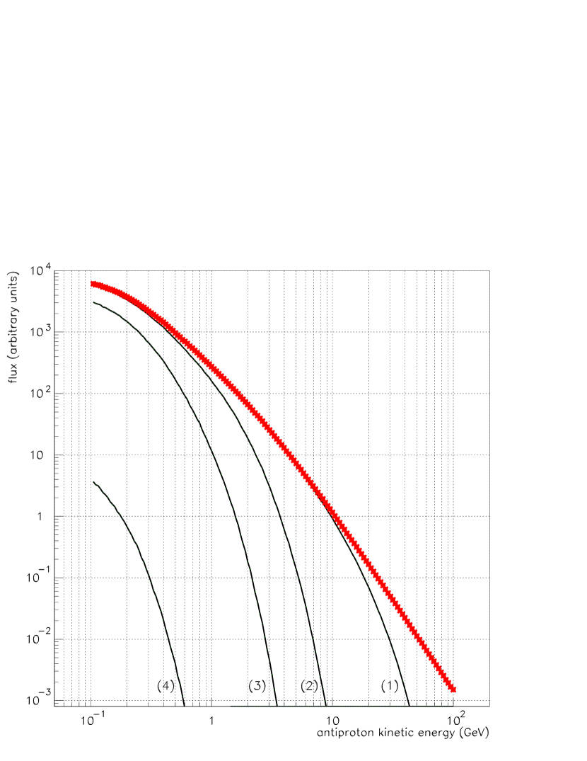
Figure 2: Primary antiproton flux with the standard mass spectrum before propagation (in arbitrary units) with different reheating temperatures. Curve (1) is for $T_{RH}=3\cdot 10^{9}$ GeV, curve (2) is for $T_{RH}=10^{9}$ GeV, curve (3) is for $T_{RH}=6\cdot 10^{8}$ GeV, curve (4) is for $T_{RH}=3\cdot 10^{8}$ GeV and the thick line is the spectrum without any cutoff.

It could also be mentioned that above some critical temperature, the emitted Hawking radiation could interact with itself and form a nearly thermal photosphere (Heckler Heckler (1997)). This idea was numerically studied (Cline et al. Cline (1999)) with the full Boltzmann equation for the particle distribution and the Hawking law as a boundary condition at horizon. For the antiproton emission, the relevant process is the formation of a quark-gluon plasma which induces energy losses before hadronization. We have taken into account this possible effect using the spectrum given by Cline et al. (Cline (1999)) : ${\rm d}^{2}N/{\rm d}E{\rm d}t\propto\exp(-E/T_{0})$ where $T_{0}\approx 300$ MeV normalized to the accurately computed Hawking spectrum. The resulting effect, dramatically reducing the evaluated flux, is shown in Fig. 3.

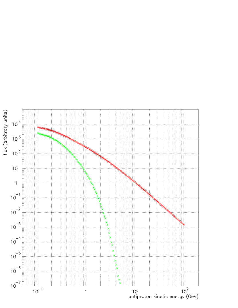
Figure 3: Primary antiproton flux with the standard mass spectrum. The higher points correspond to the pure Hawking spectrum and the lower points to the modified law with a QCD halo.

3 Propagation model

3.1 Features of the model

The propagation of cosmic rays throughout the Galaxy is described with a two–zone effective diffusion model which has been thoroughly discussed elsewhere (Maurin et al. 2001 - hereafter Paper I, Donato et al. 2001a - hereafter Paper II). We repeat here the main features of this diffusion model for the sake of completeness but we refer the reader to the above-mentioned papers for further details and justifications.

The Milky–Way is pictured as a thin gaseous disc with radius $R=20$ kpc and thickness $2h=200$ pc (see figure 4) where charged nuclei are accelerated and destroyed by collisions on the interstellar gas, yielding secondary cosmic rays. That thin ridge is sandwiched between two thick confinement layers of height $L$, called diffusion halo.

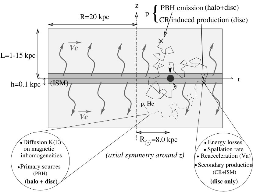
Figure 4: Schematic view of the axi-symmetric diffusion model. Secondary antiproton sources originate from cr/ism interaction in the disc only; primary sources are also distributed in the dark halo which extends far beyond the diffusion halo. In the latter case, only sources embedded in the diffusion halo contribute to the signal (see Appendix B).

The five parameters of this model are $K_{0}$, $\delta$, describing the diffusion coefficient $K(E)=K_{0}\beta{\cal R}^{-\delta}$, the halo half-height $L$, the convective velocity $V_{c}$ and the Alfven velocity $V_{a}$. Specific treatment related to $\bar{p}$ interactions (elastic scattering, inelastic destruction) and more details can also be found in Paper II.

Actually, a confident range for these five parameters has been obtained by the analysis of charged stable cosmic ray nuclei data (see Paper I). The selected parameters have been employed in Paper II to study the secondary antiproton flux, and are used again in this analysis (for specific considerations about the Alfvén velocity, see section 5.2 of Paper II). In principle, this range could be further reduced using more precise data or considering different sorts of cosmic rays. For the particular case of $\beta$ radioactive nuclei, Donato et al. 2001b showed that with existing data no definitive and strict conclusions can so far be drawn. We thus have chosen a conservative attitude and we do not apply any cut in our initial sets of parameters (which can be seen in figures 7 and 8 of Paper I).

3.2 Solution of the diffusion equation for antiprotons

Antiproton cosmic rays have been detected, and most of them were probably secondaries, i.e. they were produced by nuclear reactions of a proton or He cosmic ray (cr) nucleus impinging on interstellar (ism) hydrogen or helium atoms at rest. When energetic losses and gains are discarded, the secondary density $N^{\bar{p}}$ satisfies the relation (see Paper II for details)

$$2\,h\,\delta(z)\,q^{sec}(r,0,E) = 2\,h\,\delta(z)\,\Gamma^{ine}_{\bar{p}}\,N^{\bar{p}}(r,0,E)$$ (4)

$$+ \left\{V_{c}\frac{\partial}{\partial z}\,-\,K\left({\displaystyle\frac{\partial^{2}}{\partial z^{2}}}+\frac{1}{r}{\displaystyle\frac{\partial}{\partial r}}\left(r{\displaystyle\frac{\partial}{\partial r}}\right)\right)\right\}\,N^{\bar{p}}(r,z,E)\;\;,$$

as long as steady state holds. Due to the cylindrical geometry of the problem, it is easier to extract solutions performing Bessel expansions of all quantities over the orthogonal set of Bessel functions $J_{0}(\zeta_{i}x)$ ($\zeta_{i}$ stands for the ith zero of $J_{0}$ and $i=1\dots\infty$). The solution of equation (4) may be written as (see eqs A.3 and A.4 in paper II)

$$N^{\bar{p},\;sec}_{i}(z,E)\;=\;{\displaystyle\frac{2\,h}{A_{i}}}\;q_{i}^{sec}(E)\;\times\exp\left\{{\displaystyle\frac{V_{c}\,|z|}{2\,K}}\right\}\;\left\{{\sinh\left\{{\displaystyle\frac{S_{i}}{2}}\,\left(L-|z|\right)\right\}}\,/\,{\sinh\left\{{\displaystyle\frac{S_{i}}{2}}\,L\right\}}\right\}\;\;,$$ (5)

where the quantities $S_{i}$ and $A_{i}$ are defined as

$$S_{i}\equiv\left\{{\displaystyle\frac{V_{c}^{2}}{K^{2}}}\,+\,4{\displaystyle\frac{\zeta_{i}^{2}}{R^{2}}}\right\}^{1/2}\;\;\;\mbox{and}\;\;\;A_{i}(E)\equiv 2\,h\,\Gamma^{ine}_{\bar{p}}\;+\;V_{c}\;+\;K\,S_{i}\,{\rm coth}\left\{{\displaystyle\frac{S_{i}L}{2}}\right\}\;\;.$$ (6)

We now turn to the primary production by pbhs. It is described by a source term distributed over all the dark matter halo (see section 2.1) – this has not to be confused with the diffusion halo – whose core has a typical size of a few kpc. At $z=0$ where fluxes are measured, the corresponding density is given by (see Appendix A)

$$N^{\bar{p},prim}_{i}(0)=\exp\left(\frac{-V_{c}L}{2K}\right)\frac{y_{i}(L)}{A_{i}\sinh(S_{i}L/2)}$$ (7)

where

$$y_{i}(L)=2\int_{0}^{L}\exp\left(\frac{V_{c}}{2K}(L-z^{\prime})\right)\sinh\left(\frac{S_{i}}{2}(L-z^{\prime})\right)q^{prim}_{i}(z^{\prime})dz^{\prime}.$$ (8)

This is not the final word, as the antiproton spectrum is affected by energy losses when $\bar{p}$ interact with the galactic interstellar matter and by energy gains when reacceleration occurs. These energy changes are described by the integro–differential equation

$$A_{i}\,N^{\bar{p}}_{i}\;+\;2\,h\,\partial_{E}\left\{b^{\;\bar{p}}_{loss}(E)\,N^{\bar{p}}_{i}\,-\,K^{\;\bar{p}}_{EE}(E)\,\partial_{E}N^{\bar{p}}_{i}\right\}=2\,h\,\left\{q_{i}^{prim}(E)+q_{i}^{sec}(E)+q_{i}^{ter}(E)\right\}$$ (9)

We added a source term $q_{i}^{ter}(E)$, leading to the so-called tertiary component. It corresponds to inelastic but non-annihilating reactions of $\bar{p}$ on interstellar matter, as discussed in Paper II. The resolution of this equation proceeds as described in Appendix (A.2), (A.3) and Appendix (B) of Paper II, to which we refer for further details. The total antiproton flux is finally given by

$$N^{\bar{p},\;tot}(R_{\odot},0,E)\;=\;{\displaystyle\sum_{i=1}^{\infty}}\,\left(N^{\bar{p},\;sec}_{i}(0,E)+N^{\bar{p},\;prim}_{i}(0,E)\right)\,J_{0}\left(\zeta_{i}{\displaystyle\frac{R_{\odot}}{R}}\right)$$ (10)

where $N^{\bar{p},\;sec}_{i}(0,E)$ and $N^{\bar{p},\;prim}_{i}(0,E)$ are given by formulæ (5), (7) and (8). We emphasize that the code (and thus numerical procedures) used in this study is exactly the same as the one we used in our previous analysis (Paper I and II), with the new primary source term described above.

As previously noticed, the dark halo extends far beyond the diffusion halo whereas its core is grossly embedded within $L$. We can wonder if the external sources not comprised in the diffusive halo significantly contribute to the amount of $\bar{p}$ reaching Earth. A careful analysis shows that in the situation studied here, this contribution can be safely neglected (see Appendix B).

4 Top of atmosphere spectrum

4.1 Summary of the inputs

For the numerical results presented here, we have considered the following source term, which is a particular case of the profiles discussed in section 2.1

$$q^{prim}(r,z,E)=\rho^{PBH}_{\odot}\left(\frac{R_{c}^{2}+R_{\odot}^{2}}{R_{c}^{2}+r^{2}+z^{2}}\right)\times Q^{PBH}(E)$$ (11)

where $Q^{PBH}(E)$ was shown in figures (1), (2) and (3) for various assumptions. It corresponds to the isothermal case with a core radius $R_{c}=3$ kpc (the results are modified only by a few percents if $R_{c}$ is varied between 2 and 6 kpc). A possible flattening of this halo has been checked to be irrelevant. Actually the Moore or NFW halos do not need to be directly computed for this study as they only increase the total pbh density inside the diffusion volume for a given local density: as a result the flux is higher and the more conservative upper limit is given by the isothermal case.

The primary source term (eq. 11) is injected in eqs. (7) and (8), then added to the standard secondary contribution (eq. 5), and propagated (eq. 9) for a given set of parameters (see section 3.1). Once this interstellar flux has been calculated, it must be corrected for the effects of the solar wind, in order to be compared with the top of atmosphere observations. We have obtained the toa fluxes following the usual force field approximation (see Donato et al. Fiorenza2 (2000) and references therein). Since we will compare our predictions with data taken during a period of minimal solar activity, we have fixed the solar modulation parameter to $\phi=500$ MV.

To summarize, the whole calculation is repeated for many $Q^{PBH}(E)$ input spectra, and all possible values of the propagation parameters $V_{c}$, $L$, $K_{0}$, $V_{a}$ $\delta$ before being modulated. The modulated flux is then compared to data to give constraints on the local pbh density $\rho^{PBH}_{\odot}$.

4.2 Features of the propagated pbh spectrum

Fig. 5 shows the top of atmosphere antiproton flux resulting from the standard mass spectrum without any inflation cutoff ($T_{RH}>T_{RH}^{c}$) for a local density $\rho_{\odot}^{PBH}=10^{-32}\leavevmode\nobreak\ {\rm g}\,{\rm cm^{-3}}$. The two curves correspond to the extreme astrophysical models considered as acceptable in the extensive study of nuclei below $Z=30$ (paper I). We can notice that uncertainties due to astrophysical parameters are very important on the primary propagated $\bar{p}$ flux. The degeneracy in the diffusion parameters that one can observe for stable nuclei – and also for secondary antiprotons (see figure 7 of Paper II) – is broken down for pbh $\bar{p}$’s.

This can be easily understood: secondary $\bar{p}$ and cr nuclei are created by spallations in the galactic disc, so that all the sets of diffusion parameters that make the primaries cross the same grammage ($\sim 20$ g cm^-2) give the same secondary flux. The simplest diffusion models (no reacceleration, no galactic wind – see for example Webber et al. WebberLeeGupta (1992)) predict that the only relevant parameter is then $K_{0}/L$. On the other hand, primary antiprotons sources are located in the dark matter halo, and their flux is very sensitive to the total quantity of sources contained in the diffusion halo, i.e. to $L$. This explains the scatter of about one order of magnitude in predicted fluxes that are shown in Fig. 5 for a given local density.

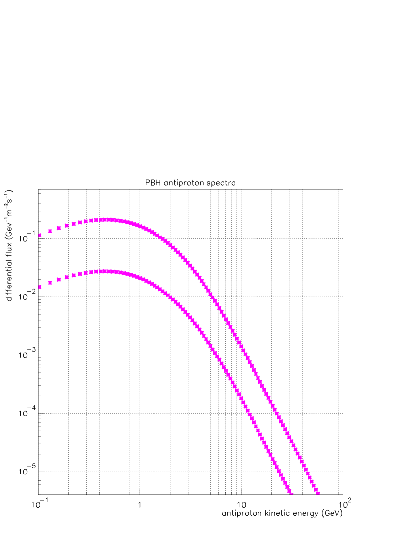
Figure 5: TOA primary antiproton flux with the standard mass spectrum after propagation for $\rho_{\odot}^{PBH}=10^{-32}\leavevmode\nobreak\ {\rm g}\,{\rm cm^{-3}}$ and extreme astrophysical models.

4.3 Comparison with previous works

In our models, all sets of parameters compatible with B/C data have been retained. In particular, a wide range of values for $L$ is allowed ($L\geq 1$ kpc) and each $L$ is correlated with the other parameters. The upper limit is set to 15 kpc, which is motivated by physical arguments (see for example Beuermann et al. Beuermann (1985) and Han et al. Han (1997) by direct observation of radio halos in galaxies, showing that $L$ is a few kpc, and Dogiel Dogiel (1991) for a compilation of evidences).

To our knowledge, the most complete studies about primary pbh antiprotons are those by Mitsui et al. (Mitsui (1996)) and Maki et al. (Orito (1996)) in which the authors use roughly adjusted values for diffusion parameters and restrict their analysis to two cases, $L=2$ kpc and $L=4$ kpc (and only one value of $K_{0}/L=0.008$ kpc Myr^-1). This is somewhat a crude estimation of what we know (or don’t know) about $L$. Moreover, in their models, neither galactic wind nor reacceleration is considered. The second point should not be very important (see Paper II) whereas the first point has a crucial impact on the detected antiproton flux. It can be shown that fluxes are at least exponentially decreased by the presence of a Galactic wind: setting $V_{c}=0$ may overestimate the number of primary $\bar{p}$ reaching Earth.

Effects of propagation parameters on primaries are qualitatively discussed in Bergström et al. (Bergstrom (1999)) for the case of susy primary antiprotons. At variance with all previous works on the subject, our treatment allows a systematic and quantitative estimation of these uncertainties, as the allowed range of propagation parameters is known from complementary cosmic ray analysis.

The difference in the spectral properties we consider are less crucial: the input pbh spectrum used here is mostly the same as in Maki et al. (Orito (1996)), whereas the accurate dimensionless absorption probability for the emitted species is taken into account instead of its high energy limit and the possible presence of a QCD halo is also investigated.

5 Upper limit on the pbh density

5.1 Method

Of course, the previously mentioned uncertainties will clearly weaken the usual upper limits on pbh density derived from antiprotons. To derive a reliable upper limit, and to account for asymmetric error bars in data, we define a generalized $\chi^{2}$ as

$$\begin{array}[]{ll}\chi^{2}=&\sum_{i}\frac{(\Phi^{th}(Q_{i})-\Phi_{i}^{exp})^{2}}{(\sigma^{exp+}_{i}+\sigma^{th+}(Q_{i}))^{2}}\Theta(\Phi^{th}(Q_{i})-\Phi^{exp}_{i})\\ &+\sum_{i}\frac{(\Phi^{th}(Q_{i})-\Phi_{i}^{exp})^{2}}{(\sigma^{exp-}_{i}+\sigma^{th-}(Q_{i}))^{2}}\Theta(\Phi^{exp}_{i}-\Phi^{th}(Q_{i})).\\ \end{array}$$

where $\sigma^{th+}$ and $\sigma^{exp+}$ ($\sigma^{th-}$ and $\sigma^{exp-}$) are the theoretical and experimental positive (negative) uncertainties. Superimposed with BESS, CAPRICE and AMS data (Orito et al. Orito1 (2000), Maeno et al. Maeno (2000), CAPRICE Coll. CAPRICE (2001), Alcaraz et al. Alcaraz (2001)), the full antiproton flux, including the secondary component and the primary component, is shown on Fig. 6 for 20 values of $\rho_{\odot}^{PBH}$ logarithmically spaced between $5\,10^{-35}$ and $10^{-32}\leavevmode\nobreak\ {\rm g}\,{\rm cm^{-3}}$. The standard mass spectrum is assumed and one astrophysical model is arbitrarily chosen, roughly corresponding to the average set of free parameters.

An upper limit on the primary flux for each value of the magnetic halo thickness is computed. The theoretical errors included in the $\chi^{2}$ function come from nuclear physics ($p+He\rightarrow\bar{p}+X$ and $He+He\rightarrow\bar{p}+X$, Paper II) and from the astrophysical parameters analysis which were added linearly, in order to remain conservative. The resulting $\chi^{2}$ leads to very conservative results as it assumes that limits on the parameters correspond to 1 sigma.

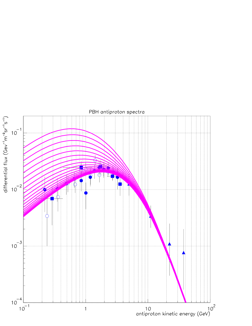
Figure 6: Experimental data from BESS95 (filled circles), BESS98 (circles), CAPRICE (triangles) and AMS (squares) superimposed with mean theoretical pbh spectra for $\rho_{\odot}^{PBH}$ between $5\cdot 10^{-35}\leavevmode\nobreak\ {\rm g}.{\rm cm}^{-3}$ (lower curve) and $10^{-32}\leavevmode\nobreak\ {\rm g}\,{\rm cm}^{-3}$ (upper curves).

5.2 Results

Fig. 7 gives the $\chi^{2}$ as a function of $\rho_{\odot}^{PBH}$ for $L=3$ kpc. The horizontal lines correspond to 63% and 99% confidence levels. In this paper the statistical significance of such numbers should be taken with care : they only refer to orders of magnitude. As expected, the $\chi^{2}$ value is constant for small pbh densities (only secondaries contribute to the flux) and is monotonically increasing without any minimum : this shows that no pbh (or any other primary source) term is needed to account for the observed antiproton flux.

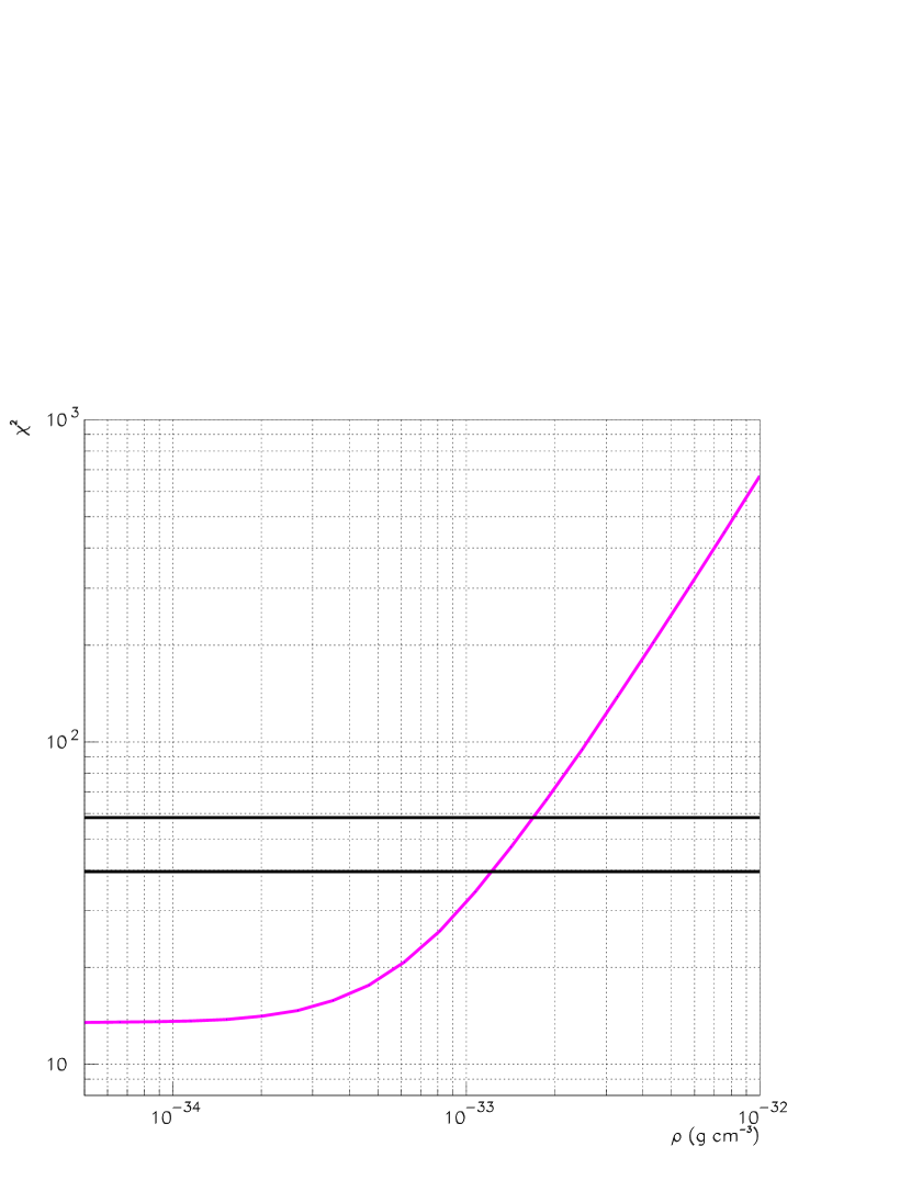
Figure 7: $\chi^{2}$ between the experimental data and the theoretical flux as a function of the local density of pbhs for a magnetic halo thickness of 3 kpc. The horizontal lines are 99% and 63% confidence levels.

Fig. 8 gives the upper limits on the local density of pbhs as a function of $L$ with the standard mass spectrum. It is a decreasing function of the halo size because a bigger diffusion region means a higher number of pbhs inside the magnetic zone for a given local density. Between $L=1$ and $L=15$ kpc (extreme astrophysical values), the 99% confidence level upper limit goes from $5.3\cdot 10^{-33}\leavevmode\nobreak\ {\rm g}\,{\rm cm}^{-3}$ to $5.1\cdot 10^{-34}\leavevmode\nobreak\ {\rm g}\,{\rm cm}^{-3}$.

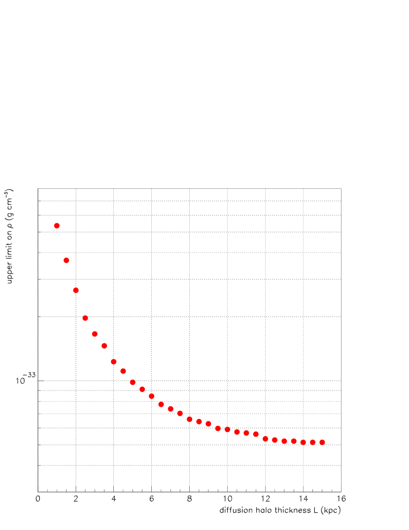
Figure 8: Upper limits on the local density of pbhs as a function of the magnetic halo thickness L.

An important point shown in section (2.2.2) is that we are sensitive only to pbhs with masses between $10^{12}$g and $10^{14}$g. The upper limit given here on the total local mass density of pbhs can therefore be given in a “safer” way as a numerical density of pbhs integrated between $10^{12}$g and $10^{14}$g. Although less interesting from the point of view of cosmology, this value has the great interest of being independent of the initial mass spectrum shape as this remains within the “increasing” part of the mass spectrum. The resulting numerical density is $n_{\odot\leavevmode\nobreak\ PBH}=3.9\cdot 10^{-51}\leavevmode\nobreak\ {\rm cm}^{-3}$ for $L=3$ kpc.

If we take into account the possible QCD photosphere (see figure 3) around pbhs, the previous upper limit is substantially weakened: $\rho_{\odot}^{PBH}<1.2\cdot 10^{-32}\leavevmode\nobreak\ {\rm g}\,{\rm cm^{-3}}$ for the ”usual” $L=3$ kpc. In this case, gamma-rays are a much more powerful tool to study pbhs. It should, nevertheless, be emphasized that this model is still controversial. First of all, because the quarks and gluons which are below threshold for pion production seem to be simply ignored, then, because the assumption that the Brehmsstrahlung interaction has a range of $1/m_{e}$ could be wrong for hard interactions, which would lead to a great overestimation of the photosphere effect (Cline, private communication).

6 Discussion and future prospects

6.1 Comparison with other existing limits

Many upper limits on the pbh explosion rate have been derived thanks to 100 MeV, 1 TeV and 100 TeV $\gamma$-rays or low-energy antiprotons.

In the ultra-high energy range, a reliable search for short gamma-ray bursts radiation from an arbitrary direction have been performed using the CYGNUS air-shower array (Alexandreas et al. Alex (1993)). No strong one second burst was observed and the resulting upper limit is $dN_{\odot exp}^{PBH}/dt\,d^{3}V\leq 0.9\cdot 10^{6}\leavevmode\nobreak\ {\rm year}^{-1}{\rm pc}^{-3}$. Very similar results were derived by the Tibet (Amenomori et al. Ame (1995)) and the AIROBIC collaborations (Funk et al. Funk (1995)). TeV gamma-rays have also been used to search for short time-scale coincidence events. The bursts detected are compatible with the expected background and the resulting upper limit obtained with 5 years of data (Connaughton Connaughton (1998)) is $dN_{\odot exp}^{PBH}/dt\,d^{3}V\leq 3\cdot 10^{6}\leavevmode\nobreak\ {\rm year}^{-1}{\rm pc}^{-3}$.

The limit coming from antiprotons has been advocated to be far better: the previous study from Maki et al. (Orito (1996)) gives $dN_{\odot exp}^{PBH}/dt\,d^{3}V\leq 2\cdot 10^{-2}\leavevmode\nobreak\ {\rm year}^{-1}{\rm pc}^{-3}$. However, we emphasize that this limit does not take into account the wide range of possible astrophysical uncertainties (in particular $L$, which can affect the limits by one order of magnitude). Moreover, we believe that the explosion rate is not the pertinent variable to use when comparing results from different approaches: thresholds differences between experiments make the meaning of ”explosion” very different. With a mass spectrum $\propto M^{2}$ for small masses, the number of exploding pbhs depends strongly on the value of the threshold. It makes the comparison of our results with the ones from Maki et al. very ambiguous. This is why we prefer to give our upper limit, either as a local mass density, assuming a standard mass spectrum, $\rho^{PBH}_{\odot}<5.3\cdot 10^{-33}\leavevmode\nobreak\ {\rm g}\,{\rm cm}^{-3}$, either as a number density, independant of the mass spectrum shape outside the relevant interval, $n_{\odot}^{PBH}<1.3\cdot 10^{-50}\leavevmode\nobreak\ {\rm cm}^{-3}$ (whatever L).

Gamma-rays in the 100 MeV region provide a sensitive probe to the presence of PBHs along the line of sight up to redshifts as large as $\sim 700$. Gamma-rays in this energy range have little interactions with the intergalactic medium and can travel on cosmological distances. The integration of the signal involves therefore a much larger scale than in the case of Milky Way antiprotons. It should also be pointed out that in this case most of the PBH population is involved as the dominant emission peaks above 100 MeV even at the present epoch. By matching the PBH cosmological emission to the extra-galactic gamma-ray diffuse background (MacGibbon & Carr MacGibbon2 (1991)), the limit $\Omega_{PBH}\leq 1.8\times 10^{-8}\,h^{-2}$ was obtained. Being mostly based on the assumption that a standard PBH mass spectrum holds above $M_{*}$, this result is robust. Our limit ($\rho^{PBH}_{\odot}<5.3\times 10^{-33}\leavevmode\nobreak\ {\rm g}\,{\rm cm}^{-3}$) also requires the same assumption. It no longer depends on the details of cosmic-ray propagation as it corresponds to the minimal possible value of 1 kpc for $L$. This result is therefore quite conservative. In order to discuss it in the light of the gamma-ray constraints, it should be noticed that any PBH population is a particular form of cold dark matter. When the latter collapses to form galactic halos and the intra-cluster medium, PBHs merely follow the collapse. Their abundance in the solar neighbourhood should trace their cosmological contribution to the overall value of $\Omega_{M}\sim 0.3-0.4$. Because a canonical isothermal halo has a solar density of $\sim 0.3$ GeV cm^-3 – $\sim 5.3\times 10^{-25}$ g cm^-3 – we infer an upper limit of $\sim 10^{-8}$ on the contribution of PBHs to the galactic – and as mentionned above to the cosmological – dark matter. Our antiproton bound translates into $\Omega_{PBH}\leq 10^{-8}\,\Omega_{M}\sim 4\times 10^{-9}$. Such a constraint is comparable to the limit derived from gamma-ray considerations. Antiprotons are produced by PBHs that are exploding at the present epoch and the limit which they provide is complementary to the gamma-ray constraint.

6.2 Possible improvements on the antiproton limit

New data on stable nuclei along with a better understanding of diffusion models (see for example Donato et al., in preparation) could allow refinement in propagation to constrain $L$. It is also important to notice that the colour emission treatment could probably be improved. Studying more accurately the colour field confinement and the effects of angular momentum quantization, it has been shown (Golubkov et al. Golubkov (2000)) that the meson emission is modified. Those ideas have not yet been applied to baryonic evaporation.

Several improvements could be expected for the detection of antimatter from pbhs in the years to come. First, the AMS experiment (Barrau Barrau3 (2001)) will allow, between 2005 and 2008, an extremely precise measurement of the antiproton spectrum. In the meanwhile, the BESS (Orito al. Orito2 (2001)) and PAMELA (Straulino et al. PAMELA (2001)) experiments should have gathered new high-quality data. The solar modulation effect should be taken into account more precisely to discriminate between primary and secondary antiprotons as the shape of each component will not be affected in the same way. The effect of polarity should also be included (Asaoka et al. Asaoka (2001)).

To conclude, the antideuteron signal should also be studied as it could be the key-point to distinguish between pbh-induced and susy-induced antimatter in cosmic rays. Although the $\bar{p}$ emission due to the annihilation of supersymetric dark matter would have nearly the same spectral characteristics than the pbh evaporation signal, the antideuteron production should be very different as coalescence schemes usually considered (Chardonnet et al. Chardonnet (1997)) cannot take place between successive pbh jets.

Appendix A Computation of the primary galactic flux

The solution for a generic source term $q^{prim}(r,z,E)$, is obtained by making the substitution

$$2\,h\,\delta(z)\,q^{sec}(r,0,E)\;\;\;\longleftrightarrow\;\;\;q^{prim}(r,z,E)$$ (12)

in equation (4). The Bessel expansion of this term now reads

$$q^{prim}(r,z,E)\;=\;{\displaystyle\sum_{i=1}^{\infty}}\,q_{i}^{prim}(z,E)\,J_{0}\left(\zeta_{i}{\displaystyle\frac{r}{R}}\right)\;\;,$$ (13)

with (introducing $\rho\equiv r/R$)

$$q_{i}^{prim}(z,E)=\frac{2}{J^{2}_{1}(\zeta_{i})}\int_{0}^{1}\rho\;q^{prim}(\rho,z,E)J_{0}(\zeta_{i}\rho)\;d\rho$$ (14)

The procedure to find the solutions of equation (4) is standard (see Paper I, Paper II and references therein). After Bessel expansion, the equation to be solved in the halo is

$$K\left[\frac{d^{2}}{dz^{2}}-\frac{V_{c}}{K}\frac{d}{dz}-\frac{\zeta_{i}^{2}}{R^{2}}\right]N^{\bar{p},prim}_{i}(z)=-q^{prim}_{i}(z)$$ (15)

Using the boundary condition $N^{\bar{p}}_{i}(z=L)=0$, and assuming continuity between disc and halo, we obtain

$$N^{\bar{p},prim}_{i}(z) = \exp\left(\frac{V_{c}(|z|-L)}{2K}\right)\frac{y_{i}(L)}{A_{i}\sinh(S_{i}L/2)}$$ (16)

$$\left[\cosh(S_{i}z/2)+\frac{(V_{c}+2h\Gamma^{ine}_{\bar{p}})}{KS_{i}A_{i}}\sinh(S_{i}z/2)\right]-\frac{y_{i}(z)}{KS_{i}}$$

where

$$y_{i}(z)=2\int_{0}^{z}\exp\left(\frac{V_{c}}{2K}(z-z^{\prime})\right)\sinh\left(\frac{S_{i}}{2}(z-z^{\prime})\right)q^{prim}_{i}(z^{\prime})dz^{\prime}$$ (17)

In particular, at $z=0$ where fluxes are measured, we have

$$N^{\bar{p},prim}_{i}(0)=\exp\left(\frac{-V_{c}L}{2K}\right)\frac{y_{i}(L)}{A_{i}\sinh(S_{i}L/2)}.$$ (18)

Appendix B Sources located outside the diffusive halo

By definition, diffusion is much less efficient outside of the diffusive halo, so that antiprotons coming from these outer sources propagate almost freely, until they reach the diffusion box boundary. At this point, they start to interact with the diffusive medium and after travelling a distance of the order of the mean free path, their propagation becomes diffusive. Thus, the flux of incoming antiprotons gives rise to three thin sources located at the surfaces $\sigma_{1}$, $\sigma_{2}$ and $\sigma_{3}$ (see figure B.1), the first with a $z$ distribution $\eta(z)$ which has non-zero values only for $z\sim L$ (the upper boundary of the diffusive volume), the second with a $r$ distribution $\eta(r)$ which has non-zero values only for $r\sim R$ (the side boundary) and the third located at $z\approx-L$ (the lower boundary).

B.1 Solar density of antiprotons coming from external sources

Let us focus first on the top and bottom surfaces $\sigma_{1}$ and $\sigma_{3}$ located at $z\sim L$. As expression (7) was obtained for a symmetrical source term, the corresponding external source term can be directly written as

$$q^{ext}(r,z)={\cal F}^{inc}(r)\eta(L-z)\;\;\;\mbox{with}\;\;\;\int\eta(z)dz=1$$

where $\eta(z)dz$ is the probability for an incoming nucleus to interact with the diffusive medium in the layer comprised between distances $z$ and $z+dz$ from the boundary, and ${\cal F}^{inc}(r)$ is the antiproton flux coming from outside the diffusive halo. The function $\eta(z)$ is expressed in kpc^-1. Using the fact that the surface source is located around small values of $u\equiv L-z$, insertion of the above relation in formula (8) gives

$$y_{i}^{ext}(L)\approx 2{\cal F}^{inc}_{i}\frac{S_{i}}{2}\int u\eta(u)du={\cal F}^{inc}_{i}(r)S_{i}\bar{u}$$

where ${\cal F}^{inc}_{i}$ is the Bessel transform of ${\cal F}^{inc}(r)$ and where the mean free path $\bar{u}=\int u\eta(u)du$ has been introduced, so that (7) becomes

$$N^{ext}_{i}(0)=\exp\left(\frac{-V_{c}L}{2K}\right)\frac{{\cal F}^{inc}_{i}S_{i}\bar{u}}{A_{i}\sinh(S_{i}L/2)}.$$ (19)

Before turning to the computation of the incoming flux ${\cal F}^{inc}(r)$ at the box boundary, we can make a remark about the above expression. If galactic wind and spallations are neglected, it can be simplified into

$$N^{ext}_{i}(0)\approx\frac{{\cal F}^{inc}_{i}\bar{u}}{K\cosh(\zeta_{i}L/R)}.$$

It occurs that the diffusion coefficient $K$ and the mean free path $\bar{u}$ are related in a way that depends on the microscopic details of the diffusion process. For hard spheres diffusion, $\bar{u}=3K/v$ so that

$$N^{ext}_{i}(0)\approx\frac{3{\cal F}^{inc}_{i}}{v\cosh(\zeta_{i}L/R)}.$$

The physical interpretation of this expression is interesting: for low Bessel indices $i$, i.e. for large spatial scales, the $\cosh(\zeta_{i}L/R)$ term is close to unity and the Bessel terms in the disk density are proportional to those in the source term. For large Bessel indices $i$, i.e. for small spatial scales, the Bessel terms are exponentially lowered in the disk density compared to the source term. The small scale variations of the source are filtered out by the diffusion process. This filtering is more efficient for large values of the diffusion zone height $L$.

In the following, we show the results for the full expression

$$N^{ext}_{i}(0)=\exp\left(\frac{-V_{c}L}{2K}\right)\frac{{\cal F}^{inc}_{i}S_{i}3K}{\beta cA_{i}\sinh(S_{i}L/2)}$$ (20)

where the hard sphere expression has been used for $\bar{u}$.

B.2 Computation of the incoming flux ${\cal F}^{inc}(r)$ from external sources

The flux of nuclei reaching the surface from a source located outside the diffusive halo is

$$d{\cal F}^{inc}=\cos\theta\;\frac{q_{PBH}(\@vec{r})\,dV}{4\pi D^{2}}.$$

The integration over the angular coordinate $\beta$ is performed using the property (see Gradshteyn Gradshteyn (1980))

$$\int_{0}^{\pi}\frac{d\beta}{(a-b\cos\beta)^{3/2}}=\frac{2{\mathbf{E}}(x)}{(a-b)\sqrt{a+b}}$$

where ${\mathbf{E}}$ is the elliptic function (denoted $R_{F}$ in Numerical Recipes, nr (1992)) and where $x\equiv\sqrt{2b/(a+b)}$. Finally, we can write

$${\cal F}^{inc}(r)=\int_{R=0}^{\infty}\int_{z=L}^{\infty}\frac{q_{PBH}(\@vec{r})}{4\pi}\frac{2{\mathbf{E}}(x)\,(z-L)\,R\,dR\,dz}{\left((z-L)^{2}+(R-R_{0})^{2}\right)\sqrt{(z-L)^{2}+(R+R_{0})^{2}}}.$$

This quantity is then numerically computed and Bessel-transformed to be incorporated in eq. (20).

B.3 Conclusion: the external contribution is negligible

The contribution of these external sources is shown in table 1 for $L=1\,\mbox{kpc}$ (the lowest value we allowed) and $L=5\,\mbox{kpc}$, with or without galactic wind. It is larger for lower halo heights $L$, but it is always less than $10^{-4}$ and it can be safely neglected.

Table 1: Fraction $N_{ext}/N_{tot}$ of the antiproton density in the solar neighbourhood due to the external primary sources, for the pbh density profiles discussed in the text. The relevant cross-sections for antiproton spallations have been considered in the $A_{i}$ term, and a kinetic energy of 1 GeV has been assumed. The results are not very sensitive to this particular energy value.

	$V_{c}=0\,\mbox{km/s}$		$V_{c}=10\,\mbox{km/s}$
density profile	$L=1\,\mbox{kpc}$	$L=5\,\mbox{kpc}$	$L=1\,\mbox{kpc}$	$L=5\,\mbox{kpc}$
Moore	$1.7\times 10^{-4}$	$4.9\times 10^{-6}$	$4.9\times 10^{-6}$	$4.0\times 10^{-15}$
NFW	$1.8\times 10^{-4}$	$5.4\times 10^{-6}$	$5.4\times 10^{-6}$	$4.3\times 10^{-15}$
Modified isothermal	$2.5\times 10^{-4}$	$9.3\times 10^{-6}$	$1.5\times 10^{-5}$	$7.0\times 10^{-15}$
Isothermal ($a=1\;\mbox{kpc}$)	$1.7\times 10^{-4}$	$4.3\times 10^{-6}$	$1.0\times 10^{-5}$	$3.6\times 10^{-15}$

Similar results apply to the side boundary $\sigma_{2}$ which is about $R_{gal}-R_{\odot}\sim 12$ kpc away. Roughly, the contribution is the same order of magnitude than would be obtained with a thin source $\sigma_{1}$ located at $z=12$ kpc, which can be neglected as discussed above.

Note also that we present here only two combinations of $V_{c}$ and $L$ to derive the surface contribution, but all the good sets of propagation parameters used throughout this paper (and also in Paper I and Paper II) point toward the same values, which are not larger than those derived in table 1. We can thus conclude that primary surface contributions are negligible in all cases.

References

- (1) Alcaraz, J. et al., the AMS Coll., to be published in Phys. Rep.
- (2) Alexandreas, D. E., Allen, G. E., Berley, D., et al. 1993, Phys. Rev. Lett., 71, 2524
- (3) Alexeyev, S. O., Sazhin, M. V., & Pomazanov, M. V. 2001, Int. J. Mod. Phys. D, 10, 225
- (4) Amenomori, M. et al., 1995, Proc 24th ICRC, Rome, Vol. 2 p112
- (5) Asaoka, Y. et al., 2001, Proceedings of ICRC 2001
- (6) Barrau, A. 2000, Astropart. Phys., 12, 269
- (7) Barrau, A., & Alexeyev, S. 2001, SF2A meeting proceedings, EDPS Conference Series in A&A
- (8) Barrau, A. 2001, Proceedings of the Rencontres de Moriond, Very High Energy Phenomena in the Universe, Les Arcs, France (January 20-27, 2001), astro-ph/0106196
- (9) Bergström, L., Edsjö, J., & Ullio, P. 1999, ApJ, 526, 215
- (10) Beuermann, K., Kanbach, G., & Berkhuijsen, E. M. 1985, A&A, 153, 17
- (11) Bugaev, E. V., & Konishchev, K. V. 2001, preprint astro-ph/0103265
- (12) Calcaneo-Roldan, C., & Moore, B., 2000, Phys.Rev. D62, 123005
- (13) Canuto, V., 1978, MNRAS, 184, 721
- (14) The CAPRICE coll., submitted to ApJ, astro-ph/0103513
- (15) Carr, B. J., & Hawking, S. W. 1974, MNRAS, 168, 399
- (16) Carr, B. J. 1975, ApJ, 201, 1
- (17) Carr, B. J. 2001, Lecture delivered at the Nato Advanced Study Institute. Erice 6th-17th December 2000. Eds. H.J.de Vega, I.Khalatnikov, N.Sanchez
- (18) Chardonnet, P., Orloff, J., & Salati, P. 1997, Phys.Lett. B, 409, 313
- (19) Choptuik, M. W. 1993, Phys. Rev. Lett., 70, 9
- (20) Cline, J. M., Mostoslavsky, M., & Servant, G. 1999, Phys.Rev. D, 59, 063009
- (21) Connaughton, V. 1998, Astropart. Phys., 8, 179
- (22) Debattista, V. P., & Sellwood, J.A., 1998, ApJ, 493 L5
- (23) Debattista, V. P., & Sellwood, J.A., 2000, ApJ 543, 704
- (24) Dogiel, V. A., 1991, I.A.U. Symposium, 144, 175
- (25) Donato, F., Fornengo, N., & Salati, P. 2000, Phys.Rev. D, 62, 043003
- (26) Donato, F., Maurin, D., Salati, P., et al. 2001a, ApJ, 563, 172 ApJ, in press (Paper II)
- (27) Donato, F., Maurin, D., & Taillet, R. 2001b, accepted in A&A
- (28) Frolov, V. P., & Novikov, I. D. 1998, Black Hole Physics, Kluwer Academic Publishers, Fundamental Theories of Physics
- (29) Funk, B., et al. 1995, Proc 24th ICRC, Rome, Vol. 2, 104
- (30) Gaisser, T. K., & Schaefer, R. K. 1992, ApJ, 394, 174
- (31) Ghez, A.M., Klein, B. L., Morris, M., Becklin, E. E., 1998, ApJ 509, 678
- (32) Gibbons, G. W. 1975, Comm. Math. Phys., 44, 245
- (33) Giudice, G. F., Kolb, E. W., & Riotto, A. 2001, Phys.Rev. D, 64, 023508
- (34) Golubkov, D. Yu., Golubkov, Yu. A., & Khlopov, M. Yu., 2000, Gravitation & Cosmology, vol 6, supplement, pp 101-106
- (35) Gondolo, P. & Silk, J., 1999, PRL, 83, 1719
- (36) Gradshteyn, I.S., Ryzhik, I.M., 1980, Table of Integrals, Series, ans Products, Academic Press
- (37) Han, J. L., Manchester, R. N., Berkhuijsen, E. M., & Beck, R. 1997, A&A, 322, 98
- (38) Harrison, E. R. 1970, Phys. Rev. D, 1, 2726
- (39) Hawking, S. W. 1971, MNRAS, 152, 75
- (40) Hawking, S. W. 1974, Nature, 248, 30
- (41) Hawking, S. W. 1975, Comm. Math. Phys., 43, 199
- (42) Hawking, S. W. 1982, Phys. Rev. D, 26, 2681
- (43) Hawking, S. W. 1989, Phys. Lett. B, 231, 237
- (44) Heckler, A. F. 1997, Phys. Rev. D, 55, 480
- (45) Kanazawa, T., Kawasaki, M., & Yanagida, T. 2000, Phys. Lett. B, 482, 174
- (46) Kim, H. I. 2000, Phys.Rev. D, 62, 063504
- (47) Kotok, E., & Naselsky, P. 1998, Phys.Rev. D, 58, 103517
- (48) MacGibbon, J. H., & Carr, B. J. 1991, ApJ, 371,447
- (49) MacGibbon, J. H., 1991, Phys. Rev. D, 44, 376
- (50) MacGibbon, J. H., & Webber, B. R. 1990, Phys. Rev. D, 31, 3052
- (51) Maki, K., Mitsui, T., & Orito, S. 1996, Phys. Rev. Lett., 76, 19
- (52) Maurin, D., Donato, F., Taillet, R., & Salati, P. 2001, ApJ, 555, 585 (Paper I)
- (53) Maeno, T., et al. (BESS Coll.), astro-ph/0010381
- (54) McDonald, J. 2000, Phys. Rev. Lett., 84, 4798
- (55) Mitsui, T., Maki, K., & Orito, S. 1996, Phys. Lett. B, 389, 169
- (56) Moore, B., Ghigna, S., Governato, F., Lake, G., Quinn, T., Stadel, J., & Tozzi, P., 1999, ApJ. Lett. 524, L19
- (57) Nakamura, T., Sasaki, M., Tanaka, T., & Thorne, K.S. 1997, ApJ, 487, L139
- (58) Navarro, J. F., Frenk, C. S. , & White, S. D. M., 1996, ApJ, 462, 563
- (59) Niemeyer, J. C., & Jedamzik, K. 1999, Phys. Rev. D, 59, 124013
- (60) Orito, S. et al. (BESS Coll.) Phys. Rev. Lett. 2000, 84, 1078
- (61) Orito, S., Maeno, T., Matsunaga, H., et al., 2001, Adv. Space Res., 26, 1847
- (62) Page, D. N., 1976, PhD thesis, Caltech
- (63) Page, D. N. 1977, Phys. Rev. D, 16, 2402
- (64) Parikh, M. K., & Wilczek, F. 2000, Phys. Rev. Lett., 85, 24
- (65) Press, W.H., Teukolsky, S.A., Vetterling, W.T., Flannery, B.P., 1992, Numerical recipes in C, Cambridge University Press
- (66) Straulino, S., et al. , 2001, “9th Vienna Conference on Instrumentation” - 19-23 February 2001, Vienna, Austria.
- (67) Tjöstrand, T., 1994, Comput. Phys. Commun., 82, 74
- (68) Webber, W. R., Lee, M. A., & Gupta, M. 1992, ApJ, 390, 96