Some sources of systematic errors on CMB polarized measurements with bolometers
Abstract
Some sources of systematic errors, specific to polarized CMB measurements using bolometers, are examined. Although the evaluations we show have been made in the context of the Planck mission (and more specifically the Planck HFI), many of our conclusions are valid for other experiments as well.
1 The specifics of CMB polarization signals
CMB fluctuations are difficult to measure because of their extreme
weakness. Systematics must therefore be very well controlled. This is even
more true for polarization anisotropies, which are expected to be less
than 10% of the temperature fluctuations.
Low frequency noise is a source of troubles for polarization
as well as for temperature measurements. However, as the polarized signal
depends on the direction of the detector projected in the sky, its
suppression, or “destriping” requires a specific treatment. The way
in which polarized destriping can be implemented for Planck is
outlined in the next section.
A few definitions useful to the following discussion are given in the
third section.
Polarizers are never perfect: the unwanted
polarization is never totally suppressed and the polarizer direction is
never perfectly known. The impact of these uncertainties is evaluated
in section four.
In the fifth section, we discuss the crucial difficulties linked to
signal differences: calibration, pointing and beam mismatches
between different detectors.
We then consider the question of avoiding elliptical error boxes on
the Stokes parameters, which might be confused with a polarization signal
when the signal to noise ratio is small.
A few concluding remarks are given in the last section.
2 polarized destriping
This section is devoted to the elimination of low frequency noises in the framework of Planck. It relies on the Planck scanning strategy, which goes as follows: The telescope beam rotates 60 times around a fixed axis with an opening angle around 85∘. Then the axis is shifted by a few arc-minutes and the beam is again rotated 60 times etc…
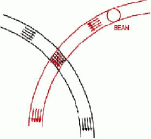
Averaging over the 60 scans of the same circle suppresses most noise with frequencies smaller than the spinning frequency. The remaining noise can be described by 1 offset per ring for each of the 3 Stokes parameters, irrespective of the number of polarized detectors. The circles have many intersections with each other in the sky. At these circle crossings (see figure 1), one can use the redundancy by asking that the sky Stokes parameters be the same along both circles. This results in solving a linear system with the Stokes parameter offsets as variable.
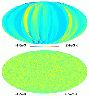
The coefficients of the residual maps before and after destriping (right panel)
The quality of the ”destriping” can be seen on figure 2. For further details, see [Revenu et al.(2000)].
3 Some useful definitions
Let us consider a “Polarization Sensitive Bolometer (PSB)”. The path followed by the incoming radiation is illustrated in figure 3.
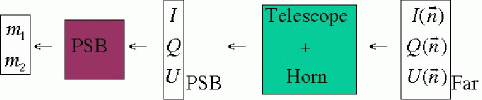
The far field Stokes parameters are integrated by going through the telescope and the horn to give the Stokes parameters on the PSB, :
| (1) |
In principle the 9 real functions are needed to characterize the beam completely. For a PSB at the center of a perfect instrument, only , and are present. The signals measured by the two detectors of the PSB are given by:
| (2) |
where is the rate of cross polarization leakage: if the
incoming radiation is not polarized, is the ratio of the
transmitted intensity polarized in the wrong direction to that
polarized in the right direction. The angles
() are the angle between the polarised sensitive
direction 1 (2) and the () axis of the local reference
system. Ideally these two directions are exactly orthogonal and one
can choose the local reference frame so that
to remove the contribution of
, and make the three coefficients and
irrelevant.
The gain factors and are in general different.
4 Uncertainties on polarization leakage and polarizers orientations
Uncertainties on the characteristics of the polarimeters will generate systematic errors. We focus here on two specific examples:
-
1.
The cross-polarization leakage in equation (2) is only known up to some uncertainty.
-
2.
The polarimeter orientation in the sky The angles and in equation (2) as well as the relative orientation of the two PSB’s necessary to measure the 3 Stokes parameters are not exactly known either.
We have evaluated these effects as follows
i)
Assume a “theoretical setup” of polarimeters with given rates
of cross-polarization leakage and given orientations in the sky.
ii) Assume that, due to imperfections in building the instrument, the
actual set up is different. An “actual setup” is built by adding random
errors to the cross-polarization leakage and to the polarimeter
orientations.
iii) Observe a set of Stokes parameters with the
“actual setup”
iv) Reconstruct the Stokes parameters using the “theoretical
setup”
v) Compare the original and reconstructed Stokes parameters for a
random sequence of “actual setups”.
The results are displayed in tables 1 and 2 ,
obtained with 4 polarimeters, K, K. Note that a known rate of cross-polarization
does not contribute to the systematic error but increases the statistical
uncertainty by a factor
| RMS error on | Relative | average error |
|---|---|---|
| leakage rates | RMS error on | on reconstructed |
| reconstructed polarization | polarization direction | |
| 0.01 | 1.4% | 0.2∘ |
| 0.05 | 7% | 2∘ |
| 0.1 | 15% | 4.5∘ |
| 0.2 | 35% | 8∘ |
| RMS error on | Relative | average error |
| polarimeters orientations | RMS error on | on reconstructed |
| reconstructed polarization | polarization direction | |
| 0.1∘ | 0.2% | 0.1∘ |
| 0.5∘ | 1% | 0.5∘ |
| 1∘ | 2% | 0.9∘ |
| 2∘ | 5% | 2∘ |
| 5∘ | 12% | 5∘ |
| 10∘ | 24% | 10∘ |
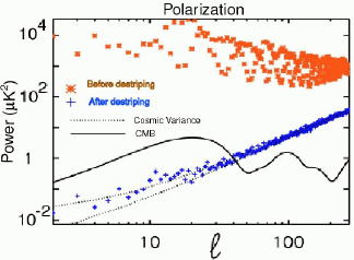
In order to check that the above uncertainties do not impact on our ability to measure polarized power spectra, we can test the effect of an imperfect knowledge of polarimetric calibration parameters in yet another way: a sky map simulated from a set of and spectra is observed with the “actual setup”. The map is then destriped as described above and reconstructed using the “theoretical setup”.
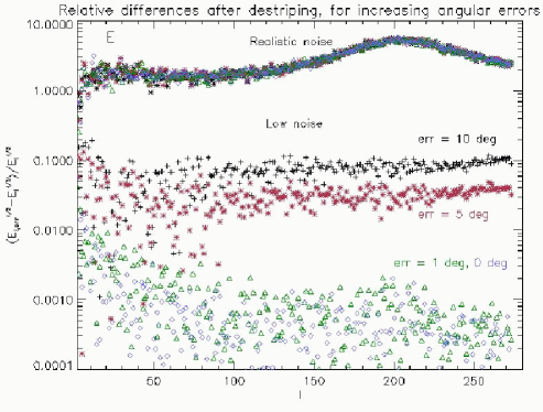
Finally the and spectra of the reconstructed maps are computed and compared with the inputs. Figure 4 shows the result of this comparison on the spectrum for random orientation errors of order 0 to 10 degrees. With a realistic noise the effects cannot be seen, therefore, the points labelled “low noise” have been evaluated with a noise divided by . With a error, the relative systematic errors on the spectrum remains below 1% (actually closer to 0.1%). The same results apply to the spectrum.
5 The crucial problem: Signal differences
As the and parameters are computed by differences between detector outputs, any mismatch between the characteristics of the detectors (gain, beam, pointing …) induces a fake polarization signal.
5.1 Relative photometric calibration between polarimeters (cross-calibration)
The gains and in equation (2) are in general different. This mismatch should be evaluated and corrected for by cross-calibration. A residual cross-calibration error will result in a spurious polarization signal . The and fluctuations induced in this way are strongly correlated to the temperature fluctuations. For the CMB, a 1% calibration error typically induces a 10%-30% systematic error on the polarization fluctuation. A constant calibration mismatch is easily detected and corrected for. The trouble comes from gain variations with time. The time scale for cross calibration have to be very carefully chosen. This question is currently under investigation on the polarized data from the Archeops flight in January 2000. Archeops is a balloon experiment to observe CMB fluctuations with an angular resolution around 10’. It involves 21 bolometers at 143, 217, 353, and 545 GHz. The 6 bolometers at 353 GHz are polarized and arranged in 3 Ortho Mode Transducers. After a technical flight in 1999, the first scientific flight occurred in January 2000 from the ESRANGE base at Kiruna in Sweden, and the data are currently being analyzed. Two more flights are planed in December 2001 and January 2002. (see Ref. [Benoît et al.(2001)] for more details).
5.2 Pointing and/or beam shape mismatch
The two orthogonal detectors necessary to obtain the (or ) parameter from the difference of their outputs should look at the same area of the sky. However, this will in general not be true. Ortho Mode Transducers (OMT) or Polarized Sensitive Bolometers (PSB) (see the contributions of the SPORT and BOOMERANG teams to this workshop) are a nearly perfect answer to this problem as the polarization signal is the difference between the outputs of two detectors sitting behind the same feed. However, even in this case a pointing mismatch can occur if the time constants of the 2 detectors are not the same.
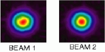
This is illustrated in figure 5: in the Planck mission, a 1 ms difference in the time constants of the two orthogonal detectors induces a 0.5’ pointing mismatch in the scanning direction. A beam shape mismatch can arise for the same reason and also because the two polarimeters are not oriented in the same way with respect to the horn and the telescope.
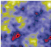
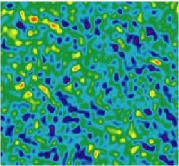
In figure 5, a temperature map with a dispersion
and zero
polarization (left panel), is observed with two orthogonal polarized
detectors. The center panel shows the map induced by a pointing
mismatch of 0.5’ between the two beams, otherwise identical (Gaussian and 7.5’ wide). The output
map develops fluctuations with , correlated
to the temperature signal. This level is large and only slightly
smaller than the expected polarization level of CMB fluctuations.
Note that for beams and beam mismatches small compared to the typical CMB
structures, the effect grows linearly with the distance between the
two beams.
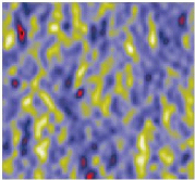
The right panel shows
the map generated by observing the same input temperature map with
the two mismatched beams shown in figure 6. The two beams
differ by 2.5% on 1/3 beam size scales. In this case the Q
fluctuation has .
6 Optimized polarimeter configurations
Because of the low signal to noise ratio, an elliptic error box in the plane can induce a bias on the polarimeter direction. An elliptic error box means unequal and/or correlated errors on and .
It can be shown [Couchot et al.(1999)] that a circular error box is obtained if
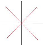
i) the polarizer orientations are evenly distributed over
180∘, as in figure 7 for 4 polarimeters
ii) the noise level should be as homogeneous as possible and
uncorrelated among the polarized detectors.
If these conditions are realized, one get as a bonus that the volume of the error box in the Stokes parameter is minimal. Of course, this second condition will be the most difficult to realize in practice.
7 Conclusions
In an experiment such as Planck HFI, where polarization measurements are made with detectors sensitive to the total polarized intensity in one direction, the main source of systematic error in polarization measurements is the fact that and Stokes parameters are obtained from signal differences. This can be overcome and even turned into an advantage if the systematics are common to both detectors with the same size and therefore disappear in the difference.
OMT’s and PSB’s are a partial answer to this requirement as the two detectors have nearly the same lobes and pointings. However the electronic chains (and part of the optics for OMT’s) are different. Moreover one still has to combine the signals of two different feeds to get the full polarized information. This latter combination is less dangerous however, as it does not involve intensity differences, and therefore will not generate polarisation where there is none.
A rotating polarizing device in front of one bolometer in one feed and read by one electronic chain may provide a solution to these difficulties, but one has to check that it does not bring new systematics and it may be difficult to implement on satellite or balloon borne experiments.
References
- [Revenu et al.(2000)] Revenu, B., Kim, A., Ansari, R., Couchot, F., Delabrouille, J., and J., K., A&ASS, 142 (2000), astro-ph/9905163.
- [Benoît et al.(2001)] Benoît, A., et al., To appear in Astroparticle Physics (2001).
- [Couchot et al.(1999)] Couchot, F., Delabrouille, J., Kaplan, J., and Revenu, B., A&ASS, 135, 579 (1999), astro-ph/9807080.