Looptop Hard X-ray Emission in Solar Flares: Images and Statistics

Abstract

The discovery of hard X-ray sources near the top of a flaring loop by the HXT instrument on board the YOHKOH satellite represents a significant progress towards the understanding of the basic processes driving solar flares. In this paper we extend the previous study of limb flares by Masuda (1994) by including all YOHKOH observations up through August 1998. We report that from October 1991 to August 1998, YOHKOH observed 20 X-ray bright limb flares (where we use the same selection criteria as Masuda), of which we have sufficient data to analyze 18 events, including 8 previously unanalyzed flares. Of these 18 events, 15 show detectable impulsive looptop emission. Considering that the finite dynamic range (about a decade) of the detection introduces a strong bias against observing comparatively weak looptop sources, we conclude that looptop emission is a common feature of all flares. We summarize the observations of the footpoint to looptop flux ratio and the spectral indices. We present light curves and images of all the important newly analyzed limb flares. Whenever possible we present results for individual pulses in multipeak flares and for different loops for multiloop flares. We then discuss the statistics of the fluxes and spectral indices of the looptop and footpoint sources taking into account observational selection biases. The importance of these observations (and those expected from the scheduled HESSI satellite with its superior angular spectral and temporal resolution) in constraining acceleration models and parameters is discussed briefly.

Subject Headings: Sun:flares–Sun:X-rays–acceleration of particles

1 INTRODUCTION

The discovery of hard X-ray sources located at or above the top of solar flare loops by the HXT instrument on board the YOHKOH satellite has provided great insight into the processes that drive solar flares. The canonical event for this phenomenon is the flare of January 13, 1992, first described by Masuda et al. (1994), and later analyzed by Alexander & Metcalf (1997), and is commonly referred to as the “Masuda” flare. This flare, which is clearly delineated by a soft X-ray (thermal) loop, shows three compact hard X-ray sources, two located at the footpoints (FPs for short) and a third above the top of the soft X-ray loop. The first systematic study of such sources was undertaken by Masuda (1994). During the period of time between the satellite’s first scientific observations (October 1991) up to September 1993, Masuda selected 11 X-ray bright limb flares observed by YOHKOH that met his selection criteria (see below), one of these 11 events was interrupted event and was not analyzed further. Of the remaining 10 flares, 6 demonstrated a nonthermal looptop (LT for short) source while another demonstrated what Masuda termed a “super hot” thermal LT source. This indicates that LT hard X-ray emission is fairly common. This view is strengthened further considering the limited dynamic range of the HXT instrument and the result we describe in this paper. Thus, it is reasonable to conclude that LT sources are present in all flares.

It is generally agreed that the primary energy of solar flares must come from reconnection of stressed magnetic fields, and as pointed out by Masuda et al. (1994), the YOHKOH LT observations lend support to theories that place the location of energy release high up in the corona. The energy released by reconnection can be used to heat the ambient plasma and/or to accelerate electrons and protons to relativistic energies. The power law hard X-ray spectra seen in many of the LT sources indicate that nonthermal processes, such as particle acceleration, are indeed occurring at or near these locations. The exact mechanism of the acceleration is a matter of considerable debate. In previous works (see Petrosian 1994 and 1996) we have argued that among the three proposed particle acceleration mechanisms (electric fields, shocks, and plasma turbulence or waves) the stochastic acceleration of ambient plasma particles by plasma waves provides the most natural means of explaining the observed spectral and spatial features of solar flares.

In two recent works (Petrosian & Donaghy, 1999 and 2000, hereafter PD) we demonstrated how the power-law spectral indices and emission ratios (obtained by Masuda 1994) can be used to constrain the model parameters. In this paper, we expand and extend Masuda’s analysis for further investigation of the ubiquity and nature of the LT source, and to gain a clearer picture of the range of values of the fluxes and spectral indices of the FP and LT sources. Furthermore, we investigate the temporal evolutions of the images of several new flares observed by HXT to determine the relationship between the many spatially and temporally distinct sources that occur in complex flaring events. In the next section we describe our procedure, and in §3 we present the light curves and images of most of the new events, including three events which appear to be examples of multiple loop flares. In §3 present the statistics of the relative fluxes and spectral indices of the LT and FP sources. In §5 we present a summary and our conclusions.

2 PROCEDURE

In seeking to expand the sample of flares with looptop emission, we have searched through “The YOHKOH HXT Image Catalog” (Sato et al., 1998) for appropriate limb flares using Masuda’s two criteria:

1) Heliocentric longitude $>80\arcdeg$; this ensures maximum angular separation between LT and FP sources.

2) Peak count rate in the M2 band $>10$ counts per sec per subcollimator (cts s^-1 SC^-1, for short); this ensures that at least one image can be formed at high energies ($\sim 33-53$ keV) where thermal contribution is expected to be lower.

In total, we found 20 events from October 1991 through August 1998 that satisfy these conditions. Of the events before September 1993 (when Masuda stopped his search), we found 12 such flares, including 11 events noted by Masuda and one event (that of December 18, 1991) which satisfies the search criteria but was apparently overlooked by Masuda. From the period after September 1993 up to August 1998 (when the image catalog was finished) we have an additional 8 events. In the interest of completeness we include all twenty events in this survey (see Table 1). However, two events (November 2, 1992 noted but not analyzed by Masuda, and May 10, 1998) have their observations interrupted by spacecraft night, and we are unable to obtain any useful information from them. An interesting aside (which we shall return to in §4), is that of the 9 new events, 3 appear to be examples of interacting loop structures with multiple LT and FP sources, of the type analyzed by Aschwanden et al. (1999). It is surprising that none of the 11 Masuda events are in this category. It should also be noted that three of the flares observed before September 1993 show no detectable LT emission, while all of the flares since that date (with the exception of one ambiguous source) show LT emission.

For the ten early events, Masuda quotes LT and FP spectral indices for the events when those sources are detected, although he does not supply the time intervals or spatial regions over which the indices are taken. Masuda obtains two spectral indices by fitting a power law to the L ($\sim 13-23$ keV) and M1 ($\sim 23-33$ keV) band fluxes, and the M1 and M2 band fluxes. We carry out spectral fitting both to a simple power law as well as a broken power law using all four channel fluxes (including the H band with energy range $\sim 53-93$ keV), whenever significant fluxes in all four bands are detected. These results are summarized in Tables 2 and 3.

For two events (January 13, 1992 and October 4, 1992), Masuda performs a temporal and spatial analysis, providing light curves for emission from the LT and FP regions. He defines a box around each source, with size and center position determined from the best available image, and then obtains light curves by measuring the total flux of photons coming from within the box as a function of time. We undertake this temporal analysis for all the events in our list for which the necessary data are available. The data reduction is done with the standard YOHKOH HXT software package, which uses the maximum entropy method (MEM for short); in particular we use hxt_multimg, lcur_image, and hxt_boxfsp routines.

Event #	Date	Peak Time	Disk	GOES	L band	Loop Top
		hhmmss	Position	Class	Peak Count	Location
1	91/12/02	045527	N18E84	M3.6	61	inside*
2	91/12/15	024411	——	M1.2	30	NO SXT
3	91/12/18	102740	S14E84	M3.5	379	inside(New)
4	92/01/13	172937	S16W84	M2.0	51	above*
5	92/02/06	032511	N06W84	M7.6	807	inside(s-hot)
6	92/02/17	154209	N16W80	M1.9	33	inside
7	92/04/01	101407	——	M2.3	50	no LT source*
8	92/10/04	222107	S05W90	M2.4	35	above
9	92/11/02	030002	S24W84	X9.0	11608	Int.
10	92/11/05	061959	S18W84	M2.0	68	none
11	92/11/23	202602	S08W84	M4.4	94	NO SXT
12	93/02/17	103630	S07W87	M5.8	229	above
13	93/09/27	120839	N08E84	M1.8	70	above
14	93/11/30	060337	S20E84	C9.2	57	C
15	98/04/23	054454	S20E84	X1.2	1496	single*
16	98/05/08	015847	S16W84	M3.1	116	C
17	98/05/09	032641	S16W84	M7.7	860	NO SXT
18	98/05/10	131849	S28E84	M3.9	138	Int.
19	98/08/18	082141	N34E84	X2.8	3499	inside?
20	98/08/18	221534	N30E84	—-	12397	C

Table 1: List of events from October 1991 to August 1998 that satisfy Masuda’s two criteria. Dates, UT times, position on the solar disk, flare classifications and the Peak Counts in the L band (columns 2 to 6) are taken from Sato et al. (1998). Column 7 describes the location of the LT HXT source relative to the SXT loop and some other characteristics of the images. The horizontal line divides the Masuda (pre September 1993) flares and our post September 1993 flares. Flares identified by a * may be partially occulted by the solar limb. NO SXT implies absence of SXT image of the loop. Flare # 3 labeled (New) was missed by Masuda. Flare # 4 was classified by Masuda as a super-hot thermal source. Flare # 15 (identified as single*) shows presence of only one resolved source which may be the LT source of an occulted loop. C=complex multiple loop event. Int.= Interrupted observation, not analyzed.

For several events, we have performed image reconstruction using both the standard MEM routine as well as the “pixon” technique used by Alexander & Metcalf (1997). As described in that paper, the “pixon” routine achieves significantly better photometry of faint sources and better rejection of spurious sources than the standard MEM routine, albeit with a significantly longer computational time. These features are useful to our analysis since we are often attempting to resolve a faint LT source in the presence of much stronger FP sources. In general, the “pixon” and MEM analyses yielded similar light curves.

Major sources of systematic uncertainty in our analysis arise from the difficulty in defining exactly what constitutes a LT or a FP source. In many cases, one or more of these sources will be quite strong and well localized at one epoch during a flare but they may disappear, change position or combine with another source as the flare evolves. Therefore, the procedure of integrating the fluxes using a static box to obtain a light curve for the duration of the flare can lead to erroneous conclusions because of the possibility of contamination of one source by neighboring sources. Further errors arise from the fact that in many flares nonthermal emission, which tends to be more impulsive and and peak earlier is superimposed upon the more gradual thermal emission which peaks later. Therefore for the study of the impulsive component (as a means of studying the acceleration mechanism) we limit our analysis of the flux ratios or spectral indices to the early stages of the flares to minimize the influence of the thermal component. We also use the M1 channel (rather than the L channel) where the thermal effects are expected to be smaller. Clearly it would be safer to use channels M2 and H, but these channels have weaker emissions.

3 CASE STUDIES OF IMAGES AND LIGHT CURVES

In this section we present light curves and a brief analysis for all of the newly analyzed events. Unless otherwise noted, the image and light curves were taken in the M1-band and using the standard MEM procedure.

3.1 Single Loop Flares

Of the 18 total events, 11 appear to by morphologically similar to the canonical “Masuda event”, that is, a single flaring loop anchored by twin FPs and exhibiting a distinct LT source. Of course, within this type we observe a good deal of variation. We present a few case studies.

December 18, 1991 – This event occurred during the early phases of the YOHKOH mission, but for reasons unknown to us it was not selected or analyzed by Masuda. The hard X-ray images initially show one bright source (at around 10:25:00), which could be either a LT or a FP source, coaligned with the bright region of the soft X-ray flaring loop. Shortly after the start of the flare, the single source splits into two, and sometimes three, unresolved sources coaligned with the flaring loop. The loop joining sources A, B and C, in the right panel of Figure 1, is most likely an asymmetric loop. This can give rise to the observed differences between the intensities and heights above the solar limb of the two FP sources B and C. The left panel of Figure 1 shows the light curves for each of these three regions. The dominance of the source A during the initial peak of the flare could be due to efficient trapping of the accelerated electrons at the acceleration site (assumed to be at the top of the loop) by a high density of plasma turbulence. Therefore, we assume it to be a LT source for this analysis. Note that for this flare the ratio of the sum of the counts of the two FPs to that of the LT source, ${\cal R}=FPs/LT$, is about one, changing from 0.6 at the beginning to $\sim 1.2$ during the main pulse. In our statistical analyses described in the next section we will often use the counts $FPs$ and $LT$ of the main pulse, and in few cases we use the counts of well defined pulses separately. We will rarely use the counts or the ratios obtained during the decaying phase where thermal contamination may become large. The “pixon” reconstruction of the same event shows cleaner images, but the same light curves.

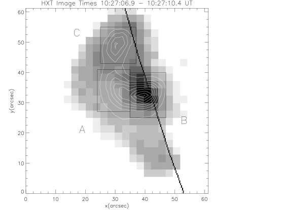
Figure 1: Images (right panel) and light curves (left panel) for the December 18, 1991 flare. The contours and the gray scale show the HXT (channel M2; 33-53 keV) and SXT images of the loop, respectively, for the specified time. The diagonal line shows the location of the solar limb. The brightest contour in the HXT image is at $B_{max}=8.1$ counts/pixel with 2.5 sq arc second size pixels, and the contour separations are $\Delta B=0.73$ counts/pixel. The light curves of the the LT and FP sources refer to the counts integrated over regions shown on right panel. The dashed histogram shows the average of the ratio of counts of two FPs to the LT sources, ${\cal R}=FPs/LT$ (multiplied by 10) for three time intervals.

September, 27, 1993 – The SXT images for this event show a compact flaring loop on the limb and the HXT images primarily show two bright FPs associated with this loop. The LT source is weaker (the count ratio ${\cal R}\sim 8$) and appears only intermittently high above the flaring loop in the corona. However, as shown in Figure 2 the LT and FP sources have similar pulse structures.

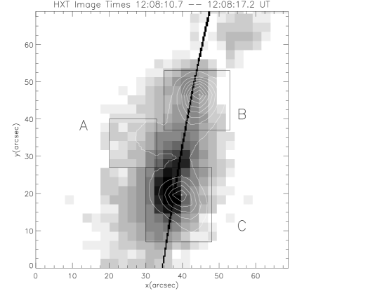
Figure 2: Same as Figure 1 for the September 27, 1993 flare, with $B_{max}=4.1$ and $\Delta B=0.41$ counts/pixel.

August 18, 1998, 08:21UT – This very bright X-class flare is the first of two bright flares from this active region on this day. The SXT images show a bright loop structure that is coaligned with two FP HXT sources and one bright LT HXT source, Figure 3. These three sources persist throughout the impulsive phase of the flare and share common impulsive peaks. In the late phase (after 08:20:15), the LT comes to dominate and the HXT emission becomes more localized. In contrast to the preceding flare, the LT source here is extremely bright and long lived.

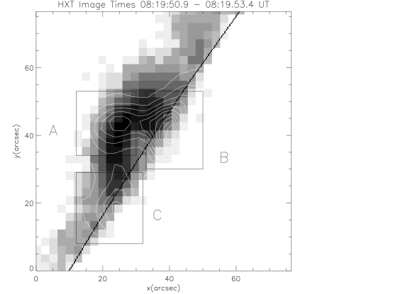
Figure 3: Same as Figure 1 for the first August 18, 1998 flare, with $B_{max}=1.9$ and $\Delta B=0.15$ counts/pixel.

Taken together with the “Masuda flare” of January 13, 1992 and the other single loop flares analyzed by Masuda, we note that the LT can manifest itself in many different forms. Some flares only show LT emission very briefly or very faintly. In larger flares, we observe LT sources that are clearly spatially separated from the FP sources, yet have similar impulsive time structure.

3.2 Multiple Loop Flares

Three of the post 1993 flares we have analyzed show HXT (and SXT) images with complex morphologies that have strong fluxes coming from several distinct regions which brighten and dim at different times. These flares cannot be modeled by a single loop and provide evidence for existence of multiple loop structures. It should be noted that none of the pre 1993 flares showed such complex structures.

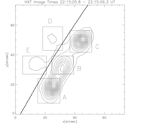
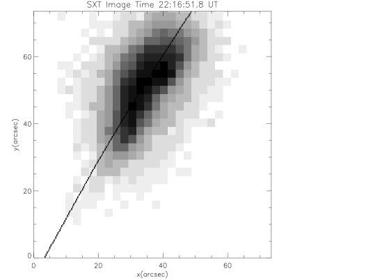
Figure 4: Same as Figure 1 for the second August 18, 1998 flare. The upper left and right panel light curves represent the southern (AEB) and the northern (BDE) loops, respectively. Note that for the LT source D we plot counts divided by 3. In the HXT image (lower left panel) $B_{max}=14.8$ and $\Delta B=0.82$ counts/pixel. The SXT image is shown separately on the lower right panel to avoid confusion. (Note that the SXT image is taken nearly two minutes after than the HXT image. This can explain the misalignments between the two images.) The digonal lines in the images show the location of the limb.

August 18, 1998, 22:15 UT - This event (see Figure 4) is the second flare occurring on this day in this active region, and it is one of the most energetic flaring events observed since YOHKOH’s launch. This X-class flare appears in the hard X-rays as two flaring loops sharing a common central FP, but is too bright for most of the flare duration to yield useful images in soft X-rays. The early SXT images have many overexposed pixels and the later images show only one flaring loop associated with the upper two FPs. The upper loop is associated with two bright FPs (B and C), and a loop top source (D), which shows impulsive behavior superimposed upon an extremely hot thermal component (seen even in the M2 band). A third FP source (A) lies further south from the soft X-ray flaring loop and is associated with a comparatively fainter LT source (E) situated between it and the middle FP. The light curves give evidence for multiple acceleration sites. For example, while all three FPs participate in the first large peak (just after 22:15:05), only the upper sources show strong emission at the later peaks (22:15:30 and 22:15:50), while the lower sources fade away.

May 8, 1998 - Figure 5 shows hard X-ray image (at 01:57:40) and the corresponding light curves for this flare. The light curves and images presented here are from the “pixon” reconstruction method, which can identify faint sources better than the MEM method. Evidence from the soft X-ray images points to the existence of two flaring loops which share the lower FP (denoted B in the figure) and whose LT sources (E and C) overlap. The smaller loop is brighter and is associated with the FPs B and D and the LT source, E. The fainter, outer loop is associated with B and the considerably fainter FP source, A, as well as the LT source C. While two upper FP sources (D and A) are indeed fainter, they do demonstrate the same impulsive variation as their brighter LT and FP relatives. Looking at the light curves, we can see that the inner loop is strongly associated with the first impulsive peak at 01:57:30. The outer loop peaks later (at 01:58:30), at a time which coincides with a low point in the light curves of the inner loop sources. It is difficult to demonstrate the presence of a causal connection, if any, between these loops. The time profile of source B is approximately a superposition of the time profile of the two FPs A and C that are separated spatially and temporally.

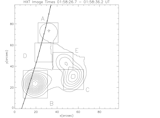
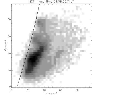
Figure 5: Same as Figure 4 for the May 8, 1998 flare. The upper left and right panel light curves represent the inner (DEB) and the outer (ACB) loops, respectively. In the HXT image $B_{max}=3.0$ and $\Delta B=0.23$ counts/pixel. These images were reconstructed using the “pixon” method.

November 30, 1993 - This event appears as a double loop structure in soft X-rays with apparent multiple LT and FP sources appearing in the hard X-ray images.

This flare was analyzed by Aschwanden et al. (1999) in their study of quadrupolar magnetic reconnection events. Aschwanden et al. analysis shows presence of only a double loop with the lower FP common to both the larger outer loop and the smaller inner loop. Our analysis of this flare using the “pixon” method resulted in images that were considerably cleaner than those from the MEM technique. In Figure 6 we present a map of the X-rays images as well as light curves for the selected sources obtained from the “pixon” method. Based on these one may deduce that there are three separate loops BGC, AFE and ADC with common FPs A and C having composite time profiles.

However, the basic structure of the flare remains complicated. In the early stages of the flare there are actually four FP HXT sources that correspond to four bright spots in the SXT images (sources A, B, C & E in the figure). More confusing is the behavior of what appear to be three separate sources appearing high in the corona (sources D, F & G). The fainter source (D) appears early in the flare at the very top of the loop, while the two stronger sources (F & G) appear later and at lower altitudes. As the flare evolves, all of these FP and LT sources shift their position with respect to each other, making it very difficult to perform the usual analysis. A comparison of the light curves for sources A, C & D (the outer loop), shows that they peak at similar times early in the impulsive phase. However, the peaks of the light curves for other sources are not correlated as clearly, and have extremely complicated structures. For example, a late peak of source B does not appear in any other source. Note also that the LT sources in this flare are much weaker than the FP sources.

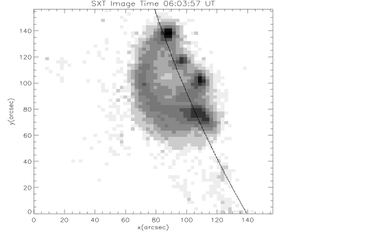
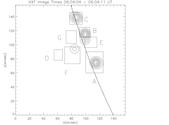
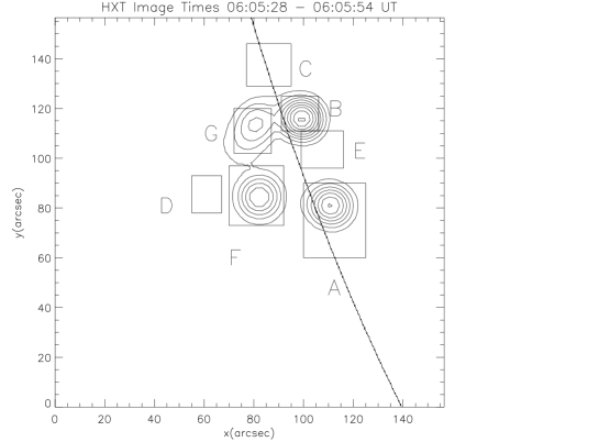
Figure 6: Same as Figure 4 for the November 30, 1993 flare. The light curves in the middle left panel represents what may be the outer flaring loop (ADC), while those in the upper two panels represent other sources seen in the flare, which may form two inner loops (CGB and EFA). The SXT image is shown in middle right separately and two HXT images at two different times are shown at the lower panels, with $B_{max}=2.5$ and $\Delta B=0.23$ counts/pixel for the left panel, and $B_{max}=1.7$ and $\Delta B=0.16$ counts/pixel for the right panel. These images were reconstructed using the “pixon” method.

3.3 Miscellany

April 23, 1998 – This flare appears in the soft X-ray images as bright diffuse emission above the solar limb, accompanied by thin, quickly evolving loop structures that are probably not the main flaring loop. The HXT emission initially appears in two sources, but quickly become one undifferentiated source associated with the bright diffuse soft X-ray emission. The lack of an observable flaring loop indicates the possibility that this flare occurred behind the limb and the emission we are seeing is very high up in the corona, rather than a single FP source (see Figure 8).

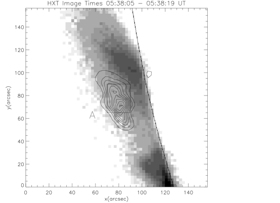
Figure 7: Same as Figure 1 for the April 23, 1998 flare, with $B_{max}=4.4$ and $\Delta B=0.40$ counts/pixel. The FP sources of this flare are most likely occulted and source A represents the LT source.

Figure 8: Same as Figure 1 for the May 9, 1998 flare, with $B_{max}=4.1$ and $\Delta B=0.31$ counts/pixel.

May 9, 1998 – This flare appears as a single FP and a LT hard X-ray source only during the initial two minutes of the flare (see Figure 8), when we see one strong FP accompanied by much fainter emission above it that may be a LT source. As the flare progresses, the FP source grows in intensity so much that the limited dynamic range of the HXT makes the detection of the much fainter LT signal impossible. The discrepancy between the positions of the SXT and HXT images is large, so that it is difficult to determine whether the observed HXT sources are associated with any SXT features.

4 STATISTICAL RESULTS

In this section we consider the statistical properties of the flares listed in Table 1 and summarize the differences between the original Masuda flares and the new events classified by us. In total there are 18 events for which we have sufficient data. Of these 15 show at least one impulsive source which can be classified as a LT source. Most of these can be classified as nonthermal, and one (the 920206 flare) is classified by Masuda as a “super hot” thermal LT source. The remaining three show no detectable LT emission. As we shall see below these non-detections are due to the shortcomings of the instrument indicating that LT emission is a general feature of solar flares. We discuss the statistics of two physical characteristics, namely the relative fluxes and spectral indices of the LT and FP sources.

4.1 Relative Fluxes

The most directly available data are the statistics of the relative values and distributions of the fluxes from the LT and FP sources. Theoretically, the relative values of these emissions are important for determination of the characteristics of the models. As shown in PD, the ratio of LT to FP emission can be related to the ratio of acceleration and diffusion rates of the electrons as well as the plasma density and magnetic field strength. Here, we examine the relative values of the LT and FP emissions for the entire sample.

In Figure 9, we plot the sum of the count rates (in units of cts s^-1 SC^-1) of the two footpoint sources ($FPs$) vs. the count rates of the corresponding looptop source ($LT$). The values shown in this figure refer to count rates (or fluxes) spatially integrated over each source, and integrated over the entire impulsive duration of each flare, or over individual pulses in flares where distinct pulses and loops are discernible. For three events, where multiple loop structures with corresponding LT and FP sources are observed (see §3), we plot LT and FPs fluxes for each loop as separate points but connect them with lines.

Figure 9: Counts from two FPs vs. LT counts, in the M1 band for all 18 flares in our sample. The diagonals represent lines of constant ratio (${\cal R}=FPs/LT$) and represent detection thresholds arising from the finite dynamic range of the instrument: Solid lines at 20 and 0.2 for two equal FPs; dotted diagonals for one dominant FP source. Flares with undetected LT source are denoted by an arrow placed on the upper bound of detection of ${\cal R}=10$. The dashed line shows the event selection threshold of 10 cts s^-1 SC^-1 at M2 band which on the average (see Fig. [10]) means $FPs+LT\simeq 5$ cts s^-1 SC^-1 for the M1 band. For uniformity, all the data points on this plot were obtained using the standard MEM reconstruction procedure.

The primary trend seen in this figure is an obvious correlation between FPs and LT fluxes over more than two decades of flux. The second striking feature is that for most flares (or pulses in flares) the ratio of these two fluxes is confined to $1<{\cal R}=FPs/LT<10$. Only three events lie beneath the line of equality (the thick solid line). The presence of an upper envelope is most likely an artifact of the limited dynamic range of the instrument and the image reconstruction process (estimated to be about one decade), and is not an intrinsic feature of the flare emission. This limitation means that for two FPs with equal fluxes the plotted ratios will lie in the range $20<{\cal R}<1/5$ shown by the two thin solid diagonal lines. But if one FP is much stronger than the other, then the above ratio should lie in the range $10<{\cal R}<1/10$, shown by the dotted lines. (Because of the limited dynamic range, the weaker FP source cannot be more than ten times weaker than the stronger one. Hence, strictly speaking the latter limits should be 11 and 0.11.) Since the LT source that is 10 or 20 times weaker than the accompanying FPs would not be detected by the HXT instrument, or revealed by the image reconstruction process, we show the three events with no detectable LT emission with horizontal arrows starting at the ${\cal R}=10$ line, which assumes equal counts for the two FPs. Similarly, events falling beneath the ${\cal R}=0.1$ (or 0.2) line will not have a detectable FP emission. There is only one flare with the ratio approaching this value. This is the April, 24 1998 flare, shown by a vertical arrow in Figure 9. This and one of the other two events below ${\cal R}=1$ line, the December 2, 1991 flare, are believed to have occurred behind the limb, so that the FP sources are fully or partially occulted, giving it an abnormally low flux ratio. (Masuda mentions that two other events, January 13, 1992 and April 1, 1992, may also have occurred behind the limb.) The other flare below the ${\cal R}=1$ is the February 6, 1992 event, which according to Masuda shows a (super-hot) thermal spectrum for the LT and FP sources. Our spectral analysis shows a very steep spectrum for these sources (see Table 3 below) supporting this assertion. The Dec. 18 1991 event, missed by Masuda, also shows a very steep spectrum for both LT and FP sources (see Table 3 below) and lies near the equality line ${\cal R}=1$.

We therefore conclude that the absence of events below the line of equality (${\cal R}=1$) is not an instrumental effect and must be intrinsic to the flare process. It should be reemphasized that the limitations introduced by the dynamic range will also bias the data in favor of events with FP flux ratios of less than 10. Those with greater ratio will appear as a double (FP and LT) or just a single (FP) source depending on the strength of the LT source. We also note that for some, but not all, events with multiple pulses and or multiple loops, the data points from different loops or pulses lie near each other (e.g. October 4, 1992 and May 8, 1998). Interesting exceptions are the flare on November 23, 1992, which exhibits one pulse with a significantly lower value of ${\cal R}$ than the other two pulses, and the flare on May 9, 1998, where a LT source is detected during the first pulse, but not during the later, much stronger pulse (which we show in Fig. 9 with an upper bound for the LT source).

We must also consider the truncation introduced by our selection criteria. Because of the threshold of 10 cts s^-1 SC^-1 imposed by us (and Masuda), only flares with the flux (in M2 band) of $(FPs+LT)>10$ cts s^-1 SC^-1 will be in the sample. We estimate below that this translates to a threshold of 5 cts s^-1 SC^-1 for the M1 band. This truncation boundary is shown by the dashed curve in Figure 9. As is evident, all flares except the 911215 flare fall above this boundary.

In addition to the bounds derived from our selection criterion and the finite dynamic range, there is also an absolute bound below which the instrument sensitivity drops rapidly. Since the HXT detection of flux is not based in a well defined trigger process, we attempt to determine this bound by studying the distribution of flare peak count rates using the entire HXT database of 1307 flares over the same time period. In Figure 10, we plot the differential distribution of flare peak count rates for each of the HXT four channels and for the summed over four channel peak count rate. From each count rate we subtract a representative background count rate for the channel. Sato et al. (1998) give approximate background count rates of $L\simeq 2$, $M1=M2\simeq 1$, $H\simeq 9$ cts s^-1 SC^-1. As is evident, the distributions roughly follow a power law, especially at high and midrange values, in agreement with many previous flare surveys (see Lee & Petrosian 1995 and reference cited there). We also plot the power law distributions from linear regression fits to the distributions from M1, M2 and total peak count rates and give the power-law indices (i.e. logarithmic slopes). The slope values of $\sim-0.6-0.8$ obtained here are consistent with previous results (Lee & Petrosian 1995) and shows that YOHKOH flares do not suffer from additional biases and that our results regarding the LT emission is applicable generally to all flares. The flattening away from the power law at low count rates is due to a decrease in the sensitivity of the detectors. This is especially prominent in the L channel, because of its higher background rates. For the M1 and M2 bands there seems to be very little flattening down to the quoted background value of 1 cts s^-1 SC^-1. Note that the M2 and M1 band distributions are shifted relative to each other horizontally (and vertically too) by an approximately constant value of about 2. This means that the average threshold value of the M1 cts s^-1 SC^-1 for our sample is about 5. This value was used in determining the truncation boundary in Figure 9 (the dashed line).

Figure 10: The differential distribution of peak counts of all the flares for the entire mission (October 1991-August 1998), for the sum and each of the four channels (bands L, M1, M2 and H, from top to bottom) of the HXT instrument. For clarity the histograms are shifted vertically by the indicated factors. The straight lines show the linear regression fit for each histogram. The values of the slopes $\gamma$ are -0.73, -0.63 ,-0.76, -0.80 and -0.73 from top to bottom, respectively.

In summary, from the above analysis of the relative strengths of the LT and FP fluxes we can conclude that the hypothesis that all flares have LT emission is consistent with the extant, though limited, data. Figure 11 shows the distribution of ${\cal R}=FPs/LT$ for the flares presented in Figure 9. This distribution if fairly flat between 0.5 to 8 and there are four flares with undetected LT emission (i.e. ${\cal R}>10$) as shown by the arrows. Obviously the statistical significance of these data point is marginal and a more quantitative account of the relative distributions of the fluxes of the LT and FP sources requires a larger sample and dynamic range. Nevertheless, this kind of data is very important and can constrain the model parameters. As described in PD this ratio can be related to the acceleration and the background plasma parameters. For example, it was shown that under certain conditions one has ${\cal R}=\tau_{\rm Coul}/T_{\rm esc}$, where $\tau_{\rm Coul}$ and $T_{\rm esc}$ are the Coulomb collision time scale in the loop and the escape time on the electrons from the acceleration site at the LT. However, for more general situation the relation of this ratio to the physical parameters si more complicated. As shown by numerical calculation in PD values of a few for this ratio indicate plasma densities of about few times $10^{10}$ cm^-3 and require a relatively short acceleration time compared to the escape time of the electrons from the LT source. Further constraints come from the consideration of the spectral shapes which we discuss next.

Figure 11: The differential distribution of the ratio ${\cal R}=FPs/LT$ of the footpoints to looptop peak counts of all the flares for the entire mission (October 1991-August 1998). The arrows indicate ratios greater than the dynamic range of about 10. Some of the flares in the shaded area may be occulted or be dominated by thermal emission from a superhot component.

4.2 Spectral Indices

Another characteristic of the LT and FP emissions which can shed light on the acceleration mechanism is the relative shape of their spectra. The HXT instrument observes only at four broad channels, so that an accurate, absolute spectral analysis of individual sources is difficult and results are uncertain. However, the relative spectral characteristics of FP and LT sources are more reliable. To this end we have carried out the following analysis. We use the YOHKOH routine hxtbox_fsp, which fits a specified model spectrum to the observed count rates and finds the best fit model parameters and calculates the chi-square’s. When possible, we attempted to measure the spectral shape early in the impulsive phase (before or right at the first impulsive peak) so as to minimize any thermal contributions to the spectrum.

For flare events with detectable images in the H band, we use the following four models:

1. A simple power law fitted to all four channels (Powerlaw1).

2. A simple power law fitted to the three highest channels (Powerlaw2) so that we avoid possible thermal contribution in the L band.

3. A broken power law with three parameters (low and high energy spectral indices, $\gamma_{1}$ and $\gamma_{2}$, and the break energy $E_{br}$) fitted to all four channels (Broken Powerlaw1).

4. Two simple power laws fitted separately to the L and M1 bands, and to the M1 and M2 bands (Broken Powerlaw2). In this case the break energy is fixed as the midpoint of the M1 band at $\sim 28$ keV.

Table 2 summarizes these results.

Event #	Date	Time	Source	Powerlaw1	Powerlaw2	Broken Powerlaw1	Broken Powerlaw2
				$\hskip 2.84526pt\gamma$     $\chi^{2}/\nu$	$\gamma$     $\chi^{2}/\nu$	$\gamma_{1}$     $\gamma_{2}$     $E_{br}$     $\chi^{2}$	$\gamma_{L,M1}$     $\gamma_{M1,M2}$
2	911215	02:44:09	A (FP)	6.1     21	4.5     5.8	–	6.8           3.8
			B (FP)	4.3     18	5.1     16	3.0     9.9     42     0.0	2.9           3.5
4	920113	17:28:04	A (FP)	3.5     2.2	3.8     0.32	–	3.1           3.9
			B (FP)	3.3     8.6	3.7     0.02	–	2.5           3.7
			C (LT)	5.3     12.8	6.6     0.45	–	4.2           6.8
7	920401	10:13:05	A (FP)	3.8     1.3	3.9     0.0	2.2     3.9     18     0.0	3.7           3.9
8	921004	22:19:31	A (FP)	4.7     21	5.9     0.01	–	3.2           5.9
			B (FP)	4.5     14	4.9     19	–	4.0           3.6
			C (LT)	5.8     0.61	5.6     0.85	5.8     7.6     56     1.1	6.0           5.3
10	921105	06:19:20	A (FP)	4.1     20	4.4     8.2	3.6     5.0     34     0.0	3.6           4.1
19	980818	08:19:13	A (LT)	7.4     32	7.4     64	–	7.4           7.7
			B (FP)	6.0     260	4.3     0.41	12     4.3     18     .45	6.6           4.2
			C (FP)	5.1     140	6.2     0.02	–	3.9           6.2
20	980818	22:14:36	A (FP)	3.1     590	3.5     200	2.3     3.9     32     0.0	2.2           3.1
			B (FP)	3.6     2.4	3.6     1.3	–	3.7           3.5
			C (FP)	3.5     17	3.4     1.9	5.6     3.4     18     1.9	3.7           3.4
			D (LT)	5.0     66	4.4     59	5.3     3.2     37     0.0	5.3           4.9
			E (LT)	3.8     32	4.0     43	3.2     3.8     9.7     63	3.4           4.4

Table 2: Spectral parameters from fits to four models of events with detectable H band images: Powerlaw1 uses all four channels (degrees of freedom $\nu=2$); Powerlaw2 uses the three highest channels ($\nu=1$); Broken Powerlaw1 uses all 4 channels ($E_{br}$ in units of keV); and Broken Powerlaw2 the three lowest bands with $E_{br}$ set to $\sim 28$ keV, the midpoint of the M1 channel ($\chi^{2}=0,\nu=0$). Missing spectral parameters for events in the Broken Powerlaw1 column indicate that the $\chi^{2}$ minimization for the spectra did not converge.

We first note that in 14 out of 18 cases the value of the reduced chi-square, $\chi^{2}/\nu$, is lowered when we remove the L band from the fit. The 4-channel fit chi-squares are lower, by statistically insignificant amounts, only for one FP and three LT sources. This combined with the results from the Broken Powerlaw2 fits indicates that deviations from a power law is produced by the L band and that these could be in form of a flattening or steepening of the spectrum with approximately equal probability. (The break energy $E_{br}$ distribution, however, does not seem too agree with this conclusion. Only 4 out of nine values fall in or near the L band. This could be due to statistics of small sample.) The observed spectral change, of course, is not a reflection of the true behavior of the spectra because flares with detectable H band flux must necessarily be biased toward those with flat and/or flattening spectra. Below we will compare the statistics of these flares with those without a detectable H band flux.

For flares with no useable images in the H band , we use two models; a simple power law fitted to the three channels (Powerlaw) and the model 4 above (Powerlaw2). Table 3 presents the results of this analysis.

Event #	Date	Time	Source	Powerlaw	Broken Powerlaw2
		hh:mm:ss		$\gamma$      $\chi^{2}/\nu$	$\gamma_{L,M1}$     $\gamma_{M1,M2}$
1	911202	04:53:45	A (LT)	6.2     0.6	6.3           5.9
			B (FP)	5.8     3.3	5.2           7.1
			C (FP)	5.4     0.01	5.4           5.3
3	911218	10:27:16	A (LT)	7.1     87	6.5           9.0
			B (FP)	6.2     46	5.8           7.1
			C (FP)	8.3     31	7.9           11
5	920206	03:22:16	A (LT)	8.1     320	6.8           12
			B (FP)	7.7     43	6.9           10
			C (FP)	8.3     56	7.6           11
6	920217	15:40:44	A (FP)	3.3     14	2.4           4.1
			B (LT)	6.2     31	6.9           3.1
			C (FP)	3.5     41	3.6           3.5
11	921123	20:24:39	A (FP)	3.7     1.7	3.5           3.9
			B (LT)	10       2.0	10           8.0
			C (FP)	6.4     3.2	6.7           5.5
12	930217	10:36:13	A (FP)	4.8     37	4.3           5.6
			B (FP)	6.5     42.	6.0           7.9
			C (LT)	6.2     12	5.8           7.0
13	930927	12:08:10	A (LT)	6.2     8.3	5.6           9.7
			B (FP)	4.9     20	4.1           7.2
			C (FP)	5.7     23	5.7           7.2
14	931130	06:03:33	A (FP)	2.7     37	1.6           3.5
			B (FP)	3.8     3.6	3.2           4.4
			C (FP)	3.5     74	1.3           5.7
			D (LT)	3.6     18	2.1           5.2
15	980423	05:38:46	A (LT)	7.5     5.2	7.4           7.8
16	980508	01:58:29	A (FP)	4.7     35	4.7           4.5
			C (LT)	5.8     22	5.0           7.5
		01:57:28	B (FP)	3.9     4.0	3.7           4.2
			D (FP)	4.2     19	3.3           5.5
			E (LT)	5.5     22	4.8           7.0
17	980509	03:19:36	A (LT)	6.6     5.2	6.1           7.9
			B (FP)	6.3     20	5.9           7.3

Table 3: Spectral indices of events wit undetected H band images from a simple powerlaw fit to three available bands ($\nu=1$) and from a broken power law fit, where we fix the break energy to correspond to the midpoint of M1 band at $\sim 28$ keV ($\chi^{2}=0$, $\nu=0$).

We first would like to note that the results from our analysis of the same events do not agree with Masuda’s numbers. This could be either because the HXT grid response functions have been improved since Masuda did his analysis (see Sato, Kosugi and Makishima 1999), or due to the differences in the spatial boxes or time intervals used to calculate the indices. Masuda does not specify these data. However, the general characteristics of the spectra (ranges, steepenings, etc.) of pre and post September 1993 bursts given in the above table agree with the the characteristics of ten pre September 1993 ten spectra cited by Masuda.

Second, we note that in contrast to the sample of Table 2, only two sources (LT sources in 920217 and 921123) in Table 3 show a significant flattening. The rest maintain the power law form, or in the majority of cases steepen by a significant amount (an spectral index change of greater than 1); the spectral index changing by more than 3 in some sources. This difference between the flares from Tabels 2 and 3 is due to the selection bias mentioned above and indicates that caution should be exercised in the interpretation of results from limited samples. The following figures describe the prominent features of the results from the whole sample.

Figure 12 shows the distribution of the spectral indices for FP (solid histograms) and LT (dashed histograms) sources from the simple power law fits, for events with no H band images (left panel) and events with H band images (right panel). Several features are readily apparent. First, the main difference between the two samples is absence of significant number of high spectral index ($\gamma\gtrsim 6$) events in the sample with H band images (6 vs 16 in the sample with no H band images) and a higher average spectral index, ${\bar{\gamma}}_{4ch}=4.65\pm 1.2$ vs ${\bar{\gamma}}_{3ch}=5.73\pm 1.5$. This is as expected. The HXT detects roughly equal counts in four channels from a flare with index $\gamma=4$. So that for $\gamma>6$ the counts in the H band will fall below that of the M2 band by a factor of 4. This combined with our chosen threshold of 10 cts s^-1 SC^-1for the M2 band indicate that such flares in our sample would have an H band count rate of about 2 to 3 cts s^-1 SC^-1 (which is at one or two $\sigma$ level) and will not yield a discernible image. (A background count rate of 2 cts s^-1 SC^-1 for the H band implies a $\sigma\sim 1$ or 2 cts s^-1 SC^-1.) Thus, as stated above, this difference is purely due to the selection bias. In this connection we should note that spectral indices larger than 6 or 7 based on minimum $\chi^{2}$ may not be very reliable. Moreover, such sources may have a significant thermal contribution or be a super-hot thermal source like the flare of 920206. If we ignore such flares (say those with $\gamma\geq 7.5$), then the overall distribution of the combined sample, shown on the left panel of Figure 13, is very similar to each other (${\bar{\gamma}}_{4ch}=4.65\pm 1.2$ vs ${\bar{\gamma}}_{3ch}=5.03\pm 1.3$) and to previous determinations of this distribution (see McTiernan & Petrosian 1991 and references cited there; see also §5). Second, despite a sizable population of flares with $\gamma\simeq$ 3.0 to 4.0 there exists a sharp cutoff at around $\gamma\simeq 3.0$ for both distributions. This must be intrinsic to the sources because there is no obvious selection bias that can produce it.

Figure 12: Distribution of power law spectral indices: Left panel from fits to the L, M1 and M2 bands for all events with no detectable H band images; right panel from fits to all four bands for events with detectable H band images. The solid histograms and filled points represent the FP sources and the dotted histogram and open points represent the loop top sources.

Finally, for both (and therefore the combined) samples, the LT sources tend to have larger indices than the FP sources. This is evident in the above figures, which show a clear shift of the histogram of the LT sources relative to that of FPs (spectral index shift of about 1) and from following average indices: For 3 channel, 4 channel and all sources respectively we get (${\bar{\gamma}}_{LT}=6.5\pm 1.6,{\bar{\gamma}}_{FP}=5.3\pm 1.7$), (${\bar{\gamma}}_{LT}=5.5\pm 1.3,{\bar{\gamma}}_{FP}=4.3\pm 1.0$), and (${\bar{\gamma}}_{LT}=6.2\pm 1.5,{\bar{\gamma}}_{FP}=4.9\pm 1.5$).

Another important feature of the above results is the distribution of the spectral breaks. This effect is demonstrated by the right panel of Figure 13, where we show the distribution of $\Delta\gamma=\gamma_{M1,M2}-\gamma_{L,M1}$ for all 18 events. The most noticeable trend in this figure is that, although there are both positive and negative values for $\Delta\gamma$, both the FP and LT distributions are weighted toward the positive side. The median values of $\Delta\gamma$ is about +1 and +2 for FP and LT sources, respectively. If we eliminate sources with $\gamma_{L,M1}>6$, which may suffer from thermal contamination, the median values remain essentially unchanged but all sources with $\Delta\gamma\lesssim-0.5$ are eliminated. Considering the approximate nature of these values, the data are consistent with all thermally uncontaminated sources showing steepenings, i.e. $\Delta\gamma>0$. Higher resolution data, extended to higher energies is required to clarify this picture.

Figure 13: Distribution of the overall (three and four channel) index $\gamma$ (left panel), and the distribution of $\Delta\gamma=\gamma_{M1,M2}-\gamma_{L,M1}$ for all 18 events (right panel): The solid histograms and filled points represent the FP sources and the dotted histogram and open points represent the loop top sources.

As in the case of the flux ratios, the precision of our analysis is greatly limited by our small sample size and short spectral range coverage. Nonetheless, the above distributions provide us with initial data points that can be used to demonstrate how one can set constraints on the model parameters. As evident from the theoretical results presented in Figs. 3, 5 and 9 of PD, spectral indices $\gamma$ greater than 3 imply a short escape time in comparison to the acceleration time. This is similar to what we inferred from the distribution of the flux ratios and may favor the smaller ratio of pitch angle to momentum diffusion coefficients advocated in Pryadko & Petrosian (1997, 1998, 1999). The larger value of the spectral indices of LT sources also tells us about the acceleration process. This difference in the spectral indices of FP and LT sources is related, among other things, to the energy dependence of the pitch angle diffusion coefficient and/or the escape time. As shown by equation (15) in PD, $\gamma_{LT}-\gamma_{FP}=2-s/2$, where $s$ is an index describing the energy dependence of the escape time (see Eq. [5] in PD). Thus, the average value of about 1 for this difference seen in Figures 12 and 13 implies a value of $s=2$. Inspection of the above tables shows that the spectral difference for specific FP and LT sources associated with each other varies from 0 to 2 indicating a wide range of 0 to +4 for $s$ in this simple parametrization. Clearly, these numbers cannot be taken too seriously but demonstrate how model parameters can be constrained using more refined data such as that expected from HESSI.

5 CONCLUSIONS

We have used The YOHKOH HXT Image Catalogue (Sato et al. 1988) to determine the frequency of occurrence of LT hard X-ray impulsive emission in solar flares, and to compare the flux and spectral characteristics of these sources with those of the commonly observed FP sources. We have used Masuda’s (1994) selection criteria and the YOHKOH spectral and spatial analyses software packages. In a few cases we have also used the Alexander & Metcalf (1997) “pixon” method of image reconstruction. We determine the relative fluxes of the LT and FP sources and obtain rough measures for some of the spectral characteristics (e.g. Power-law indices) using all possible ways of analysis that a 4 or 3 channel data set will allow. Analysis of these results lead us to the following conclusions:

1. The LT hard X-ray emission seems to be a common characteristic of the impulsive phase of solar flares, appearing in some form in 15 of the 18 selected flares. The absence of LT emission in the remaining cases is most likely due to the finite dynamic range of the imaging technique.

2. The ratio of the summed FP to LT fluxes, lies in the range $10\gtrsim{\cal R}=FPs/LT\gtrsim 1$ and has a relatively flat distribution in this range. The lower limit is intrinsic to the process but the upper limit is most likely due to the finite (one decade) dynamic range of the imaging technique. Because of this it is difficult to know the true distribution of this ratio.

3. The overall distribution of the power-law spectral indices rises rapidly above $\gamma=2$, peaks around 4 and declines gradually thereafter. This is similar to previous determinations of this distributions from HXRBS on board the Solar Maximum Mission (McTiernan & Petrosian 1991), but contains a few more steep spectra, specially for LT sources, which could be due to thermal contamination and lower energy range of the HXT compared to HXRBS. This agreement is encouraging and indicates the reliability of our spectral determination.

4. The spectra tend to steepen at higher energies (spectral index $\gamma$ increases by 1 to 2), especially for sources with $\gamma<6$, for which the thermal contribution should be the lowest. This is the opposite of what is observed at higher energies, where spectra tend to flatten above 100’s of keV (McTiernan & Petrosian 1991). The directivity of the X-ray emission and the albedo effect for the limb flares under consideration could also play some role, especially for the FP source (in the model discussed by PD the LT source should emit isotropically). However, this is expected to be a small effect at low energies ($<100$ keV) under consideration here.

5. The spectral index $\gamma$ of LT sources is larger (i.e. spectra are steeper) than that of the FP sources on the average by one (${\bar{\gamma}}_{LT}=6.2\pm 1.5,{\bar{\gamma}}_{FP}=4.9\pm 1.5$). The differences between directivity and the albedo effects mentioned above could be a partial reason for such a behavior, but the physics of the acceleration process must certainly play a role here.

6. We have also described how the above results can be used to constrain the model parameters especially those related to the acceleration process. For example, for models with acceleration at the LT source (see, e.g. Park, Petrosian & Schwartz 1997 and PD), the observed ranges of the flux ratios and spectral indices indicate a rapid escape of the accelerated electron relative to the acceleration timescale, which is related to the momentum diffusion coefficient in the acceleration process. Moreover, the difference between spectral indices of LT and FP sources can constrain the energy dependence of the escape time which is related to the pitch angle diffusion rate in the acceleration site.

This demonstrates that similar studies of these characteristics of the flares can yield important information about the genesis and evolution of solar flares, and we eagerly anticipate the increased spectral, temporal and spatial resolution possible with the instruments of the upcoming HESSI satellite.

Finally, we note that solar flares occur in many different morphologies, the most common being a simple flaring loop with one LT and two FP sources. However, as we discussed in §3.2, interacting loop models and even more complicated structures are frequently observed.

We would like to thank an anonymous referee for a careful reading of the original manuscript and for numerous helpful comments and suggestions that improved the paper considerably. This work is supported in parts by NASA grants NAG-5-7144-0002 and NAG5-8600-0001 and by a fellowship to TQD from Stanford’s Undergraduate Research Opportunities.

References

- (1)
- (2) Alexander, D., & Metcalf, T. R. 1997, ApJ, 489, 442
- (3) Aschwanden er al. 1999, ApJ, 526, 1026
- (4) Masuda, S. 1994, Ph.D. Thesis, The University of Tokyo
- (5) Masuda, S. et al. 1994, Nature, 371, 455
- (6) McTiernan, J. M., & Petrosian, V. 1991, ApJ, 379, 381
- (7) Park, B. T., Petrosian, V., & Schwartz, R. A. 1997, ApJ, 489, 358
- (8) Petrosian, V. 1994, in High-energy Solar Phenomena, eds. J. M. Ryan & W. T. Vestrand (AIP Conf. Proc. 294), 162
- (9) Petrosian, V. 1996, in High Energy Solar Physics, eds. R. Ramaty, N. Mandzhavidze & X-M. Hua (AIP Conf. Proc. 374), 445
- (10) Petrosian, V., & Donaghy, T. Q. 1999, ApJ, 527, 945 (PD)
- (11) Petrosian, V., & Donaghy, T. Q. 2000, in High Energy Solar Physics-Anticipating HESSI, eds. R. Ramaty & N. Mandzhavidze (ASP Conf. Series, 206), 215 PD
- (12) Pryadko, J., & Petrosian, V. 1997, ApJ, 482, 774
- (13) Pryadko, J., & Petrosian, V. 1998, ApJ, 495, 377
- (14) Pryadko, J., & Petrosian, V. 1999, ApJ, 515, 873
- (15) Sato, J., Sawa, M., Masuda, S., Sakao, T., Kosugi, T., & Sekiguchi, H. 1998, The YOHKOH HXT Image Catalogue, Noboyama Radio Observatory Publication
- (16) Sato, J., Kosugi, T., & Makishima, K. 1999, PASJ, 51, 127