Harmonic analysis of cosmic microwave background data II: from ring-sets to the sky

Abstract

Despite the fact that the physics of the cosmic microwave background anisotropies is most naturally expressed in Fourier space, pixelised maps are almost always used in the analysis and simulation of microwave data. A complementary approach is investigated here, in which maps are used only in the visualisation of the data, and the temperature anisotropies and polarization are only ever expressed in terms of their spherical multipoles. This approach has a number of advantages: there is no information loss (assuming a band-limited observation); deconvolution of asymmetric beam profiles and the temporal response of the instrument are naturally included; correlated noise can easily be taken into account, removing the need for additional ‘destriping’; polarization is also analysed in the same framework; and reliable estimates of the spherical multipoles of the sky and their errors are obtained directly for subsequent component separation and power spectrum estimation. The formalism required to analyse experiments which survey the full sky by scanning on circles is derived here, with particular emphasis on the Planck mission. A number of analytical results are obtained in the limit of simple scanning strategies. Although there are non-trivial computational obstacles to be overcome before the techniques described here can be implemented at high resolution, if these can be overcome the method should allow for a more robust return from the next generation of full-sky microwave background experiments.

1 Introduction

The cosmic microwave background (CMB) represents the single most powerful probe of the early universe available to modern astronomy. The pioneering results of the Cosmic Background Explorer (COBE; Smoot et al. 1992) are being extended by the current generation of ground-based and balloon-borne experiments (e.g. Scott et al. 1996; Tanaka et al. 1996; Netterfield et al. 1997; de Oliveira-Costa et al. 1998; Coble et al. 1999; de Bernardis et al. 2000; Hanany et al. 2000; Wilson et al. 2000; Padin et al. 2001), but it is the upcoming satellite experiments that are set to revolutionise the field. By the end of 2002 the Microwave Anisotropy Probe (MAP) will have observed the entire sky with a resolution of $\geq 0\aas@@fstack{\circ}21$ and Planck, scheduled for launch in 2007, should have the capacity to produce high sensitivity, all-sky maps to a resolution of $\sim$ 0$\aas@@fstack{\circ}$1 in four of its ten frequency channels. However, it is not sufficient merely to obtain such extraordinary measurements; careful analysis of the data-sets is critical if these missions are to fulfill their promised scientific goals.

Most present techniques for CMB data analysis employ pixelised maps of the sky. Both Bond et al. [Bond et al. 1999] and Borrill [Borrill 1999] describe methods to create maximum-likelihood maps from time-ordered data and telescope pointing information, and these techniques have been successfully applied in the analysis of the BOOMERanG [de Bernardis et al. 2000, Netterfield et al. 2001] and MAXIMA [Hanany et al. 2000, Lee et al. 2001] observations. From the maps and their uncertainties, the power spectrum of the microwave sky can be estimated in a number of different ways (Bond, Jaffe & Knox 1998; Borrill 1999; Oh, Spergel & Hinshaw 1999; Wandelt, Hivon & Górski 2001), again employing maximum-likelihood techniques. These methods have a number of useful features: a map represents vast data compression relative to the time-ordered data (e.g. Borrill 1999), but is still a sufficient statistic for cosmological parameter estimation; there are usually negligible pixel-pixel noise correlations in the beam-smoothed map; maps provide important ‘reality checks’, and can be inspected by eye; and unobserved or contaminated regions of the sky can be simply removed from subsequent analysis by excluding the associated pixels (e.g. Oh et al. 1999). From a more practical point of view, the conventional map-making method is ‘tried and tested’ now. However, the use of pixelised maps during the data analysis also involves some compromises: the real microwave sky does not consist of a number of regions of uniform temperature (the prior hypothesis used to make a map), and so information is lost in map-making; subsequent steps in the analysis pipeline, such as component separation, cannot easily be performed efficiently in real space [Hobson et al. 1998]; there is no single optimal or obvious choice of pixelisation scheme; and deconvolution of the (asymmetric) beam profile and temporal response of instrument, and removal of scan-synchronous instrument effects require awkward additional processing during map-making [Delabrouille 1998, Revenu et al. 2000, Wu et al. 2001]. Another potential problem that has received only limited attention thus-far (e.g. Tegmark & de Oliveira-Costa 2001) is how to create maps from polarization data (i.e. a map for each of the Stokes parameters, or their gradient and curl components) – there is currently no robust algorithm for the treatment of several polarization-specific systematic effects that plague CMB polarimetry experiments.

It is with these points in mind that a complementary, harmonic method of data analysis is presented here. For full-sky surveys the data analysis process would proceed from the time-ordered data directly to the set of spherical multipole moments, which would take the place of a real-space map. For band-limited observations (effectively ensured by the finite experimental beam), this harmonic reconstruction of the sky involves essentially no loss of information. The separation of the various astrophysical components of the microwave sky could then be performed quite naturally in multipole space (e.g. Hobson et al. 1998), and, if necessary, the Galactic plane could be removed while retaining orthonormality of the basis set (Górski 1994; Mortlock, Challinor & Hobson 2001; see also Section 5.2). Power spectrum estimation could then proceed naturally from this point; for instance the efficient method presented by Oh et al. [Oh et al. 1999] could be used, although some generalisation would be required to remove the dependence on forward and inverse fast spherical transforms, which Oh et al. use to apply the inverse noise matrix efficiently in the space of multipoles and to reduce memory requirements. The multipole moments of the polarized components could be obtained using an almost identical formalism; obviously it would incur an additional overhead for each component to be reconstructed, but no further conceptual development would be required.

We have endeavoured to present the harmonic method as an end-to-end solution for the processing of time-ordered data into power spectra. For such an analysis pipeline the benefits of clear error propagation from timelines to power spectra afforded by our harmonic methods are maximised. However, we do not pretend that all aspects of CMB analysis are best performed in the harmonic domain; instead we view harmonic methods as being complementary to standard map-based techniques. An obvious example where map-based processing is clearly desirable is the analysis of localised foregrounds (or CMB features). In addition, the inversion from observations over only a fraction of the sky to the spherical multipoles rapidly becomes singular as the resolution of the observations is increased. Although it may be possible to regularise the inversion in such cases (e.g. with prior information on the power spectrum), or to adopt a basis set adapted to the observed patch, the processing we describe in this paper is best considered in the context of full-sky observations. Even then, some aspects of the processing, such as cutting out contaminated regions close to the galactic plane for power spectrum estimation, require rather cumbersome operations if we insist on working directly with the full sky spherical multipoles rather than a map synthesised from them.

The principles of harmonic data analysis as described above are quite general, and could be applied to any full-sky CMB observations. However, it is particularly suited to experiments with a circular scanning strategy, such as the Planck mission. The data are obtained by a combination of rotations (i.e. the motion of the detector across the sky) and convolutions (of the beam with the true microwave sky, and this subsequent signal with the temporal response of the instrument), and these operations are most simply expressed in the harmonic basis (Delabrouille, Górski & Hivon 1998a; Challinor et al. 2000; Wandelt & Górski 2001). Hence we propose that the time-ordered data be transformed to the Fourier basis at the earliest opportunity: van Leeuwen et al. [van Leeuwen et al. 2001] describe how to construct point source catalogues and calibrated ring-sets simultaneously, in which the data around each ring is represented in Fourier space. Some aspects of this process are necessarily mission-specific, and, for the sake of generality, it is assumed here that it is possible to obtain calibrated ring-sets (and their errors) in this form. The focus of this paper is on the subsequent ‘map’-making: combining the ring-sets to obtain an estimate of the spherical multipoles for the temperature anisotropies and polarization. In this respect, we build on earlier work by Delabrouille et al. [Delabrouille et al. 1998a], who analysed the statistics of the power spectrum of the Fourier modes on a single ring, and the relation with the power spectrum of the underlying temperature field on the sphere. More recently, Wandelt & Hansen [Wandelt & Hansen 2001] have proposed the ‘ring-torus’ method for estimating the temperature power spectrum from the two-dimensional Fourier transform of data obtained on a set of rings with centres equally spaced on a small circle. While the general philosophy of the ‘ring-torus’ method coincides with that advocated here, the methodology presented here is somewhat more general. By only making use of one-dimensional Fourier data, we are able to deal with arbitrary ring-sets and to include instrument effects such as the inevitable variations in the scanning properties of the telescope [van Leeuwen et al. 2001]. Furthermore, since we do not proceed directly to the power spectrum, we can make full use of Fourier-based component separation algorithms (e.g. Hobson et al. 1998) to deal carefully with foreground contamination. The cost of maintaining this generality is the increased computational requirements of our methods over those that exploit special symmetries of the survey.

The general formalism is described in Section 2, which proceeds from a model of the instrument to the maximum-likelihood solution for the spherical multipoles of the temperature anisotropy and polarization, and their associated errors. The structure of the error covariance matrix, including polarization, is studied for some simple scan strategies in Section 3. Making use of some results given in Appendix B, we are able to make contact with several well-known analytic results for idealised experiments, previously obtained from arguments at the level of the map. In Section 4 we discuss a number of important issues that arise during the map-making phase, including correcting for scan-synchronous instrument effects, the overall calibration of the instrument to external standards, and the treatment of low frequency noise. The latter discussion includes a novel method for dealing with uncertainties in the low frequency noise power spectrum or insensitivity of the experiment to the monopole. Section 5 reviews the subsequent processing of the frequency maps, including component separation and power spectrum estimation, within the context of the harmonic data model. Finally, we conclude in Section 6 by reviewing the relative merits of the harmonic method, and suggest directions for future development.

2 The harmonic data model

The basis of the harmonic data model is the relationship between the one-dimensional Fourier representation of the ring data and the spherical multipole coefficients of the underlying sky. In the absence of instrument noise and reconstruction errors in the estimation of the Fourier ring data, the relation between the data and the sky is determined by the scanning strategy, the point-spread function or beam of the telescope, and the impulse response of the instrument in the time domain. In this section, we set up a detailed, but general, model of the instrument and scanning strategy which defines the contribution to the data coming from the sky. We then include instrument noise and reconstruction errors to give the maximum-likelihood solution for the spherical multipoles of the sky, and the covariance of their errors.

2.1 The microwave sky

We describe the microwave sky in terms of spherical multipoles on some fixed basis. The brightness in total intensity $I({\mn@boldsymbol{e}};\nu)$ from the sky when observed along direction ${\mn@boldsymbol{e}}$ at frequency $\nu$ is represented as

$$I({\mn@boldsymbol{e}};\nu)=\sum_{lm}a^{I}_{(lm)}(\nu)Y_{(lm)}({\mn@boldsymbol{e}}),$$ (1)

where the sum is over integers $l\geq 0$, and $|m|\leq l$. The (partial) polarization of the sky is described by Stokes (brightness) parameters $Q({\mn@boldsymbol{e}};\nu)$, $U({\mn@boldsymbol{e}};\nu)$, and $V({\mn@boldsymbol{e}};\nu)$. We define the $Q$ and $U$ Stokes parameters on a basis which forms a right-handed triad with the incoming radiation direction $-{\mn@boldsymbol{e}}$: In a spherical polar coordinate system, we use the basis $\{\mn@boldsymbol{\sigma}_{\theta},-\mn@boldsymbol{\sigma}_{\phi}\}$ with $\mn@boldsymbol{\sigma}_{r}={\mn@boldsymbol{e}}$. The $V$ brightness is a scalar function, so can be expanded in multipoles as

$$V({\mn@boldsymbol{e}};\nu)=\sum_{lm}a^{V}_{(lm)}(\nu)Y_{(lm)}({\mn@boldsymbol{e}}).$$ (2)

It is convenient to combine the $Q$ and $U$ brightnesses into a symmetric, trace-free second-rank tensor:

$${\mathcal{P}}^{ab}({\mn@boldsymbol{e}};\nu) = \frac{1}{2}[Q({\mn@boldsymbol{e}};\nu)(\mn@boldsymbol{\sigma}_{\theta}\otimes\mn@boldsymbol{\sigma}_{\theta}-\mn@boldsymbol{\sigma}_{\phi}\otimes\mn@boldsymbol{\sigma}_{\phi})$$ (3)

$$\mbox{}-U({\mn@boldsymbol{e}};\nu)(\mn@boldsymbol{\sigma}_{\theta}\otimes\mn@boldsymbol{\sigma}_{\phi}+\mn@boldsymbol{\sigma}_{\phi}\otimes\mn@boldsymbol{\sigma}_{\theta})],$$

which can then be expanded in the transverse, trace-free tensor harmonics (Kamionkowski, Kosowsky & Stebbins 1997) as

$${\mathcal{P}}_{ab}({\mn@boldsymbol{e}};\nu)=\sum_{lm}[a^{G}_{(lm)}(\nu)Y_{(lm)ab}^{G}({\mn@boldsymbol{e}})+a^{C}_{(lm)}(\nu)Y_{(lm)ab}^{C}({\mn@boldsymbol{e}})].$$ (4)

Here, the sum is over $l\geq 2$, and $|m|\leq l$. The superscripts $G$ (for gradient, often called electric) and $C$ (for curl, often called magnetic) refer to the two types of transverse, trace-free harmonics. All multipoles satisfy $a^{P\ast}_{(lm)}(\nu)=(-1)^{m}a^{P}_{(l\,-m)}(\nu)$ since the brightnesses are real and we have adopted the Condon-Shortley phase for the spherical harmonics.

In this paper we assume that the $a^{P}_{(lm)}(\nu)$ contain all astrophysical components. In particular, we include the contribution of unresolved extra-Galactic radio sources (point sources). The point source catalogue is an important deliverable product of the Planck mission; an algorithm for simultaneously constructing the bright point source catalogue and calibrating the instrument from data ordered by phase on rings is described by van Leeuwen et al. [van Leeuwen et al. 2001]. Here, we assume that the contribution of those bright point sources identifiable on individual rings has not been removed from the data, although we leave open the question of whether this assumption is optimal in the context of the harmonic data model. The steps described in this paper for reconstructing the multipoles of the sky from the Fourier modes of the ring data are largely independent of whether the data includes the bright point source contribution or not. Of course, if the bright point sources are removed from the data prior to reconstructing the sky, our solution excludes the contribution from those identified point sources. One practical problem with leaving bright point sources in the ring-sets is that the sky must be represented by a larger number of multipoles to avoid biasing the estimates of the lower multipoles. Furthermore, it is then essential that the point sources are removed during the component separation phase, before any cosmological analysis of the maps (e.g. Vielva et al. 2001). Removing the brightest point sources at the level of the ring-sets leads to a modest increase in the complexity of the pipeline leading from time-ordered data to calibrated ring-sets. In particular, although a given source will only give rise to a prominent feature on a small subset of rings, the source’s contribution must be removed consistently from every ring to ensure that the remaining data on each ring is derived from the same underlying sky. Point sources that are too faint to be identifiable on any single ring may still be detectable statistically when the rings are combined into the best-fitting set of multipoles (or map). Statistical detection of faint point sources is easily implemented during the component separation phase [Hobson et al. 1999], and does not require the same pre-processing steps as removal of bright point sources [Vielva et al. 2001].

2.2 Ring data

A CMB mission with a circular scanning strategy can be described in terms of $N_{\mathrm{d}}$ sets of $N_{\mathrm{r}}$ rings on the sky, each set referring to a given detector (see Fig. 1). For all detectors, each ring is covered $N_{\mathrm{s}}$ times by spinning the instrument about the axis of the ring. In the case of the Planck mission, the satellite will rotate $N_{\mathrm{s}}\simeq 60$ times about it axis before moving on to a new pointing. The $r$th ring is specified by its axis pointing, $(\theta_{r},\phi_{r})$, which coincides with the average pointing of the spin axis during the $N_{\mathrm{s}}$ revolutions. The axis pointing of a ring is the same for all detectors on the instrument. Note that the concept of a ring only makes sense if any precession of the spin axis (due to initial misalignment of the spin axis with the principal directions of the inertial tensor, or external torques) can be engineered to be insignificant compared to the smallest beam width. The opening angle of the $r$th ring for the $d$th detector is denoted by $\alpha_{rd}$. It is defined as the average (over the $N_{\mathrm{s}}$ revolutions) angle between the spin axis and the nominal main beam direction on the sky of the appropriate horn in the focal plane. Not only does $\alpha_{rd}$ depend on the detector, but it also differs between rings for a given detector. The dependence on the detector is determined by the focal plane geometry. For low frequency, polarization-sensitive instruments (e.g. HEMT receivers) there will typically be two detectors (measuring nearly orthogonal polarization states) on a given horn. In such an arrangement, the ring opening angle will be the same for the two detectors, but will differ between horns. Similar comments apply to the current state of the art designs for high frequency bolometer instruments, where two orthogonal polarization sensitive bolometers are placed on a single horn. The dependence of $\alpha_{rd}$ within a given detector’s ring-set arises from slow drifts of the spin axis relative to the instrument optics as consumables are depleted during the mission (thus changing the inertia tensor of the instrument).

The position around a given ring is specified by $\psi$, and is measured so that $\psi=0$ is the most southerly intersection of the ring and the great circle contaning the $z$-direction and the spin axis [see Fig. 1; for $\theta_{r}=0$ ($\pi$) we take $\psi=0$ to lie in the $x$-$z$ plane with positive (negative) $x$]. The times at which different detectors pass through $\psi=0$ is dependent on the focal plane geometry. For each horn in the focal plane we define a constant reference configuration where the nominal main beam direction is aligned with the $\mn@boldsymbol{\sigma}_{z}$ direction of the Cartesian frame used to define the spherical multipoles for the sky, and the $z$-axis of the instrument reference system [van Leeuwen et al. 2001] lies in the plane normal to $\mn@boldsymbol{\sigma}_{y}$, with a negative projection onto $\mn@boldsymbol{\sigma}_{x}$. (The instrument reference system, which is fixed relative to the instrument optics, can be chosen so that its $z$-axis almost coincides with the nutation-averaged spin axis. Variations in the inertia tensor during the mission prevent a constant alignment of the spin and $z$-axes.) The instrument configuration when the $d$th detector takes data at angle $\psi$ on the $r$th ring is obtained by rotating the instrument from the appropriate horn reference configuration. The appropriate rotation is given by the composition $D(\phi_{r},\theta_{r},\psi)D(0,\alpha_{rd},\kappa_{rd})$. The rotation $D(0,\alpha_{rd},\kappa_{rd})$ accounts for focal plane rotation (which arises from misalignment of the spin axis and the $z$-axis of the instrument) by: (i) first rotating the spin axis into the $x$-$z$ plane of the sky coordinate system while leaving the main beam direction along the $z$-direction on the sky; and (ii) taking the spin axis onto the $z$-direction on the sky by rotating in the plane contaning the spin axis and the main beam direction. The angle $\kappa_{rd}$ thus measures the angle between two planes, both containing the main beam direction, with one including the spin axis and the other including the $z$-axis of the instrument reference system. The rotation $D(\phi_{r},\theta_{r},\psi)$ takes the spin axis onto the axis of the $r$th ring, and the main beam to the position $\psi$ around the ring. Note that the horn reference configuration is defined by the instrument reference system rather then the spin axis. This ensures that the beam patterns in the given horn reference configuration are independent of variations in the inertia tensor.

The contribution of the (time-independent) sky signal to the time-ordered data from a given detector will be periodic in $\psi$, so the data can be co-added in bins of $\psi$ with essentially no loss of useful information. Producing this phase-ordered data from the time streams is a non-trivial task, since typically the scan velocity drifts during the $N_{\mathrm{s}}$ scans of the circle: van Leeuwen et al. [van Leeuwen et al. 2001] detail one possible scheme for reconstructing the phase-ordered data and associated errors. From the phase-ordered data $t_{rd}(\psi)$, one can estimate the Fourier coefficients in the expansion

$$t_{rd}(\psi)=\sum_{n}t_{(rdn)}{\mathrm{e}}^{in\psi},$$ (5)

and the covariance of their errors $N_{(rdn)(r^{\prime}d^{\prime}n^{\prime})}\equiv\langle\Delta t_{(rdn)}\Delta t^{\ast}_{(r^{\prime}d^{\prime}n^{\prime})}\rangle$. Here, angle brackets denote the expectation value and $\Delta t_{(rdn)}\equiv t_{(rdn)}-\langle t_{(rdn)}\rangle$. The $t_{(rdn)}$ are the primary data objects in the harmonic reconstruction of the microwave sky.

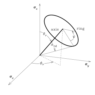
Figure 1: Geometry of the $r$th ring for the $d$th detector. The average direction of the spin axis over the $N_{\mathrm{s}}$ revolutions that make up the data on a single ring has polar angle $\theta_{r}$ and azimuth $\phi_{r}$, and is the same for all detectors. The ring opening angle $\alpha_{rd}$ depends on the detector and the ring (due to variation in the inertia tensor during the mission). For a given ring and detector, $\psi$ measures the angle around the ring. The point $\psi=0$ is defined as the most southerly intersection of the ring and the plane containing the ring axis and the $z$-direction. Note that $\psi=0$ is attained at different times for different detectors – the phase offsets being determined by the focal plane geometry.

2.3 The instrument response

We assume that the detector responses are linear functionals of the sky in the absence of instrument noise. At any instant, the power seen by a given detector (due to the sky) is given by convolving the sky with the appropriate beam and spectral transmission. A single time-ordered data point is then obtained by convolving this power with the detector’s temporal response.

2.3.1 Beam patterns

It is convenient to define the beam profile when the instrument is in the appropriate horn reference configuration, so that the beams can be assumed not to vary through the mission. A method for describing arbitrary, polarized beam patterns in terms of multipoles $b^{P}_{(lm)}$ was introduced by Challinor et al. [Challinor et al. 2000]. The beam pattern is first described in terms of effective Stokes parameters $\{\tilde{I}_{d}({\mn@boldsymbol{e}};\nu),\tilde{Q}_{d}({\mn@boldsymbol{e}};\nu),\tilde{U}_{d}({\mn@boldsymbol{e}};\nu),\tilde{V}_{d}({\mn@boldsymbol{e}};\nu)\}$, which are defined on the same $\{\mn@boldsymbol{\sigma}_{\theta},-\mn@boldsymbol{\sigma}_{\phi}\}$ basis as the sky. These effective Stokes parameters can be expressed in terms of the far-field radiation pattern of the detector [Challinor et al. 2000]. The $\tilde{Q}_{d}({\mn@boldsymbol{e}};\nu)$ and $\tilde{U}_{d}({\mn@boldsymbol{e}};\nu)$ can be combined into a linear polarization tensor for the beam, ${\mathcal{B}}_{d}^{ab}({\mn@boldsymbol{e}};\nu)$, as in equation (3). The resultant power per unit frequency interval, ${\mathrm{d}}W_{d}/{\mathrm{d}}\nu$, can then be written in basis-independent form as the integral

$$\frac{{\mathrm{d}}}{{\mathrm{d}}\nu}W_{d} = A_{{\mathrm{eff}},d}\int[I({\mn@boldsymbol{e}};\nu)\tilde{I}_{d}({\mn@boldsymbol{e}};\nu)-V({\mn@boldsymbol{e}};\nu)\tilde{V}_{d}({\mn@boldsymbol{e}};\nu)$$ (6)

$$\mbox{}+2{\mathcal{P}}_{ab}({\mn@boldsymbol{e}};\nu){\mathcal{B}}^{ab}_{d}({\mn@boldsymbol{e}};\nu)]\,{\mathrm{d}}\Omega,$$

where $A_{{\mathrm{eff}},d}$ is the effective area (assumed independent of frequency). The directivity $\tilde{I}_{d}({\mn@boldsymbol{e}};\nu)$ is a scalar field on the sphere, so can be expanded in terms of multipoles $b^{I}_{d(lm)}(\nu)$, as in equation (3). We impose the constraint $b^{I}_{d(00)}(\nu)=1/\sqrt{4\pi}$ so that $\tilde{I}_{d}({\mn@boldsymbol{e}};\nu)$ integrates to unity over the sphere. In a similar manner, $\tilde{V}_{d}({\mn@boldsymbol{e}};\nu)$ can be represented by multipoles $b^{V}_{d(lm)}(\nu)$. Finally, ${\mathcal{B}}^{ab}_{d}({\mn@boldsymbol{e}};\nu)$ can be expanded in the transverse, trace-free tensor harmonics with multipoles $b^{G}_{d(lm)}(\nu)$ and $b^{C}_{d(lm)}(\nu)$.

To obtain the power per unit frequency interval incident on the spectral filter chain for the $d$th detector, when the nominal main beam is at angle $\psi$ on the $r$th ring, we must rotate the beam pattern by $D(\phi_{r},\theta_{r},\psi)D(0,\alpha_{rd},\kappa_{rd})$ before performing the convolution in equation (6). This rotation is easily performed in multipole space to give the result [Challinor et al. 2000]

$$\frac{{\mathrm{d}}}{{\mathrm{d}}\nu}W_{rd}(\psi) = A_{{\mathrm{eff}},d}\sum_{Plmm^{\prime}m^{\prime\prime}}[a^{P\ast}_{(lm)}(\nu)\tilde{b}^{P}_{d(lm^{\prime})}(\nu)$$ (7)

$$\times D^{l}_{mm^{\prime\prime}}(\phi_{r},\theta_{r},\psi)D^{l}_{m^{\prime\prime}m^{\prime}}(0,\alpha_{rd},\kappa_{rd})],$$

where, for later convenience, we have defined

$$\tilde{b}^{P}_{d(lm)}(\nu) \equiv \delta_{I}^{P}b^{I}_{d(lm)}(\nu)-\delta^{P}_{V}b^{V}_{d(lm)}(\nu)$$ (8)

$$\mbox{}+2\delta_{G}^{P}b^{G}_{d(lm)}(\nu)+2\delta_{C}^{P}b^{C}_{d(lm)}(\nu),$$

with $b^{G}_{d(lm)}(\nu)=b^{C}_{d(lm)}(\nu)=0$ for $l<2$. The $D^{l}_{mm^{\prime}}(\alpha,\beta,\gamma)$ appearing in equation (7) are Wigner’s $D$-matrices; our conventions follow Brink & Satchler [Brink & Satchler 1993]. The dependence of $D^{l}_{mm^{\prime}}(\alpha,\beta,\gamma)$ on $\alpha$ and $\gamma$ goes as

$$D^{l}_{mm^{\prime}}(\alpha,\beta,\gamma)={\mathrm{e}}^{-im\alpha}d^{l}_{mm^{\prime}}(\beta){\mathrm{e}}^{-im^{\prime}\gamma},$$ (9)

where the $d^{l}_{mm^{\prime}}(\beta)$ are the reduced rotation matrices.

2.3.2 Spectral filtering

The power available at the detection element (e.g. bolometers for high frequency instruments) is given by integrating ${\mathrm{d}}W_{rd}(\psi)/{\mathrm{d}}\nu$ against the spectral transmission $v_{d}(\nu)$ of the filter chain. We shall assume that the filters on all detectors in a given frequency band are identical, and have transmission properties that are accurately known from calibrations on the ground. Map-making from multi-frequency data is usually performed on a band-by-band basis (although it is essential to use all the frequency bands to calibrate the pointing, e.g. van Leeuwen et al. 2001). Given that Fourier data from only detectors in the same frequency band are combined in such an analysis, we need only consider a single band, and henceforth assume that $v_{d}(\nu)$ has no dependence on the detector, i.e. $v_{d}(\nu)=v(\nu)$.

On integrating equation (7) against $v(\nu)$, the dependence on the sky enters through the integral $\int a^{P\ast}_{(lm)}(\nu)\tilde{b}^{P}_{d(lm^{\prime})}(\nu)v(\nu)\,{\mathrm{d}}\nu$. For the subsequent analysis, it is important that this integral can be factored into a part describing the sky carrying only $l$ and $m$ indices, and a part describing the beam which has only $l$ and $m^{\prime}$ indices. Here we assume that the approximate factorisation

$$\int a^{P\ast}_{(lm)}(\nu)\tilde{b}^{P}_{d(lm^{\prime})}(\nu)v(\nu)\,{\mathrm{d}}\nu \approx \tilde{b}^{P}_{d(lm^{\prime})}(\nu_{0})$$ (10)

$$\times\int a^{P\ast}_{(lm)}(\nu)v(\nu)\,{\mathrm{d}}\nu,$$

where $\nu_{0}$ is the central frequency in the band, is accurate to better than the noise level, so that we can describe the sky by the frequency integrated multipoles

$$\bar{a}^{P}_{(lm)}\equiv\int a^{P}_{(lm)}(\nu)v(\nu)\,{\mathrm{d}}\nu.$$ (11)

The largest source of error resulting from this factorisation is expected to be due to the variation of the width of the main beam across the band. In Appendix A we compute the systematic error on the recovered power spectrum of the CMB temperature anisotropies resulting from this variation, assuming an axisymmetric, diffraction-limited Gaussian beam, uniform sky coverage, and no foreground contaminants. For the Planck High Frequency Instrument (HFI), the bias may be non-negligible in the 100 GHz channel between $l=1000$ and $l=1500$, in which case refinements to equation (10) will be required. Here, we adopt the factorisation in equation (10), in which case the power available at the detection element, $W_{rd}(\psi)$, can be written as

$$W_{rd}(\psi) = A_{{\mathrm{eff}},d}\sum_{Plmm^{\prime}}[\bar{a}^{P\ast}_{(lm)}D^{l}_{mm^{\prime}}(\phi_{r},\theta_{r},\psi)$$ (12)

$$\phantom{A_{{\mathrm{eff}},d}\sum_{Plmm^{\prime}}}\times{\mathcal{B}}^{P}_{rd(lm^{\prime})}].$$

For later convenience, we have introduced the notation

$${\mathcal{B}}^{P}_{rd(lm^{\prime})}\equiv\sum_{m^{\prime\prime}}D^{l}_{m^{\prime}m^{\prime\prime}}(0,\alpha_{rd},\kappa_{rd})\tilde{b}^{P}_{d(lm^{\prime\prime})}(\nu_{0})$$ (13)

for the multipoles of the $d$th beam after rotation by $D(0,\alpha_{rd},\kappa_{rd})$. Note that the $r$-dependence of ${\mathcal{B}}^{P}_{rd(lm^{\prime})}$ derives only from the (slow) variation of opening angle $\alpha_{rd}$ and focal plane rotation $\kappa_{rd}$ through the mission.

2.3.3 Temporal response

The available power, $W_{rd}[\psi(t^{\prime})]$, is convolved with the temporal response function of the detector, $h_{d}(t,t^{\prime})$, to generate a single time-ordered datum at time $t$. We decompose $h_{d}(t,t^{\prime})$ into a stationary part, $h_{d}(t-t^{\prime})$, and a stochastic part, $\Delta h_{d}(t,t^{\prime})$, which we assume to have stationary statistical properties. The stochastic part, which derives from e.g. random fluctuations in amplifier gains, will be considered as part of the instrument noise in Section 2.4. Here, we concentrate on the stationary impulse response function $h_{d}(t)$. Typically, this will contain several instrument artifacts, such as the effect of finite sampling and non-zero detector time constants, which are convolved together to form the total impulse response. For example, if the detector time constant is $\tau_{d}$, and samples are taken by integrating over time intervals $\Delta_{d}$ and are assigned to the midpoint of the interval, then $h_{d}(t)=h_{\tau_{d},d}(t)\star h_{\Delta_{d},d}(t)$, where the detector impulse response

$$h_{\tau_{d},d}(t)=G_{d}\tau_{d}{}^{-1}{\mathrm{e}}^{-t/\tau_{d}}\Theta(t/\tau_{d}),$$ (14)

and the sampling impulse response

$$h_{\Delta_{d},d}(t)=\Delta_{d}{}^{-1}\Theta(1+2t/\Delta_{d})\Theta(1-2t/\Delta_{d}).$$ (15)

Here, $\Theta(x)$ is the Heaviside unit step function, and $G_{d}$ is the average gain over the mission, which includes both amplifier gain and the quantum efficiency of the detectors.

One of the advantages of describing the data on rings in the Fourier domain is that the convolution with the temporal response of the instrument reduces to a simple product [Delabrouille et al. 1998a]. Denoting the contribution of the signal to the phase-ordered data by $s_{rd}(\psi)$, we have

$$s_{rd}(\psi)=\int_{-\infty}^{\infty}W_{rd}(\psi+\omega_{r}t^{\prime})h_{d}(-t^{\prime})\,{\mathrm{d}}t^{\prime},$$ (16)

where $\omega_{r}={\mathrm{d}}\psi/{\mathrm{d}}t$ is the (average) spin rate on the $r$th ring. We have assumed that the support of $h_{d}(t)$ is sufficiently compact that the only contribution to $s_{rd}(\psi)$ is from the available power $W_{rd}$ on the same ring. We have further assumed that any variation of the spin rate about the average is negligible for the purpose of performing the convolution, so that the convolution of the available power with the impulse response is periodic in $\psi$. Inserting equation (12) into equation (16), and expanding $D^{l}_{mm^{\prime}}(\phi_{r},\theta_{r},\psi)$ as in equation (9), we find

$$s_{rd}(\psi) = A_{{\mathrm{eff}},d}\sum_{Plmm^{\prime}}[\bar{a}^{P\ast}_{(lm)}D^{l}_{mm^{\prime}}(\phi_{r},\theta_{r},\psi)$$ (17)

$$\phantom{A_{{\mathrm{eff}},d}\sum_{Plmm^{\prime}}}\times H_{d}^{\ast}(m^{\prime}\omega_{r}){\mathcal{B}}^{P}_{rd(lm^{\prime})}],$$

where $H_{d}(\omega_{r})$ is the Fourier transform of the impulse response:

$$H_{d}(\omega_{r})=\int_{-\infty}^{\infty}h_{d}(t){\mathrm{e}}^{-i\omega_{r}t}\,{\mathrm{d}}t.$$ (18)

For the impulse responses in equations (14) and (15), we have

$$H_{d}(\omega_{r})=\frac{G_{d}\,{\mathrm{sinc}}(\omega_{r}\Delta_{d}/2)}{1+i\omega_{r}\tau_{d}}.$$ (19)

Finally, we can extract from equation (17) the contribution of the signal to the $n$th Fourier coefficient of the phase-ordered data. Complex conjugating and using equation (9), we find

$$s_{(rdn)}=A_{{\mathrm{eff}},d}\sum_{Plm}[\bar{a}^{P}_{(lm)}d^{l}_{mn}(\theta_{r}){\mathrm{e}}^{im\phi_{r}}H_{d}(n\omega_{r}){\mathcal{B}}^{P\ast}_{rd(ln)}],$$ (20)

where the sum is over $l\geq|n|$ and $|m|\leq l$. Note that the effect of the impulse response can also be described in terms of an effective (ring-dependent) beam with multipoles

$$b^{P,{\mathrm{eff}}}_{rd(lm)}(\nu) = \sum_{m^{\prime}m^{\prime\prime}}[D^{l}_{mm^{\prime}}(-\kappa_{rd},-\alpha_{rd},0)H_{d}^{\ast}(m^{\prime}\omega_{r})$$ (21)

$$\phantom{\sum_{m^{\prime}m^{\prime\prime}}[}\times D^{l}_{m^{\prime}m^{\prime\prime}}(0,\alpha_{rd},\kappa_{rd})b^{P}_{d(lm^{\prime\prime})}(\nu)].$$

The effective beam will be generally not be axisymmetric as a consequence of the smearing along the scan direction induced by the impulse response of the instrument. The concept of an effective beam becomes particularly significant if the beam has to be calibrated from the observations of e.g. bright point source transits, as described by van Leeuwen et al. [van Leeuwen et al. 2001]. In such cases, it is the effective beam that can be reconstructed most directly. A potential difficulty that would need to be addressed in such an approach is the (slow) variation of effective beam with ring due to variations in the angles $\alpha_{rd}$ and $\kappa_{rd}$. In practice, it may be simpler to deconvolve the temporal response of the instrument prior to construction of the phase-ordered data. In this case, $H_{d}(n\omega_{r})$ can be omitted from equation (20).

2.4 Gaussian random noise and reconstruction errors

The Fourier modes, $t_{(rdn)}$, that we construct from the phase-ordered data differ from the $s_{(rdn)}$ of equation (20) because of a number of sources of error. For example, stochasticity in the instrument temporal response, such as that due to thermal noise in the detectors and amplifiers, has not been included in equation (20). Neither have we included the effects of photon (shot) noise, or any detector offsets. Furthermore, we have replaced the spin axis pointing by its average over the $N_{\mathrm{s}}$ spin periods, ignoring the (albeit small) effects of the nutation of the instrument. These random errors tend to be suppressed in the phase-ordered data due to the averaging over $N_{\mathrm{s}}$ periods, except for fluctuations at temporal frequencies synchronous with the spin frequency. Fluctuations below the spin frequency remain in the phase-ordered data predominantly as an offset on the ring. In the usual map-making paradigm [Bond et al. 1999, Borrill 1999], low frequency ($1/f$) noise must be carefully accounted for; failure to do so leads to highly correlated errors in the reconstructed map which typically appear as stripes (e.g. Delabrouille 1998; Revenu et al. 2000). It is difficult to accommodate low frequency noise power in map-making from the time-ordered data since its inclusion spoils the sparse nature of the time-time noise correlation matrix. Approximate methods to circumvent this problem for experiments that scan on rings already exist [Delabrouille 1998, Revenu et al. 2000]; these ‘destriping’ methods will be discussed further in Section 4.1.

There are also a number of potential systematic errors which contaminate the $t_{(rdn)}$, and, if left unaccounted for, will lead to bias in the reconstructed multipoles of the sky. Keeping the numerous systematics under control is essential to maintaining the integrity of the final data products. A significant merit of the harmonic data model is that the model of the instrument, equation (20), is sufficiently complete to include a number of systematic effects which are not so naturally included in the standard map-making techniques. For example, the harmonic model can seamlessly accommodate any prior knowledge we have of asymmetries in the beam profiles, cross-polar contamination for the polarized detectors, sidelobe features leading to ‘straylight’ entering the instrument, and detector time constants and data sampling rate. For some systematics there will be incomplete (or even no) prior knowledge of essential parameters, in which case these parameters must be estimated from the data themselves during the reconstruction of the sky. The harmonic model also appears well-suited to handling such systematics iteratively; see Section 4.2.

To include the effect of Gaussian random noise with a known (or estimated) power spectrum in the reconstruction of the sky from the Fourier data on rings, $t_{(rdn)}$, we require the covariance matrix $N_{(rdn)(r^{\prime}d^{\prime}n^{\prime})}$. This matrix was calculated by Delabrouille at al. [Delabrouille et al. 1998a] for a single detector and ring ($d=d^{\prime}$ and $r=r^{\prime}$). Here we extend their result to include the effects of a finite sampling rate (see also Janssen et al. 1996), and to allow for $r\neq r^{\prime}$. Assuming instrument noise dominates the random errors $\Delta t_{(rdn)}$, there will be negligible correlation between the errors on different detectors, so we need only consider $d=d^{\prime}$.

We assume that the noise contribution, $n_{d}(t)$, to the time stream of the $d$th detector is a real, stationary random process with zero mean, and power spectrum ${\mathcal{N}}_{d}(\omega)$. The power spectrum is the Fourier transform of the noise auto-correlation function $C_{d}(\tau)=\langle n_{d}(t+\tau)n_{d}(t)\rangle$:

$${\mathcal{N}}_{d}(\omega)=\int_{-\infty}^{\infty}C_{d}(\tau){\mathrm{e}}^{-i\omega\tau}\,{\mathrm{d}}\tau.$$ (22)

The propagation of the noise $n_{d}(t)$ to the errors $\Delta t_{(rdn)}$ depends on the exact procedure for estimating the Fourier modes $t_{(rdn)}$ from the time-ordered data [van Leeuwen et al. 2001]. However, to a first approximation, the errors $\Delta t_{(rdn)}$ are obtained by convolving $n_{d}(t)$ with the impulse response of the sampler, $h_{\Delta_{d},d}(t)$, mapping the portion of this function covering the observation interval for the $r$th ring onto the angle $\psi$ around the ring, and finally extracting the Fourier coefficients of the resultant signal:

$$\Delta t_{(rdn)}=\frac{\omega_{r}}{2\pi}\int_{t_{rd}^{-}}^{t_{rd}^{+}}h_{\Delta_{d},d}\star n_{d}(t)\exp[-in\omega_{r}(t-t_{rd}^{-})]\,{\mathrm{d}}t.$$ (23)

Here, $t_{rd}^{-}$ is the time when the $d$th detector is first pointing to $\psi=0$ on the $r$th ring, $t_{rd}^{+}$ is the end of the observation interval for that ring: $t_{rd}^{+}=t_{rd}^{-}+2\pi N_{\mathrm{s}}/\omega_{r}$, and we have ignored any variation of the spin rate during the $N_{\mathrm{s}}$ revolutions. It is now straightforward to write the covariance of the errors in terms of the noise power spectrum. For the case of scanning missions such as Planck, the number of revolutions $N_{\mathrm{s}}\gg 1$ is sufficiently large that negligible correlations remain between different Fourier modes. In this case we find

$$N_{(rdn)(r^{\prime}d^{\prime}n^{\prime})} = \delta_{dd^{\prime}}\delta_{nn^{\prime}}\frac{1}{2\pi}\int_{-\infty}^{\infty}\{{\mathcal{N}}_{d}(\omega){\mathrm{sinc}}^{2}(\omega\Delta_{d}/2)$$ (24)

$$\mbox{}\times{\mathrm{sinc}}^{2}[(\omega/\omega_{r}-n)\pi N_{{\mathrm{s}}}]$$

$$\mbox{}\times\exp[i2\pi N_{\mathrm{s}}(r-r^{\prime})\omega/\omega_{r}]\}\,{\mathrm{d}}\omega,$$

where we have further ignored any variation of the average spin rate, $\omega_{r}$, between rings. Provided that ${\mathcal{N}}_{d}(\omega){\mathrm{sinc}}^{2}(\omega\Delta_{d}/2)$ varies slowly compared to the rest of the integrand in equation (24) around $\omega=n\omega_{r}$, we can replace it by its value there. The remaining integral vanishes unless $r=r^{\prime}$, so that for slowly varying power spectra the covariance matrix is fully diagonal:

$$N_{(rdn)(r^{\prime}d^{\prime}n^{\prime})} = \delta_{rr^{\prime}}\delta_{dd^{\prime}}\delta_{nn^{\prime}}$$ (25)

$$\mbox{}\times\frac{\omega_{r}}{2\pi N_{\mathrm{s}}}{\mathcal{N}}_{d}(n\omega_{r}){\mathrm{sinc}}^{2}(n\omega_{r}\Delta_{d}/2).$$

In the presence of a significant low frequency noise component (such as $1/f$ noise in the electronics) joining onto white noise at a knee frequency $\omega_{\mathrm{knee}}$ (e.g. Delabrouille 1998), the assumption of a slowly varying noise power spectrum may not hold for small $|n|$. Typically the spin rate will be chosen so that $\omega_{\mathrm{knee}}\ll\omega_{r}$, in which case equation (25) will be valid for $n\neq 0$. However, for $n=0$ we can expect correlations between rings unless $\omega_{r}/N_{{\mathrm{s}}}\ll\omega_{\mathrm{knee}}\ll\omega_{r}$. (For the Planck HFI, the nominal $\omega_{\mathrm{knee}}<0.06\,{\mathrm{rad}}\,{\mathrm{s}}^{-1}$, and $\omega_{r}\approx 0.10\,{\mathrm{rad}}\,{\mathrm{s}}^{-1}$, so these conditions are likely to be satisfied.) Even in the presence of such correlations, the noise covariance matrix is still block diagonal in the harmonic representation, in contrast to the time-time covariance matrix which has significant off-diagonal terms due to the extended support of the noise auto-correlation function, $C_{d}(\tau)$.

2.5 Maximum-likelihood solution

Our model for the ring Fourier data $t_{(rdn)}$ is now $t_{(rdn)}=s_{(rdn)}+\Delta t_{(rdn)}$, where the signal $s_{(rdn)}$ is modelled by equation (20). It is convenient to write this relation in the form

$$t_{(rdn)}=\sum_{Plm}A_{(rdn)(Plm)}\bar{a}^{P}_{(lm)}+\Delta t_{(rdn)},$$ (26)

where the coupling matrix is

$$A_{(rdn)(Plm)}\equiv A_{{\mathrm{eff}},d}d^{l}_{mn}(\theta_{r}){\mathrm{e}}^{im\phi_{r}}H_{d}(n\omega_{r}){\mathcal{B}}^{P\ast}_{rd(ln)}.$$ (27)

We define $A_{(rdn)(Plm)}$ to be zero for $l<|n|$, since the $t_{(rdn)}$ only depend on the $\bar{a}^{P}_{(lm)}$ with $l\geq|n|$. This structure can be exploited to derive an unbiased (although not minimal variance) estimator for the $\bar{a}^{P}_{(lm)}$, which can be computed in $O(l_{\mathrm{max}}^{4})$ operations. Here, $l_{\mathrm{max}}$ is the maximum $l$ that we retain during the inversion. (The experimental beam limits $l_{\mathrm{max}}$ even if the underlying sky is not band-limited.) The estimate is derived by working down from the maximum Fourier mode, $n_{\mathrm{max}}$, and performing a regularised inversion of a subset of the data to solve for those $\bar{a}^{P}_{(lm)}$ on which the data subset depends but which have not been determined at a previous step. Full details of this estimator will be given in a future paper (Mortlock et al. in preparation).

In this paper we shall just give the formal maximum-likelihood solution to equation (26). We assume that we are attempting to solve only for the $\bar{a}^{P}_{(lm)}$ which form the components of a vector $\mn@boldsymbol{a}$. In practice, it may also be desirable to attempt to solve for several instrument parameters which are unknown from earlier calibrations, but which represent significant systematic effects. Such parameters are easily included in the maximum-likelihood formalism, but unless they influence the data linearly their inclusion would prevent us from being able to locate the maximum-likelihood multipoles analytically. Given the size of the problem, having to locate the maximum of the likelihood by a numerical search in model space is clearly undesirable. The treatment of systematics with unknown parameters is probably best performed iteratively (e.g. Delabrouille, Gispert & Puget 1998b; see also Section 4.2).

Assuming Gaussian noise, the maximum-likelihood estimate, $\hat{\mn@boldsymbol{a}}$, for the true sky, $\mn@boldsymbol{a}$, is

$$\hat{\mn@boldsymbol{a}}=({\textbf{{A}}}^{\dagger}{\textbf{{N}}}^{-1}{\textbf{{A}}})^{-1}{\textbf{{A}}}^{\dagger}{\textbf{{N}}}^{-1}\mn@boldsymbol{t},$$ (28)

where $\mn@boldsymbol{t}$ is the vector of Fourier modes $t_{(rdn)}$, A is the matrix of coupling coefficients $A_{(rdn)(r^{\prime}d^{\prime}n^{\prime})}$, and N is the noise covariance matrix with components $N_{(rdn)(r^{\prime}d^{\prime}n^{\prime})}$. The ^† operation in equation (28) denotes Hermitian conjugation. The maximum-likelihood solution is the optimal, unbiased estimate of the sky. Its covariance matrix is

$${\textbf{{C}}}\equiv\langle(\hat{\mn@boldsymbol{a}}-\mn@boldsymbol{a})(\hat{\mn@boldsymbol{a}}-\mn@boldsymbol{a})^{\dagger}\rangle=({\textbf{{A}}}^{\dagger}{\textbf{{N}}}^{-1}{\textbf{{A}}})^{-1},$$ (29)

where the average is over noise realisations. A brute force evaluation of $\hat{\mn@boldsymbol{a}}$ requires $O(l_{\mathrm{max}}^{6})$ operations and $O(l_{\mathrm{max}}^{4})$ storage which is impossible at the moment for high resolution experiments. Conjugate gradient techniques (e.g. Press et al. 1992) would reduce the operations count to $O(N_{\mathrm{i}}l_{\mathrm{max}}^{4})$, where $N_{\mathrm{i}}$ is the number of iterations required, by removing the matrix multiplies and inversion. Note that the block-diagonal structure of N (equation 24) reduces the cost of computing $\textbf{{N}}^{-1}$ to $O(l_{\mathrm{max}}^{4})$ operations, or fewer if correlations between rings are confined to the $n=0$ modes. Keeping $N_{\mathrm{i}}$ small requires a careful choice of preconditioner, i.e. a Hermitian, positive-definite matrix which is both a good approximation to the inverse covariance matrix ${\textbf{{C}}}^{-1}$ and is easy to invert. We demonstrate in Section 3 that for simple scan strategies such matrices can easily be found (see also Oh et al. 1999). For the case where all rings are at similar latitude, an approximation to ${\textbf{{C}}}^{-1}$ can be computed in $O(l_{\mathrm{max}}^{4})$ operations and requires only $O(l_{\mathrm{max}}^{3})$ storage. This preconditioner is block-diagonal and can be inverted in $O(l_{\mathrm{max}}^{4})$ operations. Note, however, that the conjugate gradient evaluation of equation (29) still requires $O(l_{\mathrm{max}}^{4})$ storage for the non-sparse matrix A. The application of the conjugate gradient method, as well other iterative techniques, to equation (29) will be explored numerically in Mortlock et al. (in preparation).

In writing down the maximum-likelihood solution we have assumed that ${\textbf{{A}}}^{\dagger}{\textbf{{N}}}^{-1}\textbf{{A}}$ is invertible, so that the solution is unique. For some scan strategies and instrument geometries, ${\textbf{{A}}}^{\dagger}{\textbf{{N}}}^{-1}{\textbf{{A}}}$ may become numerically singular due to incomplete coverage of the sky. With incomplete coverage, and $l_{\mathrm{max}}$ sufficiently large, there may exist sets of multipoles which produce a temperature or polarization field which is localised to machine precision in the regions of the sky that are not covered [Mortlock et al. 2001]. In such cases, solving for the multipoles must proceed via singular value techniques, and we obtain no constraint on the part of $\mn@boldsymbol{a}$ which lies in the null space of the coupling matrix A. If map-making were performed in pixel space, similar problems would arise when attempting to estimate the multipoles from the pixelised map. As an alternative to singular-value techniques, we could further regularise the inversion by Wiener filtering. With a Gaussian prior for the signal $\mn@boldsymbol{a}$, with covariance ${\textbf{{S}}}\equiv\langle\mn@boldsymbol{a}\mn@boldsymbol{a}^{\dagger}\rangle$, the maximum of the posterior probability gives the Wiener-filtered reconstruction

$$\hat{{\mn@boldsymbol{a}}}=({\textbf{{S}}}^{-1}+{\textbf{{A}}}^{\dagger}{\textbf{{N}}}^{-1}{\textbf{{A}}})^{-1}{\textbf{{A}}}^{\dagger}{\textbf{{N}}}^{-1}{\mn@boldsymbol{t}}.$$ (30)

In this manner, the inversion of the singular matrix ${\textbf{{A}}}^{\dagger}{\textbf{{N}}}^{-1}{\textbf{{A}}}$ is regularised by the inverse signal covariance matrix ${\textbf{{S}}}^{-1}$. In practice, the microwave sky is only poorly approximated as a Gaussian random process, particularly in those frequency channels where the CMB is not dominant. In addition, we will only have limited knowledge of the signal covariance matrix S either from other observations, or a preliminary, approximate analysis of the data. However, Wiener filtering has proved to be a useful technique in component separation where similar objections to the use of Gaussian priors hold (see e.g. Hobson et al. 1998 and references therein), and the same should be true for harmonic ‘map’-making. Note that Wiener filtering produces a biased estimate of the sky; other linear filters have been proposed to cirumvent this problem, but generally produce noisier, though unbiased, maps (e.g. Tegmark & Efstathiou 1996). Equation (30) can also be solved with conjugate gradient techniques; in this case the preconditioner should include some simplified form of the signal covariance in addition to an approximation to ${\textbf{{A}}}^{\dagger}{\textbf{{N}}}^{-1}{\textbf{{A}}}$ .

In our discussion so far we have assumed that full beam deconvolution is performed during the ‘map’-making stage. In practice, deconvolving the beam completely may be undesirable for several reasons. Firstly, the matrix ${\textbf{{A}}}^{\dagger}{\textbf{{N}}}^{-1}{\textbf{{A}}}$ is likely to be more ill-conditioned since the errors on the reconstructed multipoles must grow large as $l$ approaches the (inverse) beam scale. (In a conjugate gradients solution, the preconditioner can partly take this effect into account.) Secondly, as discussed in Section 2.3.2 and Appendix A, variation of the width of the main beam across the spectral band of a channel is a potential source of systematic error. For an asymmetric beam, one could make the optimistic assumption beam multipoles in a given frequency channel could be written as the product of a frequency-dependent, symmetric part $\tilde{b}^{P}_{(l0)}(\nu)$ which is assumed to be the same for all detectors in the band, and a frequency-independent, asymmetric part which may depend on the detector:

$$\tilde{b}^{P}_{d(lm)}(\nu)\approx\tilde{b}^{P}_{(l0)}(\nu)[\tilde{b}^{P}_{d(lm)}(\nu_{0})/\tilde{b}^{P}_{(l0)}(\nu_{0})],$$ (31)

where $\nu_{0}$ is the central frequency in the band. We could then solve for the multipoles of the sky convolved with an effective symmetric beam with multipoles $\tilde{b}^{P}_{(lm)}(\nu)$ and integrated across the frequency band with filter $v(\nu)$. By factoring the beam in this way, we can simultaneously improve the condition number of ${\textbf{{A}}}^{\dagger}{\textbf{{N}}}^{-1}{\textbf{{A}}}$ and remove most of the bias due to variation of the main beam width with frequency.

3 Simple scan strategies

In this section we investigate the structure of the inverse covariance matrix, $\textbf{{C}}^{-1}$, of the recovered multipoles for two simple scanning strategies. The first is a random pointing of the spin axis for each ring, which ensures uniform coverage of the entire sky. The second is constant latitude scanning, where all rings have the same polar angle, $\theta_{r}=\theta$. Constant latitude scanning is a useful approximation to the scan strategy of the Planck satellite, where the spin axis stays close to the plane of the ecliptic. By adopting coarse restrictions on the behaviour of the instrument, we are able to demonstrate that, under these restrictions, the harmonic estimate of the sky, equation (28), is statistically equivalent to that obtained via conventional map-making and spherical analysis. By relaxing some restrictions on the behaviour of the instrument, we obtain some useful extensions of the known results.

Throughout this section we impose a number of limits on the instrument response: (i) The spin axis position is always aligned with the $z$-axis of the instrument reference system (see Section 2.2), so that the ring opening angles, $\alpha_{rd}$, are independent of $r$, and the focal plane rotations $\kappa_{rd}=0$; (ii) There is no variation in average spin rate between rings, so we can drop the subscript from $\omega_{r}$; (iii) The band width of the spectral filters is sufficiently narrow that

$$\int a^{P\ast}_{(lm)}(\nu)\tilde{b}^{P}_{(lm^{\prime})}(\nu)v(\nu)\,{\mathrm{d}}\nu = a^{P\ast}_{(lm)}(\nu_{0})\tilde{b}^{P}_{(lm^{\prime})}(\nu_{0})$$ (32)

$$\mbox{}\times\int v(\nu)\,{\mathrm{d}}\nu,$$

where $\nu_{0}$ is the central frequency of the band; (iv) Bolometer time constants, $\tau_{d}$, and the sampling period, $\Delta_{d}$, are such that $\tau_{d}\omega_{r}l_{\mathrm{max}}\ll 1$ and $\Delta_{d}\omega_{r}l_{\mathrm{max}}\ll 1$, in which case the effect of the instrument response can be approximated by simply a gain at zero lag; (v) The noise power spectrum is white so that

$$N_{(rdn)(r^{\prime}d^{\prime}n^{\prime})}=\delta_{rr^{\prime}}\delta_{dd^{\prime}}\delta_{nn^{\prime}}\sigma_{d}^{2},$$ (33)

where $\sigma^{2}_{d}$ is a constant for each detector, which can be related to the detector sensitivity, $s_{d}$. With the restrictions above,

$$s_{d} = \left[A_{{\mathrm{eff}},d}G_{d}\bar{T}\left.\frac{\partial B(\nu_{0},T)}{\partial T}\right|_{T=\bar{T}}\int v(\nu)\,{\mathrm{d}}\nu\right]^{-1}$$ (34)

$$\mbox{}\times\sqrt{\frac{2\pi N_{\mathrm{s}}}{\omega_{r}}}\sigma_{d},$$

where $B(\nu,T)$ is the Planck function and the average CMB temperature is $\bar{T}$. Note that a consequence of restriction (i) is that ${\mathcal{B}}^{P}_{rd(ln)}$ is independent of ring, ${\mathcal{B}}^{P}_{rd(ln)}={\mathcal{B}}^{P}_{d(ln)}$. If we define dimensionless multipoles by

$$\tilde{a}^{P}_{(lm)}\equiv\left[\bar{T}\left.\frac{\partial B(\nu_{0},T)}{\partial T}\right|_{T=\bar{T}}\right]^{-1}a^{P}_{(lm)}(\nu_{0}),$$ (35)

the inverse of the dimensionless error covariance matrix, $\tilde{\textbf{{C}}}^{-1}$, has components

$$\tilde{C}^{-1}_{(Plm)(P^{\prime}l^{\prime}m^{\prime})} = \frac{2\pi N_{\mathrm{s}}}{\omega}\sum_{rdn}s_{d}^{-2}\{D^{l}_{mn}(\phi_{r},\theta_{r},0){\mathcal{B}}^{P}_{d(ln)}$$ (36)

$$\mbox{}\times[D^{l^{\prime}}_{m^{\prime}n}(\phi_{r},\theta_{r},0){\mathcal{B}}^{P^{\prime}}_{d(l^{\prime}n)}]^{\ast}\},$$

where the sum is over detectors, rings, and $|n|\leq{\mathrm{min}}(l,l^{\prime})$. We now proceed to analyse $\tilde{\textbf{{C}}}^{-1}$ for randomly-positioned rings and constant latitude scanning.

3.1 Randomly-positioned rings

We consider the limit of equation (36) as the number of rings $N_{\mathrm{r}}\rightarrow\infty$ while keeping the survey length finite, in which case we can replace the sum over rings by an appropriate integral. In practice, for finite $N_{\mathrm{r}}$ the continuum limit should hold for scales with $l\la\sqrt{N_{\mathrm{r}}/(4\pi)}$. Placing the rings at random is equivalent to enforcing uniform coverage of the full sky, which will allow us to make contact with existing analytic results obtained from the map-based formalism. The sum over randomly-positioned rings in equation (36) can be replaced by $[N_{\mathrm{r}}/(4\pi)]\int\,{\mathrm{d}}\Omega_{r}$, where ${\mathrm{d}}\Omega_{r}\equiv{\mathrm{d}}\phi_{r}\,{\mathrm{d}}\cos\theta_{r}$. Making use of the orthogonality of the $D^{l}_{mm^{\prime}}(\alpha,\beta,\gamma)$ over the ${\mathrm{SO}}(3)$ group manifold [Brink & Satchler 1993], we find

$$\int D^{l}_{mn}(\phi_{r},\theta_{r},0)[D^{l^{\prime}}_{m^{\prime}n}(\phi_{r},\theta_{r},0)]^{\ast}\,{\mathrm{d}}\Omega_{r}=\frac{4\pi}{2l+1}\delta_{ll^{\prime}}\delta_{mm^{\prime}},$$ (37)

so that $\tilde{\textbf{{C}}}^{-1}$ simplifies to

$$\tilde{C}^{-1}_{(Plm)(P^{\prime}l^{\prime}m^{\prime})}=\delta_{ll^{\prime}}\delta_{mm^{\prime}}\frac{T_{\mathrm{m}}}{2l+1}\sum_{dn}s_{d}^{-2}{\mathcal{B}}^{P}_{d(ln)}{\mathcal{B}}^{P^{\prime}\ast}_{d(ln)},$$ (38)

where the total mission time is $T_{\mathrm{m}}=2\pi N_{\mathrm{s}}N_{\mathrm{r}}/\omega$. Equation (38) can be further simplified by using equation (13) to substitute for ${\mathcal{B}}^{P}_{d(ln)}$ and then performing the sum over $n$ noting that $[D^{l}_{mn}(\alpha,\beta,\gamma)]^{\ast}=D^{l}_{nm}(-\gamma,-\beta,-\alpha)$. The result is

$$\tilde{C}^{-1}_{(Plm)(P^{\prime}l^{\prime}m^{\prime})} = \delta_{ll^{\prime}}\delta_{mm^{\prime}}\frac{T_{\mathrm{m}}}{2l+1}$$ (39)

$$\mbox{}\times\sum_{dm^{\prime\prime}}s_{d}^{-2}\tilde{b}^{P}_{d(lm^{\prime\prime})}(\nu_{0})\tilde{b}^{P^{\prime}\ast}_{d(lm^{\prime\prime})}(\nu_{0}).$$

Note that there is now no dependence on the opening angles of the detectors, $\alpha_{rd}=\alpha_{d}$. This is a consequence of assuming white noise. If the noise had a characteristic timescale, this would combine with the spin velocity and opening angle to define a characteristic angular scale for the projected noise, and $\tilde{\textbf{{C}}}$ would then depend on $\alpha_{d}$.

To make further progress, we consider initially the case where the beams are axisymmetric, and have no cross-polar contamination. In this limit, the intensity multipoles can be written in terms of a window function, $W_{l,d}$:

$$b^{I}_{d(lm)}(\nu_{0})=\sqrt{\frac{2l+1}{4\pi}}W_{l,d}\delta_{m0},$$ (40)

and the linear polarization multipoles in terms of spin-weight 2 window functions, ${}_{2}W_{l,d}$, (Challinor et al. 2000; see also Ng & Liu 1999):

$$b^{G}_{d(lm)}(\nu_{0}) = -\sqrt{\frac{2l+1}{32\pi}}{}_{2}W_{l,d}{\mathrm{e}}^{-im\rho_{d}}(\delta_{m2}+\delta_{m\,-2}),$$ (41)

$$b^{C}_{d(lm)}(\nu_{0}) = -i\sqrt{\frac{2l+1}{32\pi}}{}_{2}W_{l,d}{\mathrm{e}}^{-im\rho_{d}}(\delta_{m2}-\delta_{m\,-2}).$$ (42)

Here, $\rho_{d}$ is the angle between the polarization direction on axis and the normal to the plane containing the main beam direction and the spin axis. (The unit normal to this plane is $\mn@boldsymbol{\sigma}_{y}$ when the detector is in its horn’s reference configuration). By assumption, the circular polarization multipoles for the beam vanish. Substituting into equation (39), we find

$$\tilde{C}^{-1}_{(Plm)(P^{\prime}l^{\prime}m^{\prime})} = \delta_{ll^{\prime}}\delta_{mm^{\prime}}\delta_{PP^{\prime}}$$ (43)

$$\times\sum_{d}w_{d}[\delta^{P}_{I}W_{l,d}^{2}+(\delta^{P}_{G}+\delta^{P}_{C}){}_{2}W_{l,d}^{2}],$$

where we have introduced the weight per solid angle [Knox 1995], which for uniform coverage of the sky is $w_{d}\equiv T_{\mathrm{m}}/(4\pi s_{d}^{2})$. Note that the covariance matrix is diagonal, and that it does not depend on the relative orientations of the polarization directions of the various detectors. This is not surprising since for randomly-positioned rings, every point on the sky is traversed by every detector in every possible orientation, and we have assumed the instrument noise to be uncorrelated between detectors.

It is straightforward to show that the covariance matrix in equation (43) is equal to that obtained by constructing optimal (minimum variance), beam-smoothed maps of the Stokes parameters for each detector, and then optimally extracting the $\tilde{a}^{P}_{(lm)}$ from a joint analysis of the maps. If the main beam of the $d$th detector lies in the $p$th pixel when the ring phase is $\psi$ on the $r$th ring, the signal contribution to the phase-ordered data, equation (17), can be written as (see e.g. Challinor et al. 2000)

$$s_{rd}(\psi) = A_{{\mathrm{eff}},d}G_{d}\bar{T}\left.\frac{\partial B(\nu_{0},T)}{\partial T}\right|_{T=\bar{T}}\int v(\nu)\,{\mathrm{d}}\nu[I_{{\mathrm{eff}},d}({\mn@boldsymbol{e}}_{p})$$ (44)

$$\mbox{}-Q_{{\mathrm{eff}},d}({\mn@boldsymbol{e}}_{p})\cos 2\eta+U_{{\mathrm{eff}},d}({\mn@boldsymbol{e}}_{p})\sin 2\eta].$$

under the restrictions described above. In equation (44), ${\mn@boldsymbol{e}}_{p}$ is in the direction of the $p$th pixel, and has polar angle $\theta_{p}$ and azimuth $\phi_{p}$, and the angle $\eta$ is the angle between the polarization direction (on the sky) along the beam axis and the plane containing ${\mn@boldsymbol{e}}_{p}$ and the $z$-axis of the fixed reference system. The beam-smoothed fields are

$$I_{{\mathrm{eff}},d}({\mn@boldsymbol{e}}) = \sum_{lm}W_{l,d}\tilde{a}^{I}_{(lm)}Y_{(lm)}({\mn@boldsymbol{e}})$$ (45)

$$\frac{1}{\sqrt{2}}(Q_{{\mathrm{eff}},d}\pm iU_{{\mathrm{eff}},d})({\mn@boldsymbol{e}}) = \sum_{lm}[{}_{2}W_{l,d}(\tilde{a}^{G}_{(lm)}\mp i\tilde{a}^{C}_{(lm)})$$ (46)

$$\mbox{}\times{}_{\mp 2}Y_{(lm)}({\mn@boldsymbol{e}})],$$

where the ${}_{\pm 2}Y_{(lm)}$ are examples of the spin-weight harmonics, defined for integer $s$ by [Goldberg et al. 1967]

$$D^{l}_{m\,-s}(\alpha,\beta,\gamma)=(-1)^{s}\sqrt{\frac{4\pi}{2l+1}}{}_{s}Y^{\ast}_{(lm)}(\beta,\alpha){\mathrm{e}}^{is\gamma}.$$ (47)

For randomly-positioned rings in the limit $N_{\mathrm{r}}\rightarrow\infty$, the angles $\psi$ are uniformly covered in any given pixel. Given our assumptions, the optimal, unbiased estimate for $I_{{\mathrm{eff}},d}$ in the $p$th pixel is given by direct averaging of the appropriate $t_{rd}(\psi)$. For $Q_{{\mathrm{eff}},d}$ the $t_{rd}(\psi)$ are averaged with weight $-2\cos 2\eta$, and for $U_{{\mathrm{eff}},d}$ the weight is $2\sin 2\eta$. The errors on the smoothed maps are uncorrelated between Stokes parameters, and between pixels. The errors on these maps have weights per solid angle $w_{d}$ for $I_{{\mathrm{eff}},d}$, and $w_{d}/2$ for $Q_{{\mathrm{eff}},d}$ and $U_{{\mathrm{eff}},d}$.

For uncorrelated noise between Stokes parameters, pixels, and detectors, the maximum-likelihood estimate of the $\tilde{a}^{P}_{(lm)}$ from the smoothed maps reduces to minimising the (absolute) squared residuals between the left and right-hand sides of equations (45) and (46), with each pixel for each detector entering with the appropriate weight per solid angle. In the case of uniform coverage considered in this subsection, the maximum-likelihood estimates of the $\tilde{a}^{P}_{(lm)}$ are equivalent to performing a spherical transform of the smoothed maps and then averaging these across the detectors, with each detector carrying statistical weight $W_{l,d}w_{d}$. However, it will be useful for the next subsection to note the form that the error covariance matrix takes when we relax the assumption of uniform coverage, while retaining the assumptions of uncorrelated errors between Stokes parameters, detectors and pixels. The weights per solid angle for $I_{{\mathrm{eff}},d}$ are then pixel-dependent, $w_{d,p}$, and the weights for $Q_{{\mathrm{eff}},d}$ and $U_{{\mathrm{eff}},d}$ are $w_{d,p}/2$. The non-vanishing entries of the inverse of the (Hermitian) error covariance matrix are then:

$$\tilde{C}^{-1}_{(Ilm)(Il^{\prime}m^{\prime})} = \sum_{pd}W_{l,d}W_{l^{\prime},d}w_{d,p}Y_{(lm)}^{\ast}Y_{(l^{\prime}m^{\prime})}\Delta\Omega_{p},$$ (48)

$$\tilde{C}^{-1}_{(Glm)(Gl^{\prime}m^{\prime})} = \sum_{pd}[{}_{2}W_{l,d}\,{}_{2}W_{l^{\prime},d}w_{d,p}{\textstyle{\frac{1}{2}}}({}_{2}Y_{(lm)}^{\ast}{}_{2}Y_{(l^{\prime}m^{\prime})}$$ (49)

$$\phantom{\sum_{pd}}+{}_{-2}Y_{(lm)}^{\ast}{}_{-2}Y_{(l^{\prime}m^{\prime})})\Delta\Omega_{p}],$$

$$\tilde{C}^{-1}_{(Glm)(Cl^{\prime}m^{\prime})} = i\sum_{pd}[{}_{2}W_{l,d}\,{}_{2}W_{l^{\prime},d}w_{d,p}{\textstyle{\frac{1}{2}}}({}_{2}Y_{(lm)}^{\ast}{}_{2}Y_{(l^{\prime}m^{\prime})}$$ (50)

$$\phantom{\sum_{pd}}-{}_{-2}Y_{(lm)}^{\ast}{}_{-2}Y_{(l^{\prime}m^{\prime})})\Delta\Omega_{p}],$$

and $\tilde{C}^{-1}_{(Clm)(Cl^{\prime}m^{\prime})}=\tilde{C}^{-1}_{(Glm)(Gl^{\prime}m^{\prime})}$. Here, $\Delta\Omega_{p}$ is the solid angle subtended by the $p$th pixel. For the case of uniform coverage, $w_{d,p}=w_{d}$, the orthonormality of the spin-weight harmonics reduces equations (48)–(50) to the result derived from the harmonic model, equation (43), if we ignore pixelisation effects. For this simple example, the estimates of the $a^{P}_{(lm)}$ from the harmonic model and the map-making route are both unbiased and have the same error covariance. It follows that they are statistically equivalent at the level of second-order correlations (and at all orders for Gaussian noise).

3.1.1 Effect of beam asymmetry

We now consider the effect of a known beam asymmetry on the covariance matrices obtained via the harmonic and map-based routes. For simplicity, we shall only consider unpolarized detectors with bivariate Gaussian profiles, with eccentricity $e_{d}$. Consider initially a detector in its horn’s reference configuration, with the major axis of the iso-directivity ellipse aligned with $\mn@boldsymbol{\sigma}_{x}$. For beam widths $\sigma_{d}\ll 1$, we have

$$\tilde{I}_{d}({\mn@boldsymbol{e}};\nu_{0})\approx\frac{\exp\{-\theta^{2}[\cos^{2}\phi+\sin^{2}\phi/(1-e_{d}^{2})]/(2\sigma_{d}^{2})\}}{2\pi\sigma_{d}^{2}\sqrt{1-e_{d}^{2}}},$$ (51)

which has non-zero multipoles, in the limit of large $l$,

$$b^{I}_{d(lm)}=\sqrt{\frac{2l+1}{4\pi}}I_{m/2}(l^{2}\sigma^{2}e_{d}^{2}/4){\mathrm{e}}^{-l^{2}\sigma_{d}^{2}(1-e_{d}^{2}/2)/2},$$ (52)

for $m$ even, where $I_{m}(x)$ are modified Bessel functions. Note that beam asymmetry is only significant for $l\gg 1/(\sigma_{d}e_{d})$. The multipoles for a detector whose iso-directivity ellipse has major axis at angle $\gamma_{d}$ to $\mn@boldsymbol{\sigma}_{x}$ pick up an additional phase $\exp(-im\gamma_{d})$.

The expression for $\tilde{C}^{-1}_{(Ilm)(Il^{\prime}m^{\prime})}$ (equation 39) involves the sum $\sum_{|n|\leq l}|b^{I}_{d(ln)}(\nu_{0})|^{2}$. For large $l$, this is easily evaluated by substituting the integral representation of the modified Bessel functions (or, equivalently, azimuthally averaging the absolute square of the flat-space Fourier transform of the directivity). The result is

$$\sum_{|n|\leq l}|b^{I}_{d(ln)}(\nu_{0})|^{2}=\frac{2l+1}{4\pi}I_{0}(l^{2}\sigma_{d}^{2}e_{d}^{2}/2){\mathrm{e}}^{-l^{2}\sigma_{d}^{2}(1-e_{d}^{2}/2)},$$ (53)

so that

$$\tilde{C}^{-1}_{(Ilm)(Il^{\prime}m^{\prime})} = \delta_{ll^{\prime}}\delta_{mm^{\prime}}\sum_{d}\Bigl{[}w_{d}I_{0}(l^{2}\sigma_{d}^{2}e_{d}^{2}/2)$$ (54)

$$\phantom{\delta_{ll^{\prime}}\delta_{mm^{\prime}}\sum_{d}}\times{\mathrm{e}}^{-l^{2}\sigma_{d}^{2}(1-e_{d}^{2}/2)}\Bigr{]}.$$

If a known beam asymmetry is to be accounted for with pixel-based map-making techniques, it is necessary to include the asymmetry in the real-space pointing matrix. A simpler procedure suggests itself for the case of randomly positioned rings, where we can exploit the fact that every pixel is sampled with each detector in every orientation. Averaging the data in each pixel from a given detector gives an unbiased estimate of the pixelised sky smoothed with an effective window function. This window function follows from azimuthally averaging the beam, so that

$$W_{{\mathrm{eff}},l,d}\equiv\sqrt{\frac{4\pi}{2l+1}}b^{I}_{d(l0)}=I_{0}(l^{2}\sigma_{d}^{2}e_{d}^{2}/4){\mathrm{e}}^{-l^{2}\sigma_{d}^{2}(1-e_{d}^{2}/2)/2}.$$ (55)

The analysis of the smoothed maps proceeds as in Section 3.1, so that the inverse covariance matrix evaluates to

$$\tilde{C}^{-1}_{(Ilm)(Il^{\prime}m^{\prime})} = \delta_{ll^{\prime}}\delta_{mm^{\prime}}\sum_{d}\Bigl{[}w_{d}I_{0}^{2}(l^{2}\sigma_{d}^{2}e_{d}^{2}/4)$$ (56)

$$\phantom{\delta_{ll^{\prime}}\delta_{mm^{\prime}}\sum_{d}}\times{\mathrm{e}}^{-l^{2}\sigma_{d}^{2}(1-e_{d}^{2}/2)}\Bigr{]}.$$

Clearly there is some information loss on averaging the data in the manner described. For a single detector, the ratios of the diagonal elements of the covariance matrices obtained from equations (54) and (56) are

$$\frac{I_{0}^{2}(l^{2}\sigma_{d}^{2}e_{d}^{2}/4)}{I_{0}(l^{2}\sigma_{d}^{2}e_{d}^{2}/2)}=1-\frac{1}{32}(l\sigma_{d}e_{d})^{4}+\cdots.$$ (57)

This information loss is only significant on scales below that of the beam asymmetry ($\approx\sigma_{d}e_{d}$). For more general scanning, averaging data in a pixel will necessarily produce a biased estimate of the sky in the presence of a beam asymmetry. This will be most acute for scanning strategies where a large number of pixels are sampled with the detectors in only a narrow range of orientations. Such strategies include constant latitude scanning, to which we now turn.

3.2 Constant latitude rings

To analyse constant latitude scanning, we consider equation (36) under the restriction $\theta_{r}=\theta$. Following the discussion at the start of Section 3.1, we consider the continuum limit. For constant latitude scans we replace the sum over rings by $[N_{{\mathrm{r}}}/(2\pi)]\int{\mathrm{d}}\phi_{r}$. Expanding the $D$-matrices as in equation (9) and performing the integral over $\phi_{r}$, the expression for $\tilde{\textbf{{C}}}^{-1}$ reduces to

$$\tilde{C}^{-1}_{(Plm)(P^{\prime}l^{\prime}m^{\prime})}=4\pi\delta_{mm^{\prime}}\sum_{dn}w_{d}d^{l}_{mn}(\theta)d^{l^{\prime}}_{m^{\prime}n}(\theta){\mathcal{B}}^{P}_{d(ln)}{\mathcal{B}}^{P^{\prime}\ast}_{d(l^{\prime}n)},$$

(58)

where the sum is over detectors and $|n|\leq{\mathrm{min}}(l,l^{\prime})$. We obtain uncorrelated errors between modes with different $m$ due to the azimuthal symmetry of the sky coverage [Oh et al. 1999]. Since $\tilde{\textbf{{C}}}^{-1}$ is block-diagonal, it can be inverted in $O(l_{{\mathrm{max}}}^{4})$ operations. In practice, variations in the instrument parameters through the mission will spoil this exact block-diagonal structure, as will any precession in the latitude $\theta$. However, approximating $\tilde{\textbf{{C}}}^{-1}$ by its diagonal blocks may still provide an adequate preconditioner for e.g. a conjugate gradient reconstruction of the sky.

In equation (58), $w_{d}\equiv T_{{\mathrm{m}}}/(4\pi s_{d}^{2})$ refers to the weight per solid angle for uniform coverage of the whole sky, which differs from the pixel-dependent $w_{d,p}$ due to the variation in time spent per solid angle. By differentiating the geometric relation

$$\cos\theta_{p}=\cos\alpha_{d}\cos\theta-\sin\alpha_{d}\sin\theta\cos\psi,$$ (59)

which relates the polar angle $\theta_{p}$ of the pixel containing the main beam to the ring phase $\psi$, it is straightforward to show that

$$w_{d,p}=\frac{2}{\pi}\frac{\Theta(B_{d,p})}{\sqrt{B_{d,p}}}w_{d},$$ (60)

where $\Theta(x)$ is the Heaviside unit step function, and we have introduced the quantity

$$B_{d,p}\equiv 1-\cos^{2}\alpha_{d}-\cos^{2}\theta_{p}-\cos^{2}\theta+2\cos\alpha_{d}\cos\theta_{p}\cos\theta$$ (61)

for later convenience.

To proceed further, we make the assumption that the detector sensitivities and ring opening angles are all equal, so that $w_{d}=w$, $\alpha_{d}=\alpha$, and $B_{d,p}=B_{p}$. It follows that the pixel-dependent weight per solid angle is also independent of detector: $w_{d,p}=w_{p}$. The sum over detectors in equation (58) then reduces to

$$\sum_{d}{\mathcal{B}}^{P\ast}_{d(ln)}{\mathcal{B}}^{P^{\prime}}_{d(l^{\prime}n)} = \sum_{m^{\prime\prime}m^{\prime\prime\prime}}[d^{l}_{nm^{\prime\prime}}(\alpha)d^{l^{\prime}}_{nm^{\prime\prime\prime}}(\alpha)$$ (62)

$$\mbox{}\times\sum_{d}\tilde{b}^{P}_{d(lm^{\prime\prime})}\tilde{b}^{P^{\prime}\ast}_{d(l^{\prime}m^{\prime\prime\prime})}].$$

We further assume that all detectors have axisymmetric, co-polar beams which are equivalent up to rotations about the beam axis. In this case, the multipoles are given by equations (40)–(42) with the angles $\rho_{d}$ determining the relative polarization orientations. The choice of angles $\rho_{d}$ has a strong impact on the covariance structure of the estimated multipoles. Designing the focal plane so that $\sum_{d}\exp(2i\rho_{d})=0$ ensures that the errors are uncorrelated between the total intensity and the linear polarization. The correlation between the $G$ and $C$ multipoles is controlled in part by the sum $\sum_{d}\exp(4i\rho_{d})$, although demanding that this sum vanish is not a sufficient condition to ensure uncorrelated errors between $G$ and $C$. However, the condition $\sum_{d}\exp(4i\rho_{d})=0$ does ensure uncorrelated errors between the smoothed Stokes fields $Q_{{\mathrm{eff}}}({\mn@boldsymbol{e}})$ and $U_{{\mathrm{eff}}}({\mn@boldsymbol{e}})$ which, under the stringent restrictions adopted in this section, can be estimated in an optimal manner by a $\chi^{2}$ fitting of the data from all detectors obtained when the main beam of each lies in the given pixel [Couchot et al. 1999]. The smoothed maps estimated in this manner have uncorrelated errors between pixels with weights per solid angle $N_{{\mathrm{d}}}w_{p}$ for $I_{{\mathrm{eff}}}$, and $N_{{\mathrm{d}}}w_{p}/2$ for $Q_{{\mathrm{eff}}}$ and $U_{{\mathrm{eff}}}$, where, recall, $N_{{\mathrm{d}}}$ is the number of detectors. Following Couchot et al. [Couchot et al. 1999], we denote arrangements of polarimeters with $\sum_{d}\exp(2i\rho_{d})=0$ and $\sum_{d}\exp(4i\rho_{d})=0$ as optimal configurations. In such a configuration, the non-vanishing components of the inverse covariance matrix evaluate to

$$\tilde{C}^{-1}_{(lmI)(l^{\prime}m^{\prime}I)} = \delta_{mm^{\prime}}wN_{{\mathrm{d}}}W_{l}W_{l^{\prime}}\sqrt{(2l+1)(2l^{\prime}+1)}$$ (63)

$$\times\sum_{n}d^{l}_{mn}(\theta)d^{l^{\prime}}_{m^{\prime}n}(\theta)d^{l}_{n0}(\alpha)d^{l^{\prime}}_{n0}(\alpha),$$

$$\tilde{C}^{-1}_{(lmG)(l^{\prime}m^{\prime}G)} = \delta_{mm^{\prime}}wN_{{\mathrm{d}}}\,{}_{2}W_{l}\,{}_{2}W_{l^{\prime}}\sqrt{(2l+1)(2l^{\prime}+1)}$$ (64)

$$\times\sum_{n}\{d^{l}_{mn}(\theta)d^{l^{\prime}}_{m^{\prime}n}(\theta){\textstyle{\frac{1}{2}}}[d^{l}_{n2}(\alpha)d^{l^{\prime}}_{n2}(\alpha)$$

$$\mbox{}\phantom{\sum_{n}\{}+d^{l}_{n\,-2}(\alpha)d^{l^{\prime}}_{n\,-2}(\alpha)]\},$$

$$\tilde{C}^{-1}_{(lmG)(l^{\prime}m^{\prime}C)} = -i\delta_{mm^{\prime}}wN_{{\mathrm{d}}}\,{}_{2}W_{l}\,{}_{2}W_{l^{\prime}}\sqrt{(2l+1)(2l^{\prime}+1)}$$ (65)

$$\times\sum_{n}\{d^{l}_{mn}(\theta)d^{l^{\prime}}_{m^{\prime}n}(\theta){\textstyle{\frac{1}{2}}}[d^{l}_{n2}(\alpha)d^{l^{\prime}}_{n2}(\alpha)$$

$$\mbox{}\phantom{\sum_{n}\{}-d^{l}_{n\,-2}(\alpha)d^{l^{\prime}}_{n\,-2}(\alpha)]\},$$

with $\tilde{C}^{-1}_{(lmC)(l^{\prime}m^{\prime}C)}=\tilde{C}^{-1}_{(lmG)(l^{\prime}m^{\prime}G)}$. In equations (63)–(65), the sums are over $|n|\leq{\mathrm{min}}(l,l^{\prime})$.

We show in Appendix B that the sum over $n$ on the right-hand sides of equations (63)–(65) can be reduced to matrix elements of the time spent per solid angle with the appropriate spin weight basis:

$$\delta_{mm^{\prime}}\sum_{n}\sqrt{(2l+1)(2l^{\prime}+1)}d^{l}_{mn}(\theta)d^{l^{\prime}}_{m^{\prime}n}(\theta)d^{l}_{ns}(\alpha)d^{l^{\prime}}_{ns}(\alpha)$$

$$\mbox{}=\int\frac{2}{\pi}\frac{\Theta(B_{p})}{\sqrt{B_{p}}}{}_{-s}Y_{(lm)}^{\ast}({\mn@boldsymbol{e}}_{p})\,{}_{-s}Y_{(l^{\prime}m^{\prime})}({\mn@boldsymbol{e}}_{p})\,{\mathrm{d}}\Omega_{p},$$ (66)

for integer $s$. Using this result in equations (63)–(65), and recalling equation (60), the components of the inverse covariance matrix can be reduced to

$$\tilde{C}^{-1}_{(Ilm)(Il^{\prime}m^{\prime})} = W_{l}W_{l^{\prime}}\int w_{p}Y_{(lm)}^{\ast}Y_{(l^{\prime}m^{\prime})}\,{\mathrm{d}}\Omega_{p},$$ (67)

$$\tilde{C}^{-1}_{(Glm)(Gl^{\prime}m^{\prime})} = {}_{2}W_{l}\,{}_{2}W_{l^{\prime}}\int[w_{p}{\textstyle{\frac{1}{2}}}({}_{2}Y_{(lm)}^{\ast}{}_{2}Y_{(l^{\prime}m^{\prime})}$$ (68)

$$\phantom{{}_{2}W_{l}\,{}_{2}W_{l^{\prime}}}+{}_{-2}Y_{(lm)}^{\ast}{}_{-2}Y_{(l^{\prime}m^{\prime})})\,{\mathrm{d}}\Omega_{p}],$$

$$\tilde{C}^{-1}_{(Glm)(Cl^{\prime}m^{\prime})} = i\,{}_{2}W_{l}\,{}_{2}W_{l^{\prime}}\int[w_{p}{\textstyle{\frac{1}{2}}}({}_{2}Y_{(lm)}^{\ast}{}_{2}Y_{(l^{\prime}m^{\prime})}$$ (69)

$$\phantom{{}_{2}W_{l}\,{}_{2}W_{l^{\prime}}}-{}_{-2}Y_{(lm)}^{\ast}{}_{-2}Y_{(l^{\prime}m^{\prime})})\,{\mathrm{d}}\Omega_{p}].$$

Note that these results automatically take account of incomplete sky coverage, through the presence of $\Theta(B_{p})$. The function $B_{p}<0$ in pixels that are not sampled by the main beam during the mission, so such pixels make no contribution to the covariance matrix. As noted in Section 2.5, the presence of unsampled regions can render $\tilde{\textbf{{C}}}^{-1}$ numerically singular. For the Planck mission the nominal ring opening angle $\alpha\approx 85\degr$, which would leave $5\degr$ holes at the ecliptic poles for constant latitude scanning in the ecliptic. However, a proposal to precess the spin axis out of the ecliptic plane with an amplitude of $10\degr$ has the benefit of providing complete sky coverage, which would render $\tilde{\textbf{{C}}}^{-1}$ invertible (although no longer block-diagonal).

To compare equations (67)–(69) with the results obtained from a pixelised map, we can make use of equations (48)–(50) which, it will be recalled, give the errors on the maximum-likelihood solution for the multipoles obtained from $N_{{\mathrm{d}}}$ sets of smoothed maps. Here, we have only one map (estimated using data from all detectors as described above), with weights per pixel $N_{{\mathrm{d}}}w_{p}$ for $I_{{\mathrm{eff}}}$ and $N_{{\mathrm{d}}}w_{p}/2$ for $Q_{{\mathrm{eff}}}$ and $U_{{\mathrm{eff}}}$. With these conditions, it is straightforward to verify that equations (48)–(50) reduce to pixelised versions of equations (67)–(69). This observation confirms the statistical equivalence of the map-based and harmonic routes through to the multipoles of the sky for constant latitude scanning, under the strong restrictions adopted in this section.

More generally, since the maps and their multipoles contain the same information (disregarding pixelisation errors), it will always be the case that the optimal map-making and map-to-multipole algorithms are statistically equivalent to the optimal harmonic estimate of the multipoles. However, as demonstrated in Section 2, the harmonic model provides a more natural framework for the inclusion of a number of systematic effects in the instrument modelling and data analysis pipeline. The inclusion of some such effects is essential to maintain the integrity of the final data products.

4 Discussion

In this section we discuss a number of important issues that arise during the map-making stage. The treatment of low frequency noise (‘destriping’) in the harmonic model is described in Section 4.1. In Section 4.2 we comment on the control of scan-synchronous instrument effects, focusing on straylight from bright sources picked up through the sidelobes of the telescope, and the modulation of the dipole in the rest-frame of the experiment. Finally, the overall calibration of the experiment to external standards is described in Section 4.3.

4.1 Destriping

In Section 2.4 we established that for large $N_{{\mathrm{s}}}$, the main impact of noise power at frequencies below the spin frequency is concentrated at the $n=0$ Fourier modes of the phase-ordered data (see also, e.g. Delabrouille 1998). If the noise power varies sufficiently rapidly in the range $0\leq\omega\leq\omega_{r}/N_{{\mathrm{s}}}$ these offsets may be correlated between rings. Careful treatment of low frequency noise is essential to avoid undesirable long range noise correlations (‘stripes’) in the maps. Given the difficulty of inverting the time-time noise covariance matrix in the presence of low frequency noise, additional pre-processing steps are usually performed prior to map-making. Pre-whitening the time- or phase-ordered data (e.g. Tegmark 1997) uses a prior knowledge of the noise power spectrum, ${\mathcal{N}}_{d}(\omega)$, to represent the data in a basis where there are no noise correlations. In essence, this involves the subtraction of an optimal offset from each ring of data. Natoli et al. [Natoli et al. 2001] have successfully applied this method to the 30 GHz channel of the Planck Low Frequency Instrument under the assumption of a symmetric beam profile. Other destriping methods advocated for the Planck mission, e.g. Delabrouille [Delabrouille 1998] and Revenu et al. [Revenu et al. 2000], also involve the subtraction of offsets from the rings, but these offsets are obtained directly from the data by exploiting the intersections of rings.

The harmonic model represents the phase-ordered data in the Fourier basis on rings which ensures that the noise covariance matrix, N, is very sparse, even in the presence of significant low frequency power. This removes the need for any additional pre-whitening. A potential problem arises if the noise power spectrum is not known accurately at low frequencies, since this may compromise the quality of the sky reconstruction. The harmonic model suggests a simple solution to this problem: remove the $n=0$ Fourier modes from the analysis. From a Bayesian viewpoint, we must now infer the $\bar{a}^{P}_{(lm)}$ from a knowledge of $t_{(rdn)}$ with $n>0$. This inversion requires the probability density function (pdf) for $n_{(rdn)}$ with $n>0$, which is obtained from the full pdf by integrating over the $n=0$ modes. However, for Gaussian noise, the pdf factors into products of pdfs for the individual Fourier modes as a consequence of equation (24), so that integrating over the $n=0$ modes is trivial. Note also that since the $n=0$ modes of the data are the only ones that depend on the $l=0$ modes of the total intensity and circular polarization, these monopole modes can no longer be reconstructed. To implement the scheme one can either reformulate the problem with the $n=0$ data modes removed at the outset, or, equivalently, let $N_{(rd0)(r^{\prime}d0)}\rightarrow\infty$, and perform the inversion in the subspace orthogonal to $\bar{a}^{I}_{(00)}$ and $\bar{a}^{V}_{(00)}$. Removing the $n=0$ modes does not bias the solution, but it is no longer optimal given all the data, since $t_{(rd0)}$ receives a contribution from all multipoles. However, for large $l_{\mathrm{max}}$ the information loss should be small for the $l>0$ multipoles. Excluding the $n=0$ modes provides a very robust, simple way of removing undesirable long range correlations in the maps that might arise if the low frequency noise were estimated inaccurately. Note also that this ‘destriping’ method handles the polarization signal seamlessly, avoiding the technicalities involved in estimating offsets from ring intersections for polarized detectors [Revenu et al. 2000]. Removing the $n=0$ and $l=0$ modes from the analysis also neatly solves the problem of degeneracy that arises if the experiment is insensitive to the monopole – this situation may arise for the Planck HFI since the favoured readout electronic system is insensitive to very low frequencies [Gaertner et al. 1997].

4.2 Control of Scan-Synchronous Instrument Effects

Instrument effects that produce signals synchronous with the rotation of the instrument will not be suppressed by co-adding the time-ordered data to form the phase-ordered data. Given complete knowledge of the instrument response, these potential sources of systematic error can be controlled by adopting a more refined model of the instrument response during the reconstruction of the sky. In this subsection we discuss the removal of two potential systematic effects within the context of the harmonic data model.

4.2.1 Sidelobe Reconstruction

An important source of systematic error is straylight from e.g. the Galaxy and the CMB dipole entering the instrument through the sidelobes of the telescope. Here, the difficulty lies not in the inclusion of the sidelobes in the reconstruction process, since the harmonic model allows for a complete description of the beams, but rather in the limited knowledge of the sidelobes that will be available from simulations and from in-flight calibrations [Burigana et al. 2001, van Leeuwen et al. 2001]. Although the sidelobes can be expected to be highly polarized, the direction should be sufficiently random that it is adequate to model only the directivity $\tilde{I}_{d}({\mn@boldsymbol{e}};\nu_{0})$ in the sidelobes.

Delabrouille et al. [Delabrouille et al. 1998b] have proposed an iterative scheme for estimating sidelobe corrections. In their method, an estimate of the sky is obtained from a first pass of the map-making algorithm ignoring sidelobe corrections, and this is then used to compute the difference between the observed time-ordered data and the contribution of the sky coming through the main beam. This difference is attributable to instrument noise and the sidelobe signal, and can be inverted (with suitable regularisation) to estimate the values of the directivity in the sidelobe pixels. With this improved knowledge of the beam, and the original estimate of the sky, an estimate of the sidelobe contribution can be subtracted from the time-ordered data, and an improved estimate of the sky obtained from a further pass of the original map-making algorithm (again with sidelobes ignored). This process can be iterated to give consistent estimates of the sky and the directivity in the sidelobe. It should be possible to implement a similar scheme in the harmonic model, with the sidelobes parameterised by a modest number of multipoles and the sidelobe contribution estimated from the $t_{(rdn)}$, although we have not attempted this yet. One potential problem with such a scheme is that the sidelobes may contain rather sharp features due to geometrical effects, in which case a parameterisation of the sidelobes with spherical multipoles may not be ideal. The monopole $b^{I}_{(00)}(\nu_{0})$ should not be varied during sidelobe reconstruction since its value is fixed at $1/\sqrt{4\pi}$ by definition. The iterative reconstruction of the sidelobes does not require an absolute calibration of the detector gains, and should be performed prior to the calibration procedures described in Section 4.3.

4.2.2 Dipole variation

One subtlety that we have overlooked so far, which is significant for survey missions from space, is the variation of satellites (linear) velocity during the year. The orbital velocity of the earth about the sun $\sim 30\,{\mathrm{kms}}^{-1}$, which induces a yearly modulation in the multipoles seen in the satellite’s rest frame. For sensitivities equivalent to the Planck mission (a few $\mu{\mathrm{K}}/K$ in $100\,{\mathrm{arcmin}}^{2}$ pixels at 100 GHz, for twelve months of observation), the most significant effect is the modulation of the intensity dipole due to the monopole with amplitude $\sim 10^{-4}\,{\mathrm{K}}$. If we denote the multipoles in the frame of the satellite by $a^{P}_{(lm),{\mathrm{E}}}(\nu)$, and continue to denote the multipoles on the $\{\mn@boldsymbol{\sigma}_{x},\mn@boldsymbol{\sigma}_{y},\mn@boldsymbol{\sigma}_{z}\}$ basis fixed relative to the solar system by $a^{P}_{(lm)}(\nu)$, we have

$$a^{P}_{(lm),{\mathrm{E}}}(\nu) \approx a^{P}_{(lm)}(\nu)+\delta^{P}_{I}\delta_{l1}\frac{\nu^{4}}{\sqrt{4\pi}}\frac{{\mathrm{d}}}{{\mathrm{d}}\nu}\left[\frac{a^{I}_{(00)}(\nu)}{\nu^{3}}\right]$$ (70)

$$\mbox{}\times\int{\mn@boldsymbol{v}}\cdot\mn@boldsymbol{e}Y_{(lm)}^{\ast}(\mn@boldsymbol{e})\,{\mathrm{d}}\Omega,$$

where $\mn@boldsymbol{v}$ is the (time-dependent) velocity of the earth relative to the sun, and $\mn@boldsymbol{e}$ is a unit vector. The $a^{P}_{(lm),{\mathrm{E}}}(\nu)$ are defined relative to a basis obtained by Lorentz boosting the $\{\mn@boldsymbol{\sigma}_{x},\mn@boldsymbol{\sigma}_{y},\mn@boldsymbol{\sigma}_{z}\}$ basis. Aberration effects on the high $l$ multipoles may also be significant for Planck (Challinor & van Leeuwen, in preparation).

It is the time-dependent multipoles $\bar{a}^{P}_{(lm),{\mathrm{E}}}$ (obtained by averaging $a^{P}_{(lm),{\mathrm{E}}}(\nu)$ across the spectral filter) which should now appear in equation (20), relating the signal to the sky. However, we must still solve for the time-independent multipoles $\bar{a}^{P}_{(lm)}$. If the monopole $a^{I}_{(00)}(\nu)$ were available at the start of the analysis for all frequency channels, the contribution of the time-dependent part of $a^{P}_{(lm),{\mathrm{E}}}(\nu)$ to the signal could be subtracted from the $t_{(rdn)}$ prior to solving for the multipoles. Note that this process only affects the $n=0$ and $n=1$ Fourier modes, $t_{(rdn)}$, but these influence all multipoles of the reconstructed sky. More realistically, the monopole $a^{I}_{(00)}(\nu)$ may only be poorly determined prior to the analysis, in which case it will be necessary to iterate the estimation of the multipoles, using the monopole determined in the previous iteration to correct the $t_{(rdn)}$. This process is clearly not possible if the $n=0$ modes are ignored in the analysis, as may be necessary for the reasons discussed in Section 4.1. A radical way to circumvent the problems of poorly determined low frequency noise and dipole modulation is to remove the $n=1$ modes from the analysis also. However, an internally reconstructed dipole appears to be essential for establishing an absolute normalisation of the experiment (see next subsection).

4.3 Gain calibration

The methods described by van Leeuwen et al. [van Leeuwen et al. 2001] for producing internally consistent ring-sets do not provide an absolute gain calibration for each detector. By forgoing the introduction of any external flux calibrator during the reconstruction of the ring-sets, only the ratios of the gains of all detectors in a given frequency band will be known; the absolute gains will only be determined up to an overall factor, $g$. This factor is defined to be the ratio of the true gains, $G_{d,{\mathrm{true}}}$, to those assumed in the model of the instrument, $G_{d}$ (e.g. equation 19). An external calibrator provides prior information on the sky, ${\mathrm{Pr}}(\mn@boldsymbol{a})$, which can be used to constrain $g$. For simplicity, we assume a Gaussian prior:

$${\mathrm{Pr}}(\mn@boldsymbol{a})\propto|\pi{\textbf{{C}}}_{\mathrm{ext}}|^{-1/2}\exp[-(\mn@boldsymbol{a}-\mn@boldsymbol{a}_{\mathrm{ext}})^{\dagger}{\textbf{{C}}}_{\mathrm{ext}}^{-1}(\mn@boldsymbol{a}-\mn@boldsymbol{a}_{\mathrm{ext}})/2],$$ (71)

where $\mn@boldsymbol{a}_{\mathrm{ext}}$ is the most likely prior sky, and $\textbf{{C}}_{\mathrm{ext}}$ is the associated error. The sky and normalisation can be now estimated directly from the (Fourier) ring data, $\mn@boldsymbol{t}$, by maximising ${\mathrm{Pr}}(\mn@boldsymbol{t}|\mn@boldsymbol{a},g){\mathrm{Pr}}(\mn@boldsymbol{a})$ (assuming a uniform prior on $g$). In the usual limit where the experiment determines the sky to much better precision than the calibrator, the best estimate of the sky is $\hat{\mn@boldsymbol{a}}/\hat{g}$, where $\hat{\mn@boldsymbol{a}}$ is the maximum-likelihood estimate for the sky given in equation (28), obtained with gains $G_{d}$, and the best estimate of the normalisation is given by

$$\hat{g}=\frac{\hat{\mn@boldsymbol{a}}^{\dagger}{\textbf{{C}}}_{\mathrm{ext}}^{-1}\hat{\mn@boldsymbol{a}}}{\Re(\hat{\mn@boldsymbol{a}}^{\dagger}{\textbf{{C}}}_{\mathrm{ext}}^{-1}\mn@boldsymbol{a}_{\mathrm{ext}})}.$$ (72)

In practice, ${\textbf{{C}}}_{\mathrm{ext}}^{-1}\mn@boldsymbol{a}_{\mathrm{ext}}$ and ${\textbf{{C}}}_{\mathrm{ext}}^{-1}$ may have to be estimated from existing observations on patches of the sky. In such cases, equation (72) reduces to the solution obtained by minimising the (error-weighted) residuals between the reconstructed map, $\sum_{lm}g^{-1}\hat{a}^{I}_{(lm)}Y_{(lm)}(\mn@boldsymbol{e})$, and the calibration map. The requirement that the calibration maps be at the same frequencies as the instrument channels can be removed by selecting a large patch, at high Galactic latitude, where the large-scale signal is dominated by the CMB dipole.

5 Further analysis of frequency maps

Although the main focus of this paper is the reconstruction of frequency maps of the sky in multipole space, in this section we offer some comments on the subsequent analysis of these maps into their astrophysical components, and estimated power spectra.

5.1 Component separation

The frequency maps contain contributions from a number of astrophysical components which must be separated on the basis of their assumed frequency spectra (and possibly power spectra). Unresolved radio sources require separate processing since they cannot be accurately modelled as a population with a single frequency spectrum. If bright point sources were not removed from the ring-sets prior to map-making, their contribution should be filtered from the multipoles before attempting component separation [Vielva et al. 2001]. Within the timescale of Planck, the majority of point sources expected to be visible in the 857 GHz channel of the HFI should already have been catalogued prior to launch by the ASTRO-F survey . Such catalogues will be valuable for the geometrical calibration of the ring-sets using the positions of identified point-sources [van Leeuwen et al. 2001], and also for the removal of point sources from the reconstructed frequency maps. If bright point sources have already been removed from the ring-sets prior to map-making, component separation can proceed directly from the reconstructed multipoles. However, statistical reconstruction of faint point sources may still be desirable, in which case the faint point sources can be included as a generalised noise in the separation algorithm for the other astrophysical components [Hobson et al. 1999].

The full-sky, maximum-entropy component separation algorithm developed recently by Stolyarov et al. [Stolyarov et al. 2001] performs the separation in the spherical multipole basis, so that it can use the outputs of the multipole estimation process described here directly. Although the algorithm of Hobson et al. does not handle polarization in its current form, the extension to polarized components should be straightforward. (The Wiener separation of polarized components has been implemented successfully by Bouchet, Prunet & Sethi 1999 for small patches of sky.) A more demanding problem for high resolution, all-sky separation algorithms is the inclusion of non-isotropic noise, since then the separation cannot be performed multipole by multipole due to the correlated errors (e.g. Prunet et al. 2001).

5.2 Power spectrum estimation

Power spectrum estimation can also be performed efficiently in multipole space. The simplest, unbiased estimator which is quadratic in the estimated dimensionless multipoles $\tilde{a}^{P}_{(lm)}$ is of the form

$$\hat{C}_{l}^{PP^{\prime}}=\frac{1}{(2l+1)}\sum_{m}(\tilde{a}^{P}_{(lm)}\tilde{a}^{P^{\prime}\ast}_{(lm)}-\tilde{C}_{(Plm)(P^{\prime}lm)}).$$ (73)

The variance of this estimator is calculated in Kamionkowski et al. [Kamionkowski et al. 1997] under the assumptions of full sky coverage and isotropic pixel noise which is uncorrelated between Stokes parameters. In this case, the quadratic estimator in equation (73) is equivalent to the maximum-likelihood estimator.

For more general noise properties and scan strategies the estimator in equation (73) is sub-optimal. Maximum-likelihood techniques have been developed which allow accurate computation of the temperature power spectrum in $O(l_{{\mathrm{max}}}^{4})$ operations for scanning strategies with (near) azimuthal symmetry [Oh et al. 1999]. This method cannot be directly in the context of the harmonic model since Oh et al. store the inverse (noise) covariance matrix, ${\textbf{{C}}}^{-1}$, in the pixel basis only, where they assume it is diagonal. Forward and inverse fast spherical transforms are then employed to apply ${\textbf{{C}}}^{-1}$ efficiently in multipole space. Applying ${\textbf{{C}}}^{-1}$ directly in multipole space would not increase the overall operations count significantly, but would increase the memory requirements to $O(l_{{\mathrm{max}}}^{4})$ in general.

One potential issue in power spectrum estimation is the treatment of regions near to the Galactic plane. Although component separation algorithms can reconstruct the CMB very well even at low Galactic latitude (Stolyarov et al. 2001), it may still be necessary to remove traces of the Galaxy by brute force. Given a pixelised map, the pixels near the plane can be excised from the analysis before estimating the multipoles and their error covariance, and subsequent power spectrum estimation. (Alternatively, power spectrum estimation can be performed directly in real space away from the Galactic plane, although the lack of a sparse signal covariance matrix in the pixel representation is problematic for high resolution data-sets.)

Within the context of the harmonic model, the Galactic plane can be dealt with by projecting the reconstructed multipoles, $\hat{a}^{P}_{(lm)}$, into a subspace which is (almost) free from Galactic contamination. For simplicity, we shall only describe the procedure for a total power measurement; the extension to polarized data is straightforward. We define the Hermitian matrix P to have components

$$P_{(lm)(l^{\prime}m^{\prime})}\equiv\int_{S^{2\prime}}Y_{(lm)}^{\ast}({\mn@boldsymbol{e}})Y_{(l^{\prime}m^{\prime})}({\mn@boldsymbol{e}})\,{\mathrm{d}}\Omega,$$ (74)

where the integral is over the region of the sky that we wish to retain in the analysis. In the limit $\l_{\mathrm{max}}\rightarrow\infty$, $P_{(lm)(l^{\prime}m^{\prime})}$ are the matrix elements of a projection operator (i.e. ${\textbf{{P}}}^{2}={\textbf{{P}}}$) which projects functions into the region $S^{2\prime}$. For finite $\l_{\mathrm{max}}\gg 1$, P is almost a projection operator since the distribution of its eigenvalues is almost bimodal with values clustered close to zero and one [Mortlock et al. 2001]. The fraction of eigenvalues close to unity is approximately the fraction of the sky retained; the remainder are nearly all zero. Performing (maximum-likelihood) power spectrum estimation with the data object ${\textbf{{P}}}\hat{\mn@boldsymbol{a}}$ would not remove the Galactic contamination since P is (formally) invertible. To enforce rejection of the Galaxy, we introduce a projection operator $\tilde{{\textbf{{P}}}}$ which is obtained from P by retaining the eigenvectors but setting those eigenvalues greater then $1-\epsilon$ to unity, and to zero otherwise. The choice of threshold, $\epsilon\ll 1$, must be determined from simulations to ensure good rejection of the Galaxy while minimising the number of modes lost from the analysis. Working with $\tilde{{\textbf{{P}}}}\hat{\mn@boldsymbol{a}}$ ensures that we have projected out those modes of $\hat{\mn@boldsymbol{a}}$ which are (nearly) localised in the region external to $S^{2\prime}$. This procedure is similar to power spectrum estimation from the cut map, since projecting pixelised data into $S^{2\prime}$ in real space has the effect of greatly amplifying the noise on the multipoles estimated from the cut map along those directions in multipole space which correspond to functions nearly localised in the cut. In practice, it is likely to be more efficient to represent the projected data vector $\tilde{{\textbf{{P}}}}\hat{\mn@boldsymbol{a}}$ on a basis adapted to the region $S^{2\prime}$, so that we work with the object ${\textbf{{U}}}^{\dagger}\hat{\mn@boldsymbol{a}}$, where U is the (non-square) matrix whose columns are the eigenvectors of $\tilde{{\textbf{{P}}}}$ with unit eigenvalue. The matrix U can easily be obtained from a singular value decomposition of $\tilde{{\textbf{{P}}}}$ [Mortlock et al. 2001].

6 Conclusion

Most current techniques for analysing CMB data on the sphere are based on the use of pixelised maps. The basis for a complementary approach, based on spherical harmonic coefficients of the intensity and polarization, has been derived here for the case of experiments that scan the full sky in circles. Our method offers a number of advantages, most notably the refined treatment of non-ideal beam effects, the ability to handle correlated (low frequency) noise in an optimal, but efficient, manner, and the seamless way in which polarized data can be analysed alongside total intensity data. In principle, harmonic methods can be used to develop an end-to-end pipeline for the analysis of full-sky survey data, allowing the clean propagation of noise and other errors from the time-ordered data to the CMB power spectra. In practice, the methods described here are best regarded as being complementary to more standard map-based techniques rather than a replacement. Undoubtly, there are analysis projects that are better suited to map-based techniques – typically those concerned with the science of local features in the maps, such as foregrounds. In addition, power spectrum estimation becomes cumbersome with purely harmonic methods if we have reason to question the foreground contamination of certain linear combinations of the spherical multipoles (e.g. those corresponding to features localised in the galactic plane).

The biggest hurdle facing a practical implementation of the harmonic ‘map’-making method at the resolution demanded by the upcoming satellite missions, is the need to solve the $O(l_{{\mathrm{max}}}^{2})\times O(l_{{\mathrm{max}}}^{2})$ linear system in equation (28). Unlike conventional map-making in the presence of noise correlations, the problem lies not in the inversion of the noise covariance matrix, since we are working in a representation where this matrix is already very sparse. The inversion of ${\textbf{{A}}}^{\dagger}{\textbf{{N}}}^{-1}{\textbf{{A}}}$ can be avoided by adopting iterative techniques with a block-diagonal preconditioner. The main computational overhead arises from computing and storing the large, non-sparse matrix A and applying it to the sky multipoles and its transpose to the Fourier ring data. These operations can be performed very efficiently using fast Fourier transform techniques for the rather idealised case of constant latitude scanning, with rings uniformally spaced in azimuth and no variations in instrument properties during the mission [Wandelt & Górski 2001]. Unfortunately, it does not appear that such techniques can be easily extended to more realistic scan strategies. An assessment of some of these numerical problems, together with a number of potential solutions, will be given in Mortlock et al. (in preparation).

Appendix A Main beam variation across a spectral band

In this appendix we discuss the systematic error that arises from ignoring the variation of the beam multipoles with frequency across a spectral band when analysing microwave data. This question does not appear to have received much attention so far in the CMB literature. For simplicity, we consider a single detector which is only sensitive to the total intensity. We take the beam profile to be an axisymmetric Gaussian, with frequency-dependent beam width $\sigma(\nu)$, so that for $\sigma(\nu)\ll 1$ we have

$$b^{I}_{(lm)}(\nu)=\delta_{m0}\sqrt{\frac{2l+1}{4\pi}}W_{l}(\nu),$$ (75)

where the scalar window function is

$$W_{l}(\nu)=\exp[-l(l+1)\sigma^{2}(\nu)/2].$$ (76)

Assuming that the beam is diffraction limited, we expect the frequency dependence of the beam width to go like $\sigma(\nu)=(\nu_{0}/\nu)\sigma_{0}$, where $\sigma_{0}\equiv\sigma(\nu_{0})$ is the beam width at the central frequency of the band. For $l\gg 1$ this gives

$$b^{I}_{(lm)}(\nu)=\sqrt{\frac{\nu}{\nu_{0}}}b^{I}_{(l\nu_{0}/\nu,m)}(\nu_{0}),$$ (77)

which also holds more generally for arbitrary beams which scale inversely with frequency along longitudes.

If the CMB is the dominant physical component in the frequency band under consideration, the frequency spectrum of the brightness anisotropies in linear theory is

$$a^{I}_{(lm)}(\nu)=\tilde{a}^{I}_{(lm)}\bar{T}\left.\frac{\partial B(\nu,T)}{\partial T}\right|_{T=\bar{T}},$$ (78)

for $l>0$, where $B(\nu,T)$ is the Planck function and $\bar{T}$ is the average CMB temperature over the sky. The $\tilde{a}^{I}_{(lm)}$, which describe the dimensionless anisotropy in the thermodynamic temperature of the sky, are independent of frequency for the CMB. We further restrict attention to white noise, assume uniform coverage of the spin axis pointing over the entire sky, and ignore any systematic variation in focal plane geometry. Then, if we attempt to solve for the $\tilde{a}^{I}_{(lm)}$, but ignore the variation of $W_{l}(\nu)$ with frequency, the maximum-likelihood solution returns a biased estimate $\hat{a}^{I}_{(lm)}$ which has the form

$$\hat{a}^{I}_{(lm)}=(1+\delta_{l})\tilde{a}^{I}_{(lm)}+n_{(lm)},$$ (79)

where the fractional bias

$$\delta_{l}\equiv\frac{\int W_{l}(\nu)(\partial B/\partial T)v(\nu)\,{\mathrm{d}}\nu}{W_{l}(\nu_{0})\int(\partial B/\partial T)v(\nu)\,{\mathrm{d}}\nu}-1,$$ (80)

and the dimensionless random errors $n_{(lm)}$ have zero mean, and covariance

$$\langle n_{(lm)}n^{\ast}_{(l^{\prime}m^{\prime})}\rangle=\delta_{ll^{\prime}}\delta_{mm^{\prime}}w^{-1}W_{l}^{-2}(\nu_{0}).$$ (81)

Here, $w$ is the dimensionless weight per solid angle (Knox 1995; see also Section 3). We can use the $\hat{a}^{I}_{(lm)}$ to estimate the CMB power spectrum $C_{l}$ with the estimator

$$\hat{C}_{l}=\frac{1}{2l+1}\sum_{|m|\leq l}|\hat{a}^{I}_{(lm)}|^{2}-w^{-1}W_{l}^{-2}(\nu_{0}),$$ (82)

which would be unbiased if $\delta_{l}$ were zero. The fractional systematic error in our estimate of $C_{l}$ is therefore

$$(\Delta C_{l}/C_{l})_{\mathrm{syst}}=\delta_{l}(\delta_{l}+2),$$ (83)

while there is a fractional random error

$$(\Delta C_{l}/C_{l})_{\mathrm{rand}}=\sqrt{\frac{2}{2l+1}}[1+C_{l}^{-1}w^{-1}W_{l}^{-2}(\nu_{0})].$$ (84)

The first term in brackets on the right-hand side of equation (84) is cosmic variance. If instead we asked how well we could reconstruct the rotational-invariant $\sum_{m}|\tilde{a}^{I}_{(lm)}|^{2}/(2l+1)$ for our given realisation of the sky, the cosmic variance term would not be present. The latter situation is the more relevant for mapping other astrophysical foreground components.

In Fig. 2 we plot the systematic and random errors on the CMB power spectrum for the 100, 143, and 217 GHz channels of the Planck HFI, using the predicted instrument specifications. The spectral filter $v(\nu)$ is assumed to be a top hat with fractional width $\Delta\nu/\nu_{0}=0.33$. It is clear that in the 100 GHz channel, the systematic error due to our neglect of the variation of beam width across the spectral band is non-negligible compared to the random error due to instrument noise over a broad range of $l$. For an axisymmetric beam the effect can be easily accounted for by including the frequency-dependent window function $W_{l}(\nu)$ in the integral over frequency, since the integral $\int a^{P\ast}_{(lm)}(\nu)\tilde{b}^{P}_{d(lm^{\prime})}(\nu)v(\nu)\,{\mathrm{d}}\nu$ would still factor into a part depending on the sky with indices $l$ and $m$ only, as required for subsequent analysis. However, for a non-axisymmetric beam where the variation of $\tilde{b}^{P}_{d(lm^{\prime})}(\nu)$ cannot be reduced to a frequency-dependent factor with only an $l$ index, and a constant part with $l$ and $m^{\prime}$ indices, we can no longer integrate the variation of beam with frequency and still preserve the factorisation of the sky. Note that if there is only an effective beam asymmetry, arising from skewing a symmetric beam with the temporal response of the instrument, the above comments do not apply since the frequency dependence of the effective beam will factor.

Figure 2: The systematic error in the recovered temperature power spectrum from neglecting the variation of the beam size across the spectral band for the 100 (solid lines), 143 (dashed lines), and 217 GHz (dash-dotted) Planck HFI channels. Also plotted is the random error in the $C_{l}$ from the combined instrument (white) noise from all detectors at the specified frequency, and from cosmic variance. We have assumed that all beams are axisymmetric with Gaussian profiles, and that the beam size is diffraction limited.

Appendix B Connecting ring-sets with maps

In this appendix we establish the result given as equation (66) in the main text, which relates the geometry of the ring-set to the observing time per solid angle on the sky.

The first step is to replace the single summation $\sum_{|n|\leq{\mathrm{min}}(l,l^{\prime})}$ on the left-hand side of equation (66) with the double summation $\sum_{l^{\prime\prime}\geq{\mathrm{max}}(|m|,|s|)}\delta_{l^{\prime}l^{\prime\prime}}\sum_{|n|\leq{\mathrm{min}}(l,l^{\prime\prime})}$, and to replace the labels $l^{\prime}$ by $l^{\prime\prime}$ in the argument of the summation. Denoting the left-hand side of equation (66) by ${}_{s}I^{ll^{\prime}}_{mm^{\prime}}$, we now have

$${}_{s}I^{ll^{\prime}}_{mm^{\prime}} = \sum_{l^{\prime\prime}n}[\delta_{l^{\prime}l^{\prime\prime}}\delta_{mm^{\prime}}\sqrt{(2l+1)(2l^{\prime\prime}+1)}$$ (85)

$$\mbox{}\times d^{l}_{mn}(\theta)d^{l^{\prime\prime}}_{mn}(\theta)d^{l}_{ns}(\alpha)d^{l^{\prime\prime}}_{ns}(\alpha)],$$

where we have suppressed the limits on the summations. We now use the orthonormality of the spin-weighted harmonics,

$$\int{}_{-s}Y_{(l^{\prime}m^{\prime})}({\mn@boldsymbol{e}}_{p})\,{}_{-s}Y_{(l^{\prime\prime}m)}^{\ast}({\mn@boldsymbol{e}}_{p})\,{\mathrm{d}}\Omega_{p}=\delta_{mm^{\prime}}\delta_{l^{\prime}l^{\prime\prime}},$$ (86)

to replace the Kronecker deltas in equation (85) with the integral of spin-weight $-s$ harmonics over the sphere. The term ${}_{-s}Y_{(l^{\prime\prime}m)}^{\ast}({\mn@boldsymbol{e}}_{p})$ can be expressed in terms of $D$-matrices using equation (47):

$${}_{-s}Y_{(l^{\prime\prime}m)}^{\ast}({\mn@boldsymbol{e}}_{p})=(-1)^{m}\sqrt{\frac{2l^{\prime\prime}+1}{4\pi}}D^{l^{\prime\prime}}_{sm}(0,\theta_{p},\phi_{p}),$$ (87)

where we have also used $d^{l}_{mm^{\prime}}(\beta)=(-1)^{m-m^{\prime}}d^{l}_{m^{\prime}m}(\beta)$ (e.g. Brink & Satchler 1993), so that

$${}_{s}I^{ll^{\prime}}_{mm^{\prime}} = (-1)^{m}\sqrt{\frac{2l+1}{4\pi}}\int\sum_{l^{\prime\prime}n}\{{\mathrm{e}}^{-im\phi_{p}}\,{}_{-s}Y_{(l^{\prime}m^{\prime})}({\mn@boldsymbol{e}}_{p})$$ (88)

$$\mbox{}\times[(2l^{\prime\prime}+1)d^{l^{\prime\prime}}_{mn}(\theta)d^{l^{\prime\prime}}_{ns}(\alpha)d^{l^{\prime\prime}}_{sm}(\theta_{p})]$$

$$\mbox{}\times d^{l}_{mn}(\theta)d^{l}_{ns}(\alpha)\}\,{\mathrm{d}}\Omega_{p}.$$

If we now reverse the order of summation in equation (88) using

$$\sum_{l^{\prime\prime}\geq{\mathrm{max}}(|m|,|s|)}\,\sum_{|n|\leq{\mathrm{min}}(l,l^{\prime\prime})}=\sum_{|n|\leq l}\,\sum_{l^{\prime\prime}\geq{\mathrm{max}}(|m|,|n|,|s|)},$$ (89)

the summation over $l^{\prime\prime}$ can be performed with the Ponzano-Regge sum rule (e.g. Varshalovich, Moskalev & Khersonskii 1988; equation 21, p. 89):

$$\sum_{l^{\prime\prime}\geq{\mathrm{max}}(|m|,|n|,|s|)}(2l^{\prime\prime}+1)d^{l^{\prime\prime}}_{mn}(\theta)d^{l^{\prime\prime}}_{ns}(\alpha)d^{l^{\prime\prime}}_{sm}(\theta_{p})$$

$$\phantom{xxxxx}=\frac{2}{\pi}\frac{\Theta(B_{p})}{\sqrt{B_{p}}}\cos(m\delta_{1}+n\delta_{2}+s\delta_{3}),$$ (90)

where $B_{p}$ is given by equation (61), and the angles $\delta_{1}$, $\delta_{2}$, and $\delta_{3}$ are defined by the ${\mathrm{SO}}(3)$ composition

$$D(\delta_{1},\theta,0)D(\delta_{2},\alpha,\delta_{3})=D(0,-\theta_{p},0).$$ (91)

(The angles are given explicitly by Varshalovich et al. 1988, but it is straightforward to show that their definitions are equivalent to the implicit definition given here.) Finally, we can perform the remaining sum over $n$ in equation (88) by writing $\cos(m\delta_{1}+n\delta_{2}+s\delta_{3})$ as the real part of $\exp[-i(m\delta_{1}+n\delta_{2}+s\delta_{3})]$, and combining the complex exponentials with the remaining $d$-functions to get

$$\sum_{|n|\leq l}d^{l}_{mn}(\theta)d^{l}_{ns}(\alpha)\cos(m\delta_{1}+n\delta_{2}+s\delta_{3})$$

$$\mbox{}=\Re\sum_{|n|\leq l}D^{l}_{mn}(\delta_{1},\theta,0)D^{l}_{ns}(\delta_{2},\alpha,\delta_{3})$$

$$\mbox{}=d^{l}_{sm}(\theta_{p},),$$ (92)

where we have used equation (91) in the last equality. The remaining terms in equation (88) combine with $d^{l}_{sm}(\theta_{p},)$ to give ${}_{-s}Y_{(lm)}^{\ast}({\mn@boldsymbol{e}}_{p})$ on using equation (87). Our final result is

$${}_{s}I^{ll^{\prime}}_{mm^{\prime}}=\int\frac{2}{\pi}\frac{\Theta(B_{p})}{\sqrt{B_{p}}}{}_{-s}Y_{(lm)}^{\ast}({\mn@boldsymbol{e}}_{p})\,{}_{-s}Y_{(l^{\prime}m^{\prime})}({\mn@boldsymbol{e}}_{p})\,{\mathrm{d}}\Omega_{p},$$ (93)

which establishes equation (66).

References

- [Bond et al. 1998] Bond J. R., Jaffe A. H., Knox L., 1998, Phys. Rev. D, 57, 2117
- [Bond et al. 1999] Bond J. R., Crittenden R. G., Jaffe A. H., Knox L., 1999, Computing in Science and Engineering, 1(2), 21
- [Borrill 1999] Borrill J., 1999, in Maiani L., Melchiorri F., Vittorio N., eds, 3K cosmology: EC-TMR Conference. American Institute of Physics, New York, p. 277
- [Bouchet et al. 1999] Bouchet F. R., Prunet S., Sethi S. K., 1999, MNRAS, 302, 663
- [Brink & Satchler 1993] Brink D. M., Satchler G. R., 1993, Angular Momentum, 3rd edn. Clarendon Press, Oxford
- [Burigana et al. 2001] Burigana C., Natoli P., Vittorio N., Mandolesi N., Bersanelli M., 2001, A&A, submitted (astro-ph/0012273)
- [Challinor et al. 2000] Challinor A., Fosalba P., Mortlock D., Ashdown M., Wandelt B., Górski K., 2000, Phys. Rev. D, 62, 123002
- [Coble et al. 1999] Coble K. et al., 1999, ApJ, 519, L5
- [de Bernardis et al. 2000] de Bernardis P. et al., 2000, Nature, 404, 955
- [Couchot et al. 1999] Couchot F., Delabrouille J., Kaplan J., Revenu B., 1999, A&AS, 135, 579
- [Delabrouille 1998] Delabrouille J., 1998, A&AS, 127, 555
- [Delabrouille et al. 1998a] Delabrouille J., Górski K. M., Hivon E., 1998a, MNRAS, 298, 445
- [Delabrouille et al. 1998b] Delabrouille J., Gispert R., Puget J.-L., 1998b, in Trân Thanh Vân T., Giraud-Héraud Y., Bouchet F., Damour T., Mellier Y. eds, Fundamental Parameters in Cosmology. Editions Frontieres, Paris, p. 263
- [de Oliveira-Costa et al. 1997] de Oliveira-Costa A., Kogut A., Devline M. J., Netterfield C. B., Page L. A., Wollack E. J., 1997, ApJ, 482, L17
- [Gaertner et al. 1997] Gaertner S. et al., 1997, A&AS, 126, 151
- [Goldberg et al. 1967] Goldberg J. N., Macfarlane A. J., Newman E. T., Rohrlich F., Sudarshan E. C. G., 1967, J. Math. Phys., 8, 2155
- [Górski 1994] Górski K. M., 1994, ApJ, 430, L85
- [Hanany et al. 2000] Hanany S. et al., 2000, ApJ, 545, L5
- [Hobson et al. 1998] Hobson M. P., Jones A. W., Lasenby A. N., Bouchet F. R., 1998, MNRAS, 300, 1
- [Hobson et al. 1999] Hobson M. P., Barreiro R. B., Toffolatti L., Lasenby A. N., Sanz J. L., Jones A. W., Bouchet F. R., 1999, MNRAS, 306, 232
- [Janssen et al. 1996] Janssen M. A. et al., 1996, preprint (astro-ph/9602009)
- [Knox 1995] Knox L., 1995, Phys. Rev. D, 52, 4307
- [Kamionkowski et al. 1997] Kamionkowski M., Kosowsky A., Stebbins A., 1997, Phys. Rev. D, 44, 7368
- [Lee et al. 2001] Lee A. T. et al., 2001, ApJ, submitted (astro-ph/0104459)
- [Leitch et al. 2001] Leitch E. M. et al., 2001, ApJ, submitted (astro-ph/0104488)
- [Mortlock et al. 2001] Mortlock D. J., Challinor A. D., Hobson M. P., 2001, MNRAS, submitted (astro-ph/0008082)
- [Natoli et al. 2001] Natoli P., de Gasperis G., Gheller C., Vittorio N., 2001, A&A, 372, 346
- [Netterfield et al. 1997] Netterfield C. B., Devlin M. J., Jarosik N., Page L., Wollack E. J., 1997, ApJ, 474, 47
- [Netterfield et al. 2001] Netterfield C. B. et al., 2001, ApJ, submitted (astro-ph/0104460)
- [Ng & Liu 1999] Ng K., Liu G., 1999, Int. J. Mod. Phys. D, 8, 61
- [Oh et al. 1999] Oh S. P., Spergel D. N., Hinshaw G., 1999, ApJ, 510, 551
- [Padin et al. 2001] Padin S. et al., 2001, ApJ, 549, L1
- [Press et al. 1992] Press W. H., Teukolsky S. A., Vetterling W. T., Flannery B. P., 1992, Numerical Recipes: The Art of Scientific Computing, 2nd edn. Cambridge Univ. Press, Cambridge
- [Prunet et al. 2001] Prunet S., Teyssier, R., Scully S. T., Bouchet F. R., Gispert R., 2001, A&A, 373, L13
- [Revenu et al. 2000] Revenu B., Kim A., Ansari R., Couchot F., Delabrouille J., Kaplan J., 2000, A&AS, 142, 499
- [Scott et al. 1996] Scott P. F. et al., 1996, ApJ, 461, L1
- [Smoot et al. 1992] Smoot G. F. et al., 1992, ApJ, 396, L1
- [Stolyarov et al. 2001] Stolyarov V., Hobson M. P., Ashdown M. A. J., Lasenby A. N., 2001, MNRAS, submitted (astro-ph/0105432)
- [Tanaka et al. 1996] Tanaka S. T. et al., 1996, ApJ, 468, L81
- [Tegmark & Efstathiou 1996] Tegmark M., Efstathiou G., 1996, MNRAS, 281, 1297
- [Tegmark 1997] Tegmark M., 1997, Phys. Rev. D, 56, 4514
- [Tegmark & de Oliveira-Costa 2001] Tegmark M., de Oliveira-Costa A., 2001, Phys. Rev. D, 64, 063001
- [van Leeuwen et al. 2001] van Leeuwen F. et al., 2001, MNRAS, in press (astro-ph/0112276)
- [Varshalovich et al. 1988] Varshalovich D. A., Moskalev A. N., Khersonskii V. K., 1988, Quantum Theory of Angular Momentum. World Scientific, Singapore
- [Vielva et al. 2001] Vielva P., Barreiro R. B., Hobson M. P., Martinez-Gonzalez E., Lasenby A. N., Sanz J. L., Toffolatti L., 2001, MNRAS, submitted (astro-ph/0105387)
- [Wandelt & Hansen 2001] Wandelt B. D., Hansen F. K., 2001, Phys. Rev. D, submitted (astro-ph/0106515)
- [Wandelt & Górski 2001] Wandelt B. D., Górski K. M., 2001, Phys. Rev. D, 63, 123002
- [Wandelt et al. 2001] Wandelt B. D., Hivon E., Górski K. M., 2001, Phys. Rev. D, 64, 083003
- [Wilson et al. 2000] Wilson G. W. et al., 2000, ApJ, 532, 57
- [Wu et al. 2001] Wu J. H. P. et al., 2001, ApJS, 132, 1