The 3-point function in the large scale structure: I.
The weakly non-linear regime in N-body simulations.

Abstract

This paper presents a comparison of the predictions for the 2 and 3-point correlation functions of density fluctuations, $\xi$ and $\zeta$, in gravitational perturbation theory (PT) against large Cold Dark Matter (CDM) simulations. This comparison is made possible for the first time on large weakly non-linear scales ($>10h^{-1}{\rm Mpc}$) thanks to the development of a new algorithm to estimate correlation functions for millions of points in only a few minutes. Previous studies in the literature comparing the PT predictions of the 3-point statistics to simulations have focused mostly on Fourier space, angular space or smoothed fields. Results in configuration space, such as the ones presented here, were limited to small scales were leading order PT gives a poor approximation. Here we also propose and apply a method for separating the first and subsequent orders contributions to PT by combining different output times from the evolved simulations. We find that in all cases there is a regime were simulations do reproduce the leading order (tree-level) predictions of PT for the reduced 3-point function $Q_{3}\sim\zeta/\xi^{2}$. For steeply decreasing correlations (such as the standard CDM model) deviations from the tree-level results are important even at relatively large scales, $\simeq 20$ Mpc/h. On larger scales $\xi$ goes to zero and the results are dominated by sampling errors. In more realistic models (like the $\Lambda CDM$ cosmology) deviations from the leading order PT become important at smaller scales $r\simeq 10$ Mpc/h, although this depends on the particular 3-point configuration. We characterise the range of validity of this agreement and show the behaviour of the next order (1-loop) corrections.

1 Introduction

The systematic use of the 2-point and 3-point density correlation functions in the context of the large scale structure in the universe was introduced by Peebles and his collaborators in the beginning of the 70’s  [Peebles 1973, Hauser & Peebles 1973, Peebles & Hauser 1974, Peebles 1974, Peebles & Groth 1975]. It is well known that a Gaussian field produces a zero 3-point correlation function. In the standard cosmological model, the simplest (1-field) inflationary scenarios find a Gaussian (or almost Gaussian) form for the distribution of initial matter density and fluctuations  [Falk et al. 1993, Gangui et al. 1994, Gangui 1994, Wang & Kamionkowski 2000, Gangui & Martin 2000]. However, there are more complex inflationary models  [Allen et al. 1987, Kofman & Pogosyan 1988, Salopek et al. 1989, Linde & Mukhanov 1997, Peebles 1999a], and also models based on topological defects  [Vilenkin 1985, Vachaspati 1986, Hill et al. 1989, Turok 1989, Albrecht & Stebbins 1992, Gaztañaga & Mahoenen 1996] which predict non-gaussian initial conditions for primordial perturbations.

Even if we start from gaussian initial conditions, gravity makes fluctuations evolve into a non-gaussian distribution [Bernardeau et al. 2001] as will also be shown in section  2. It is therefore important to study if there is the possibility of disentangling the non-gaussian effects produced by gravity from the non-gaussian characteristics of initial conditions. We would also like to use the 3-point function to differentiate among different cosmological models through their distinctive (non-linear) gravitational evolution. As mentioned above, during the last $25$ years there have been many works related to the study of the 3-point correlation function. Most of the recent studies, have centered on the projected distribution  [Gaztañaga & Frieman 1999, Buchalter & Kamionkowski 2000] or its Fourier counterpart, the bispectrum  [Scoccimarro & Frieman 1996, Scoccimarro 1997, Scoccimarro 2000]. In this work we deal with the study of how to compute the 3-point correlation function from simulations in real 3-D (or configuration) space and its comparison to PT. This topic has been investigated before by  [Matsubara & Suto 1994, Jing & Borner 1997] but, due to difficulties in dealing with such a large number of particles of the simulations, the study was only done with random subsamples and only at small scales. It remains to be seen if this is the reason why in these previous attempts it was found that N-body simulations do not reproduce well the leading order PT predictions.

In this work we develop a means of dealing with such large numbers, explained in section  3.2, and also a method to extract non-linearities from simulations in order to compare the result more properly to perturbation theory values, in section  3.3. The actual comparison with simulations is presented in section §4.

2 The 2 and 3-point function

In this section we recall the definitions of the 2 and 3-point functions. We also revised the predictions for these quantities according to gravitational evolution in perturbation theory starting from gaussian initial conditions.

2.1 Definitions

The 2-point correlation function $\xi(r_{12})$ is defined by the joint probability of finding one galaxy (or a point) in a small volume $\delta V_{1}$ and another one in the volume $\delta V_{2}$ separated by a distance $\vec{r}_{12}$, when choosing the two volumes randomly within a large (that is, representative) volume of the universe,

$$\delta P_{2}=\bar{\rho}^{2}\left[1+\xi(r_{12})\right]\delta V_{1}\delta V_{2}$$ (1)

where $\bar{\rho}$ is the mean number of galaxies per unit volume. In other words, $\xi(r_{12})$ represents the excess probability, compared to a random distribution, of finding a galaxy at a distance $r_{12}$ from another galaxy. When we approximate the distribution of objects by a continuous density function $\rho(\vec{r})\equiv\bar{\rho}[1+\delta(\vec{r})]$ we can write $\xi$ in terms of density fluctuations:

$$\xi(r_{12})=<\delta(\vec{r}_{1})\delta(\vec{r}_{2})>$$ (2)

Due to homogeneity and isotropy $\xi$ depends only on the modulus of vector $\vec{r}_{12}$. For the 3-point correlation function we have, in an analogous way,

$$\delta P_{3}=\bar{\rho}^{3}\left[1+\xi(r_{12})+\xi(r_{23})+\xi(r_{13})+\zeta(r_{12},r_{23},r_{13})\right]$$

$$\quad\delta V_{1}\delta V_{2}\delta V_{3}$$ (3)

where $\zeta(r_{12},r_{23},r_{13})$ is the ’reduced’ 3-point correlation function or simply known as 3-point correlation function. The terms in eq. 3 depending on the 2-point correlation function reflect the excess number of triplets one has when there is an excess of pairs over a random distribution. Then the term $\zeta(r_{12},r_{23},r_{13})$ is simply the excess of triplets over a distribution with a given 2-point correlation function. When approximating by a continuous distribution of objects we have,

$$\zeta(r_{12},r_{23},r_{13})=<\delta(\vec{r}_{1})\delta(\vec{r}_{2})\delta(\vec{r}_{3})>.$$ (4)

Notice that we have just written $<\delta(\vec{r}_{1})\delta(\vec{r}_{2})\delta(\vec{r}_{3})>$ instead of $<\delta(\vec{r}_{1})\delta(\vec{r}_{2})\delta(\vec{r}_{3})>_{c}$, the cumulant or reduced moment, but because of the definition of $\delta(\vec{r})$ this one has a zero mean so both types of moments coincide. One interesting characteristic of the relation between moments and cumulants is the fact that for the case of a Gaussian distribution all the cumulants of order larger than $2$ are zero [see, for instance,  [Stuart & Ord 1994, Bernardeau et al. 2001]].

In the study of the 3-point correlation function we will be interested in computing the $Q_{3}$ parameter in real space in N-body simulations. The $Q_{3}$ parameter, introduced in  [Groth & Peebles 1977], is defined as follows,

$$Q_{3} = \frac{\zeta(r_{12},r_{23},r_{13})}{\zeta_{H}(r_{12},r_{23},r_{13})}$$ (5)

$$\zeta_{H} \equiv {\xi(r_{12})\xi(r_{23})+\xi(\vec{r}_{12})\xi(r_{13})+\xi(r_{23})\xi(r_{13})}.$$ (6)

where we have introduced a definition for the ”hierarchical” 3-point function $\zeta_{H}$. The $Q_{3}$ parameter was thought to be a good description of observations by being constant (see  [Peebles 1980]), a result that is usually referred to as the hierarchical universe. As we will see below, in the weakly non-linear regime (or large scales compared to the correlation length), the universe is not exactly hierarchical as $Q_{3}$ is not quite constant, but this is a good approximation in some cases.

2.2 Tree-level contribution.

In perturbation theory (starting from Gaussian initial conditions), the first non-null contribution to the 3-point function is well-known and it can be even expressed in analytical form in the case of scale free (power law) power spectrum: $P(k)=Ak^{n}$ [see  [Peebles 1980, Fry 1984, Bernardeau et al. 2001] and references therein],

$$\zeta(r_{12},r_{23},\mu)=\left[\frac{10}{7}+\frac{n+3}{n}\mu(\frac{r_{12}}{r_{23}}+\frac{r_{23}}{r_{12}})+\right.$$ (7)

$$\left.\frac{4}{7}\frac{(3-2(n+3)+(n+3)^{2}\mu^{2})}{n^{2}}\right]\xi(r_{12})\xi(r_{23})+\mbox{permutations}$$

$\zeta(r_{12},r_{23},\mu)=\zeta(r_{12},r_{23},r_{13}(\mu))$ where $\mu$ is the cosinus of the angle between $\vec{r}_{12}$ and $\vec{r}_{23}$, say $\alpha$. An interesting property of the power law case is that $\zeta(r_{12},r_{23},r_{13})$ (and also $Q_{3}$) only depends on the ratios of distances $r_{12}$, $r_{23}$, $r_{13}$. As these distances bear the additional constraint of forming a triangle the dependence of $\zeta(r_{12},r_{23},\mu)$ is reduced to only $2$ parameters, for example, $u\equiv r_{23}/r_{12}$ and $v\equiv(r_{13}-r_{23})/r_{12}$ used by Peebles and collaborators, Jing and Börner and Buchalter and Kamionkowski or the parameters we will use here, $u\equiv r_{23}/r_{12}$ and $\mu=\cos\alpha$ where $\alpha$ is the angle defined above. We have chosen these latter parameters and not the former ones because they are in more direct relation to the way in which the lists employed by our algorithm (explained in subsection 3.2) are built. In figure  1 we show how $Q_{3}(r_{12},r_{23},\mu)$ changes as a function of $\alpha$ for some values of $u=r_{23}/r_{12}=1,2,10$. The thicker lines correspond to a model with spectral index $n=-1$ and the thinner ones to a model with $n=-2$. It is noticeable how the $Q_{3}$ flattens with the decrease of the spectral index $n$. For each model parametrised by the spectral index there are three lines corresponding to different $u$ values. The solid ones are for $u=1$ (isosceles triangles), the short-dashed ones are for $u=2$ and the long-dashed ones are for $u=10$.

Figure 1: Plot of the value of $Q_{3}(r_{12},r_{23},\mu)$ as a function $\alpha$ (recall that $\mu=\cos\alpha$), the angle between $\vec{r}_{12}$ and $\vec{r}_{23}$, as obtained in perturbation theory (up to first non-null terms) for scale free models. Solid lines are for values of $u=r_{23}/r_{12}=1$, short-dashed ones are for $u=2$ and long-dashed correspond to $u=10$. Different lines’ thicknesses correspond to different spectral indexes $n$ as shown.

2.2.1 CDM models

In the case of CDM power spectra the solution is not analytical but can be expressed in terms of some basic functions that can be easily computed numerically,

$$\zeta(r_{12},r_{23},\mu)=\frac{10}{7}\xi(r_{12})\xi(r_{23})+$$

$$+\frac{4}{7}\big{(}-3\frac{\phi^{\prime}(r_{12})\phi^{\prime}(r_{23})}{r_{12}r_{23}}-\frac{\xi(r_{12})\phi^{\prime}(r_{23})}{r_{23}}-\frac{\xi(r_{23})\phi^{\prime}(r_{12})}{r_{12}}+$$

$$+\mu^{2}(\xi(r_{12})+3\frac{\phi^{\prime}(r_{12})}{r_{12}})(\xi(r_{23})+3\frac{\phi^{\prime}(r_{23})}{r_{13}})\big{)}-$$

$$-\mu(\xi^{\prime}(r_{12})\phi^{\prime}(r_{23})+\xi^{\prime}(r_{23})\phi^{\prime}(r_{12}))+\mbox{permutations},$$ (8)

where

$$\phi(r)=\int d\vec{k}\frac{P(k)}{k^{2}}\frac{\sin(kr)}{kr}$$ (9)

and $P(k)=A~{}k~{}T(k)^{2}$ is the linear power spectrum for CDM models with primordial spectral index of the Harrison-Zeldovich type $k$, and $A$ is a normalization factor. We take a transfer function $T(k)$ of the Bond & Efstathiou type:

$$T(k)=\Big{(}1+\big{(}ak+(bk)^{1.5}+(ck)^{2}\big{)}^{\nu}\Big{)}^{-1/\nu}$$ (10)

with $a=6.4/\Gamma h^{-1}{\rm Mpc}$, $b=3/\Gamma h^{-1}{\rm Mpc}$, $c=1.7/\Gamma h^{-1}{\rm Mpc}$, $\nu=1.13$. $\Gamma\approx\Omega_{m}h$ is the so-called ’shape parameter’ and $h$ is Hubble’s constant in $100Kms^{-1}/Mpc$ units). This above Eq.[8] is also identical to results in  [Jing & Borner 1997, Gaztañaga & Bernardeau 1998] once a relation between their functions and ours is established.

It is interesting to note that for $CDM$ power spectra $\zeta(r_{12},r_{23},\mu)$ is no longer a function of the ratios of $r_{12}$, $r_{23}$ and $r_{13}$, as it was in the case of scale free power spectra, and so $3$ variables are now needed (the extra variable defines an ”effective” index in the analogy to the power-law case). In figure  2 we show this dependency on $r_{12}$ by displaying two plots with the same range in the ordinate axis. On the top (bottom) panel we show the computed values for $Q_{3}$ in perturbation theory in the case $r_{12}=18h^{-1}{\rm Mpc}$ ($r_{12}=12h^{-1}{\rm Mpc}$). The solid lines correspond to isosceles triangles ($u=1$) whereas long-dashed lines correspond to $u=2$. The thick lines represent cosmological models with a shape parameter $\Gamma=0.2$ and the thinner lines represent cosmological models with $\Gamma=0.3$. Notice how for small scales (the lower plot) the curves become flatter. It is also quite noticeable from figure  2 how increasing the shape parameter, $\Gamma$, mimics the effects of doubling the value of $u$ for angles larger than, say, $70^{0}$ but the difference is clear for smaller angles. In summary, both increasing the shape parameter and increasing scales make curves have more shape but the effects due to one case or the other can, in principle, be disentangled by looking at different ranges of angles above and below approximately $70^{0}$.

Figure 2: Plot of the value of $Q_{3}$ as a function of $\alpha$, as obtained in perturbation theory (up to first non-null terms) for $CDM$ models with shape parameter $\Gamma=0.2$, thick lines, and $\Gamma=0.3$, thin lines. Solid lines are for values of $u=r_{23}/r_{12}=1$ and long-dashed correspond to $u=2$.

Note the crossing of lines at $\alpha\simeq 120^{0}$ in both power-law and CDM cases, even for different values of $u$. The crossing occurs at $\alpha\simeq 116$ and $Q_{3}\simeq 1.18$, which seems to be a characteristic feature of the tree-level gravitational evolution.

As we mentioned above this is the first non-null contribution (also called ’tree-level’) to the 3-point correlation function but there is an interesting feature in considering the next non-null terms, the so-called ’1-loop’ terms.

2.2.2 Up to 1-loop contributions.

Consider the second non-null terms in both $\zeta(r_{12},r_{23},\mu)$ and the denominator of $Q_{3}(r_{12},r_{23},\mu)$ (the products of 2-point correlation functions), which were called $\zeta_{H}(r_{12},r_{23},\mu)$ in eq.6, the hierarchical 3-point correlation function, we have schematically,

$$Q_{3}=\frac{\zeta^{(0)}+\zeta^{(1)}}{\zeta_{H}^{(0)}+\zeta_{H}^{(1)}}$$ (11)

where $\zeta_{H}^{(0)}$ is the first non-null term in perturbation theory of the denominator of $Q_{3}$ and $\zeta_{H}^{(1)}$ the next non-null term. For the explicit content of these terms in Fourier space see  [Scoccimarro 1997]. For example, formulae from eq.[32] to eq.[36] in  [Scoccimarro 1997] give the expression for the $\zeta^{(1)}$ term in Fourier space (his $B^{(1)}(k_{1},k_{2},\tau)$) and formulae eq.[39] and eq.[24-26] give the expression for the Fourier space counterpart of $\zeta_{H}^{(1)}$ (his $\Sigma^{(1)}(k_{1},k_{2},\tau)$). $\zeta^{(0)}$ and $\zeta_{H}^{(0)}$ terms depend on the amplitude of the power spectrum squared, $A^{2}$, whereas $\zeta^{(1)}$ and $\zeta_{H}^{(1)}$ depend on $A^{3}$ (explicitly in  [Scoccimarro 1997]). We will make use of this property in order to compare these terms extracted from simulations to the first non-null terms in perturbation theory ($Q_{3}^{(0)}(r_{12},r_{23},\mu)=\zeta^{(0)}/\zeta_{H}^{(0)}$).

3 N-body results

In this section we first describe briefly the N-body simulations that we will use. We next present two of the new contributions of this paper. The first of these contributions consists on an algorithm that drastically reduces the amount of time necessary to compute the correlation functions in N-bodies simulations with millions of particles. The second main idea refers to devising a way to disentangle non-linearities in the simulations by combining different output times.

3.1 Description of the simulations

The N-body simulations we will use here are evolved using the $P^{3}M$ code of  [Efstathiou et al. 1985]. We have considered the following cases, A flat $\Lambda$CDM model with $\Omega_{m}=0.2$ and $\Gamma=0.2$ in a cube of side $378h^{-1}{\rm Mpc}$ containing $126^{3}$ particles. We have also considered a $SCDM$ ($\Omega_{m}=1$, $\Gamma=0.5$) model in a cube of side $378h^{-1}{\rm Mpc}$ also containing $126^{3}$ particles. We have $5$ realisations for each model and consider two different output times $\sigma_{8}=0.5$ and $\sigma_{8}=1$. Table  1 summarizes the main parameters in the simulations [see [Baugh, Gaztañaga & Efstathiou 1995] for more details on these runs].

We have also use a new set of simulations with CDM shape $\Gamma=0.25$ but with $\Omega_{m}=1$ (called $hCDM$ in table  1). These new simulations can be used to test the sensitivity to $\Omega_{m}$ with independent of the shape of $P(k)$. They have a box size of $300h^{-1}{\rm Mpc}$ and twice the particle resolution of the previous sets ($N=200^{3}$ particles). Thus they can also be used to check for shot-noise and resolution effects. The computation of gravitational dynamics was started at $z=20$ (instead of $z=10$ in the other CDM sets), so that they are less sensitive to possible Zeldovich Approximation transients (see Baugh, Gaztañaga & Efstathiou 1995, Scoccimarro 1998). There are 5 realisations of the $\sigma_{8}=0.5$ output.

	$\Lambda CDM$	$SCDM$	$hSCDM$
$\Omega_{m}$	0.2	1	1
$\Omega_{\Lambda}$	0.8	0	0
$h$	0.7	0.5	0.3
$\Gamma$	0.2	0.5	0.25
$Npar$	$126^{3}$	$126^{3}$	$200^{3}$
$Lsize$	$378h^{-1}{\rm Mpc}$	$378h^{-1}{\rm Mpc}$	$300h^{-1}{\rm Mpc}$

Table 1: Simulations’ main parameters.

3.2 The algorithm to estimate correlations.

Once simulations have evolved gravitationally from initial conditions we compute the 2-point and 3-point correlation functions. To do this with $N$ particles, we would naively require $N^{2}$ and $N^{3}$ operations for the 2-point and 3-point function respectively. The case of $N=200^{3}$ gives $5\cdot 10^{20}$ operations while the case of $N=126^{3}$ gives $\approx 8\cdot 10^{18}$ operations for the 3-point function. These numbers are out of reach for an ordinary computer if we bear in mind that many simulations (different realisations multiplied by output times) are needed.

Based on  [Frieman & Gaztañaga 1999] we devise a method which dramatically reduces the number of operations. The first step is to discretize the simulation box into $Lsize^{3}$ cubic cells. We assign each particle to a node of this new latticed box using the Nearest Grid Point particle assignment (NGP). We thus obtain a density field over the $Lsize^{3}$ lattice, resulting from just counting particles in each node.

To compute now the 2-point and 3-point correlation functions in the lattice would naively take $(Lsize^{3})^{2}$ and $(Lsize^{3})^{3}$ operations respectively. This means a considerable reduction of operations when $Lsize<N^{1/3}$ or, equivalently, when the mean cell density ($N/Lsize^{3}$) is larger than $1$. As we have seen in section  2 both the 2-point and 3-point correlation functions depend only on lengths. This fact is used in the next subsection to devise a method which diminishes the number of operations even further.

3.2.1 The 2-point correlation function.

The 2-point correlation function depends only on the distance between two points (labeled ’1’ and ’2’). In general, we want to consider a finite set of fixed distances which are much smaller than the box size (as otherwise our statistics will be dominated by sampling effects). So we would like to learn how to count only pairs of points separated by a fixed distance. It is then convenient to define a list of neighbors to each point. This list is formed by members of the lattice which are inside a spherical shell of a certain width of radius say $r_{12}$. In the lattice, this list is given by a single list of ”displacement vectors” for all nodes. In a more general situation (where particles are not placed on a lattice) this list is different for each particle. In both cases the lists are pre-computed. In the case of the lattice, to calculate the list of ”displacement vectors” takes a negligible amount of computing time.

In order to count only these pairs, we run through all nodes in the cubic latticed box and for each node we loop over the attached list of neighbours. The saving in computing time resides in the fact that for each node we do not compute the $Lsize$ other nodes but only those nodes which belong to the list (say $m_{12}$). The number of operations is reduced from $(Lsize^{3})^{2}$ to $(Lsize^{3})\cdot m_{12}$, where $m_{12}$ (the number of the nodes belonging to a spherical shell) is always much smaller than $Lsize^{3}$ (the nodes in the box; the diameter of the shell is restricted to be smaller than the side of the box). To show some numbers, let us consider the case with $Lsize=63$. Naively the number of operations would be $(63^{3})^{2}\approx 6.2\cdot 10^{10}$. When we are interested in a fixed scale, say, for example $r_{12}=3$ (in lattice units) there are 66 entries (i.e. nodes) in the list of ”displacement vectors”, so the number of operations would be $(63^{3})\cdot 66\approx 1.6\cdot 10^{7}$. An additional saving of a factor of two can be achieved by realising that the ordering of the pairs is not relevant. This means in practice that we only need a semi-sphere of neighbours in our list.

One might think that this saving is ficticious as it would take the same time to loop over all particle pairs as to loop over all possible pair distances using the neighbours’ list. But recall that in practice the scales of interest are always $r_{12}<<Lsize$, so that it does not make sense to loop over all pair distances

The advantage of this method in computing time becomes far more evident in the case for the 3-point and higher order correlation functions.

3.2.2 The 3-point correlation function.

The 3-point function depends only on the length of the three vectors formed by the 3 point-particles, that is on the sides of a triangle formed by these 3 point-particles being at the vertexes. We can also express this dependency as a dependency on any two vectors, chosen from the three available, and the angle between them $\alpha$. Then the method now consists of using the same lists of neighbours, as for the 2-point function’s case, with two nested spheres, each one of radius equal to the length of one of these two vectors. Thus, we run through every single lattice node in our simulations boxes (node labeled ’1’ in figure  3). To each node in the lattice we run over the list of neighbours within a semi-sphere shell of radius $r_{12}$ and a certain width (all these nodes are candidates for being labeled as ’2’ in figure  3). Each of the new ’2’ nodes of the semi-sphere are now centers for another spherical shell of radius $r_{23}$ and a certain width (these new nodes are labeled ’3’ in figure  3). In summary, the list of triplets separated by distances $r_{12}$ and $r_{23}$ is built from two nested list of neighbours of separations $r_{12}$ and $r_{23}$ (see figure  3). As in the case of the 2-point function, the first semi-sphere (as opposed to a full sphere) is used to avoid double counting pairs.

This method of building the neighbours list associated to a node in the box makes us save even more time than in the case of the 2-point correlation function. The number of operations to be done in the case for fixed scales are reduced to $(Lsize^{3})\cdot m_{12}/2\cdot m_{23}$ instead of $(Lsize^{3})^{3}$, where $m_{12}/2\cdot m_{23}$ is the number of nodes in the neighbours list. To write down some numbers let us take the example of latticing the box with $Lsize=63$. To compute the 3-point correlation function naively would take $(63^{3})^{3}\approx 1.6\cdot 10^{16}$ operations in the lattice (recall that this was as large as $5\cdot 10^{20}$ from the raw particle positions) whereas by using our method of associating a neighbours list for fixed scales, say for instance $r_{12}=r_{23}=3$ (in lattice units), would take $(63^{3})\cdot 33\cdot 66\approx 5.4\cdot 10^{8}$ operations.

This method can be trivially extended to higher order correlations.

3.2.3 Generalities of the algorithm.

One characteristic of our algorithm is that shells, from which we build our lists, are distorted. This is always the case when trying to obtain spherical objects in a cubicly gridded box. Obviously, the distortion in the spherical nature of shells is going to diminish with the increase of the radius in terms of how many cells long the latter is. We have studied these effects by using different size cells (or lattices) to study the same physical side. For example, in the case of $\Lambda CDM$ model with $\Omega_{m}=0.2$ simulation, which has a box of $378h^{-1}{\rm Mpc}$, we have used a lattice of $Lsize=63$ nodes with a radii $r_{12}=3$ and $r_{23}=3$ in cells units (to study the physical scales $r_{12}=r_{23}=18h^{-1}{\rm Mpc}$). We also latticed the simulation with with $Lsize=126$ and a radii $r_{12}=r_{23}=6$ (in cell units), which corresponds to the same physical distance. We find that the differences are negligible when we use 3 or more cell units for the distance. To reduce the number of operations we want $Lsize$ to be as small as possible, we therefore choose $Lsize$ so that the scale of interest corresponds to $r=3$ cell units. The thickness of the shell is also a parameter which affects the distortion, as some cubic cells may be missed out if we choose this parameter to be too small and too many cells will be included if this parameter is too large. We have studied these effects and have adopted a compromise of a thickness of $20\%$ in cell side units.

Figure 3: Schematic plot for the method explained in the text to compute the 3-point correlation function in simulations. From point labeled ’1’ we trace the shell of a semi-sphere of a finite thickness with radius $r_{12}$. From each point of the shell (points labeled ’2’) we trace another spherical shell with radius $r_{23}$ (a whole sphere this time).

3.3 Disentangling nonlinearities in the 2-point and 3-point correlation function.

As can be seen from its definition $Q_{3}$ depends on two sides of the triangle formed by the three points and on the angle between them. Examining the $\alpha$ dependence it is clear that nonlinearities are going to be important when $\alpha\rightarrow 0$. When the third side approaches zero the 2-point correlation function on this scale is going highly non-linear. On the other extreme, at large scales, it is also possible that $Q_{3}$ diverges because the denominator approaches zero. This is unavoidable in CDM models, as the 2-point correlation becomes negative at some large scale which is not very far from the non-linear scale. This divergence of $Q_{3}$ has promoted proposals for ’better behaved’ normalizations for $\zeta$, but with similar scaling as $Q_{3}$. This is the case of  [Buchalter & Kamionkowski 1999] where they define $Q_{v}\equiv\zeta(r_{12},r_{23},\mu)/\sigma_{8}^{2}$ with:

$$\sigma_{8}^{2}\equiv\bar{\xi}_{2}(r_{12}=0,R_{f}=8)\equiv\frac{1}{(2\pi)^{3}}\int d\vec{k}P(k)W(kR)^{2}$$ (12)

and $W(kR)$ is the Fourier transform of the window function. Non-linearities affects both the numerator and denominator of $Q_{3}$. We need to separate the different non-linear components in $Q_{3}$ if we want a consistent comparison of PT with simulations. In order to estimate the effects of mild nonlinearities in the simulations we devise the following method, based on the scaling of both the 3-point and 2-point correlation functions with the amplitude of the linear power spectrum (or growth factor) in perturbation theory.

As explained in the previous section the tree-level (that is, the first non-zero term) contribution to the 3-point function depends on the square of the amplitude $A^{2}$ of the power spectrum and the one-loop level (next order in perturbation theory) depends on $A^{3}$. We can do exactly the same in the denominator developing it up to order $A^{3}$. Imagine now that we get two outputs of our simulations with different amplitudes, i.e. different $\sigma_{8}$. For example, one with $\sigma_{8}=0.5$ and another one with $\sigma_{8}=1$. This is a difference in amplitude of a factor of 4. We can then pose a very simple system of two equations with two unknowns,

$$x+y=n_{1}$$

$$\frac{x}{16}+\frac{y}{64}=n_{2}$$ (13)

where $x$ stands for $\zeta^{(0)}$ or $\zeta_{H}^{(0)}$ (i.e., tree-level terms), $y$ stands for $\zeta^{(1)}$ or $\zeta_{H}^{(1)}$ (i.e., 1-loop terms) and $n_{1}$ and $n_{2}$ are the results we obtain for the 3-point function with simulation output $\sigma_{8}=1$ and $\sigma_{8}=0.5$ respectively. So, in this way we are able to obtain the tree-level (’x’) both in the numerator and denominator.

This could obviously be extended to higher order corrections if we had more output times. Note that these set of equations will always return a solution. The solution will only be meaningful if deviations from the tree-level are small enough at the order of perturbations we are considering. One way to test the consistency of the solution is to verify that we are able to recover the tree-level solution (’x’) from the different outputs. Clearly, on small, strongly non-linear scales, the perturbative approach will break down and the solution will be meaningless (in such case we do not expect to recover the tree-level solution for ’x’).

4 Comparison to simulations

In this section we compare the results to actual simulation values. We first analyze different triangles configurations (isosceles and equilateral) using our algorithm (explained in subsection  3.2) and examine how they compare to theoretical values in subsections  4.1 and  4.2. In subsection  4.3 we apply our method to disentangle possible ’non-linearities’ due to 1-loop terms and obtain a the tree-level from simulations (as described in  3.3).

4.1 Shape dependence for isosceles

Figures 4 and 5 show the estimations of $Q_{3}$ in the $\Lambda CDM$ model for isosceles triangles $|\vec{r}_{12}|=|\vec{r}_{23}|=24,18,12,6h^{-1}{\rm Mpc}$ at two different output times: $\sigma_{8}=0.5$ in fig. 4 and $\sigma_{8}=1.0$ in fig. 5. The figures with error-bars show the mean and variance in 5 simulations, while the different lines show the corresponding leading order (tree-level) PT prediction. As can be seen in fig.5 the tree-level is recovered well for all scales $|\vec{r}_{12}|=|\vec{r}_{23}|>6h^{-1}{\rm Mpc}/h$ in the $\sigma_{8}=0.5$ output. At $|\vec{r}_{12}|=|\vec{r}_{23}|=6h^{-1}{\rm Mpc}/h$ there are significant deviations from the leading order results indicating that loop corrections are important.

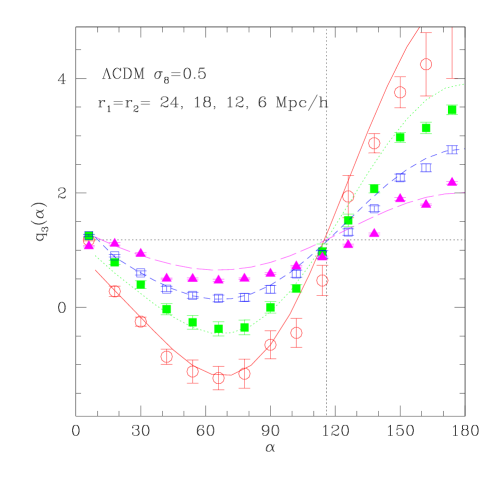
Figure 4: Plot of the value of $Q_{3}(r_{12},r_{23},\alpha)$ as a function $\alpha$ in $\Lambda CDM$ models with $\sigma_{8}=0.5$, the angle between $\vec{r}_{12}$ and $\vec{r}_{23}$, for different values of $|\vec{r}_{12}|=|\vec{r}_{23}|=24,18,12,6h^{-1}{\rm Mpc}$ (opened circles, closed squares, open squares and triangles). The corresponding lines (continuous, dotted, short-dashed and long-dashed) show the tree-level perturbation theory.

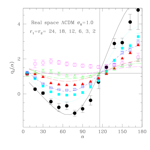
Figure 5: Same as fig.4 for the $\sigma_{8}=1$ output.

In the $\sigma_{8}=1.0$ output (fig.5) the discrepancies are significant even for $|\vec{r}_{12}|=|\vec{r}_{23}|=24h^{-1}{\rm Mpc}$. Note how deviations from tree-level tend to smooth or wash out the shape dependence for $|\vec{r}_{12}|=|\vec{r}_{23}|>12h^{-1}{\rm Mpc}$, while on smaller scales there is more shape dependence than in the tree-level, in the sense that $Q_{3}$ is smaller at smaller $\alpha$ and larger at larger $\alpha$. This tendency is also true when comparing the shape of two outputs at a given scale: i.e. the later outputs have more shape dependence than the earlier outputs at small scales ($<12h^{-1}{\rm Mpc}$), while the opposite tendency occurs for the larger scales. This effect looks similar to the ”previrialization effect” present in the 2-point function  [Scoccimarro & Frieman 1996, Lokas et al. 1996]. A similar trend was also found in the bispectrum  [Scoccimarro 1997]. The idea is that there is a change of sign in the 1-loop contribution which, for a power-law initial spectrum, is related to a critical value in the spectral index. We will study this in more detail below.

4.2 Equilateral configurations

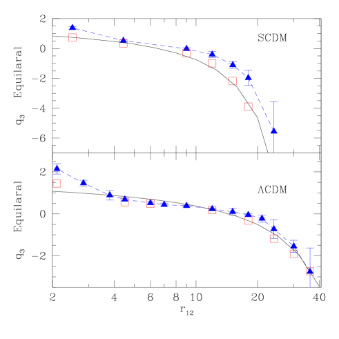
Figure 6: The normalized 3-point funciton $q_{3}$ for equilateral triangles as a funciton of the triangle side. The continuous line correspond to the PT tree-level predictions while the triangles and errors show the corresponding estimation for the mean and variance of 5 realisations in the $\sigma_{8}=1.0$ output. Opened squares show the mean of the 5 realisations in the $\sigma_{8}=0.5$ output. The top panel correspond to the $SCDM$ model while the bottom panel shows the $\Lambda CDM$ results.

Fig.6 shows $Q_{3}$ for equilateral triangles (i.e. fixed $|\vec{r}_{12}|=|\vec{r}_{23}|$ and $\alpha=60^{0}$) as a function of the triangle side ($|\vec{r}_{12}|=|\vec{r}_{23}|$), for both the $\sigma_{8}=1.0$ output (triangles) and the $\sigma_{8}=0.5$ (squares), in both the $SCDM$ (top panel) and the $\Lambda CDM$ (bottom panel) model. The dashed line just connects the points at different scales. Also shown as a continuous line is the leading order (tree-level) contribution.

For both models, the $\sigma_{8}=0.5$ output (squares) shows good agreement with the PT results. For $\sigma_{8}=1.0$ the $SCDM$ shows significant deviations from PT at all scales. On the largest scales the 2-point function goes to zero at smaller scales in the $SCDM$ model which explains why the errors are much larger around $20h^{-1}{\rm Mpc}$ in this model.

The $\Lambda CDM$ model shows larger $Q_{3}$ values than PT at $r_{12}\simeq 20h^{-1}{\rm Mpc}$ and smaller values at $r_{12}\simeq 6h^{-1}{\rm Mpc}$. This is related to the change in shape away from the leading order result noted in the subsection above (e.g. see fig.5). More in detail, at large weakly non-linear scales, $r_{12}>12h^{-1}{\rm Mpc}$ where the 2-point function is steeper (with a slope $\gamma<-2.2$) PT corrections on $Q_{3}$ are above tree-level, while for $r_{12}<12h^{-1}{\rm Mpc}$ the 2-point function is flatter (with a slope $\gamma>-2.2$) PT corrections on $Q_{3}$ are below tree-level. On smaller scales, i.e. $r_{12}<4h^{-1}{\rm Mpc}$, non-linear effects take over and $Q_{3}$ increases again above the PT results. These deviations from the leading order results are small, but significant given the sampling errors.

4.3 Loop corrections

In figure  7 we show our method to recover the tree-level and the first-loop contributions for the denominator and numerator of $Q_{3}$, i.e. for $\zeta$, and $\zeta_{H}$ respectively, as explained in subsection  3.3. All the plots in figure  7 are for a flat $\Lambda CDM$ model with $\Omega_{m}=0.2$. The plots on the left column are for isosceles triangles with equal side of $18h^{-1}{\rm Mpc}$ long whereas the ones on the right correspond to isosceles triangles with equal side of $9h^{-1}{\rm Mpc}$ long. From top to bottom, we show $\zeta$ (the 3-point function), $\zeta_{H}$ (the hierarchical combination in eq.[6]) and $Q_{3}$ (the ratio of both). In all the plots of figure  7 the solid lines correspond to the tree-level theoretical predictions from PT, the long-dashed and short-dashed lines correspond to the tree-level and 1-loop ($\sigma_{8}=1$) estimation from the 2 simulation output times, as described in eq. 13.

We can now address the question raised in the previous subsections of whether or not the relative change of sign in the deviations of $Q_{3}$ from tree-level PT (e.g. shown in fig.5 and fig.6) is related to the ”previlarization effect” on the 2-point function.

In the middle row plots we can see how for both scales ($18h^{-1}{\rm Mpc}$ and $9h^{-1}{\rm Mpc}$) the 1-loop contribution to $\zeta_{H}$ (short-dashed line) is lower than the tree-level one (long-dashed line); this can be interpreted in both cases as the well-known effect of previrialization found in the 2-point function  [Scoccimarro & Frieman 1996, Lokas et al. 1996]. But here, we have to bear in mind that $\zeta_{H}$ is a product of two 2-point correlation functions.

In the top panels one can see how the 1-loop contribution to $\zeta$ (short-dashed lines), are larger than the tree-level contribution around $\alpha\simeq 60$ deg. for $18h^{-1}{\rm Mpc}$, while they are smaller than tree-level for $9h^{-1}{\rm Mpc}$. This effect is the one mostly responsible for the relative change shown in $Q_{3}$ (smoothing/enhancing the shape with respect to the tree-level). Thus, we see that this tendency is not just given by the same critical scale index in the 2-point previrialization, as here we found a case where there is change of sign at the 3-point function level (when comparing $18h^{-1}{\rm Mpc}$ with $9h^{-1}{\rm Mpc}$ results), but not for the 2-point function. This is not surprising, as there are different PT terms contributing to each of these expressions.

In figure  8 we compare the 3-point correlation function ($\zeta$), the hierarchical 3-point correlation function ($\zeta_{H}$) and the full $Q_{3}$ parameter for the model $hSCDM$, on the left column, which has $\Omega_{m}=1$, $h=0.3$ (see table  1) to the corresponding values in the $SCDM$ model, on the right column, with $\Omega_{m}=1$, $h=0.5$ (the old standard, see table  1 ). As before the solid lines correspond to the theoretical results in PT. The short-dashed shows the $\sigma_{8}=0.5$ output. On the left panel, the short-dashed and long-dashed lines correspond to the tree-level and 1-loop reconstruction in the SCDM case. The purpose of this figure is to illustrate how the $\zeta$, $\zeta_{H}$ and $Q_{3}$ functions change with the cosmological model. The $hSCDM$ model has an approximate shape parameter for the power spectrum $\Gamma=0.25$ whereas the $SCDM$ model has a $\Gamma=0.5$. Notice that although the shape of the curves of the left and right panels in figure  8 are quite similar the actual values in the range of the plots are different.

Figure 7: Recovering the tree-level and 1-loop contributions to the numerator (top) and denominator (middle) of $Q_{3}$, and also for $Q_{3}$ itself (bottom). The cosmological model is flat $\Lambda CDM$ with $\Omega_{m}=0.2$. The left (right) column correspond to isosceles triangles with equal side being $18h^{-1}{\rm Mpc}$ ($9h^{-1}{\rm Mpc}$) long. The solid lines represent tree-level PT prediction, the long-dashed lines shows tree-level recovered for the simulations while the short-dashed corresponds to the estimated 1-loop level in the simulations (at $\sigma_{8}=1$). For clarity, only the larger error-bars in either of the two dashed lines are shown.

Figure 8: On the left column we show results for $\zeta$, $\zeta_{H}$ and $Q_{3}$ in the $hSCDM$ model with $\Omega_{m}=1$ $h=0.3$, corresponding to isosceles triangles configurations with equal side $18h^{-1}{\rm Mpc}$. The dashed line with error-bars correspond to the $\sigma_{8}=0.5$ output, the continuous line shows the leading order PT prediction. On the right column we show the same case for the model $SCDM$ ($\Omega_{m}=1$,$h=0.5$ ). Here the criteria for lines are identical to those for figure  7.

Figure  8 also illustrates how 1-loop corrections (shown as short-dashed lines) in the SCDM tend to flatten the $Q_{3}$ curve (see bottom right plot), in a similar, but more dramatic, way as we found in the $\Lambda CDM$ model in figure  7.

4.4 Other configurations

In figure  9 we show plots for $Q_{3}$ for the $\Lambda CDM$ model with $u=r_{23}/r_{12}=1$ (top row), $u=2$ (middle row) and $u=3$ (bottom row) for two values of $r_{12}$: $r_{12}=18h^{-1}{\rm Mpc}$ for the left column and $r_{12}=12h^{-1}{\rm Mpc}$ on the right one. The solid lines correspond to theoretical perturbation theory, the long-dashed lines correspond to the tree-level recovered from simulation by using our method in eq.  13, the short-dashed lines correspond to the 1-loop level ($\sigma_{8}=1$) recovered from simulations. Note the difference range of values of $Q_{3}$ in each panel. The purpose of this figure is to compare the effects at different scale lengths. On the top left plot one can see how at somewhat large scales, $\alpha>100$ deg. simulations are below the theoretical prediction. This effect is due to volume effects (or small statistical sampling); notice that $\alpha>100$ deg corresponds to $r_{13}>43h^{-1}{\rm Mpc}$ which is above one tenth of our box side, $378h^{-1}{\rm Mpc}$. This type of volume effects produce a (ratio) bias in the estimators which is not taken into account by averaging the results over different realisations [Hui & Gaztañaga 1999]. For larger $u$ this effect is even worse. This can be seen in the bottom left panel, where the error bars increase and the estimation becomes quite uncertain.

Figure 9: On the left column we show results for the $\Lambda CDM$ model with $r_{12}=18h^{-1}{\rm Mpc}$ and on the right we show results for the same model with $r_{12}=12h^{-1}{\rm Mpc}$ .The solid lines correspond to theoretical perturbation theory, the long-dashed lines correspond to the tree-level recovered from simulation by using our method in eq.  13 and the short-dashed lines correspond to the up to 1-loop level $\sigma_{8}=1$ recovered from simulations. We only show error bars in the curve in which they are larger.

At smaller scales (right panels) volume effects are smaller and there is a general agreement of tree-level PT with simulations. Higher order corrections are small.

5 Conclusions

In this paper we have studied how to obtain the 3-point correlation function from simulations and we have compared them to the predictions of perturbation theory (PT). In order to obtain the 3-point correlation function from simulations in a reasonable amount of time we have devised a method which dramatically reduces the number of operations to be carried out. The method, explained in detail in section  3.2, basically consists of assigning a list of neighbours to every node of a previously gridded box. This method, allows us to compute the $\zeta$, $\zeta_{H}$ and $Q_{3}$ for several million particles in only a few minutes.

In section  3.3 we also propose a new method to separate from simulations the tree-level and 1-loop contribution to the 2 and 3-point functions. This allows a more clear comparison to the theoretical predictions. We obtain that on sufficiently large scales, simulations results are in good agreement with leading order perturbation theory. This seems in contradiction with the results of  [Matsubara & Suto 1994, Jing & Borner 1997]; but the contradiction is only apparent. In these previous analysis they focus on the results of small scales (less than $8h^{-1}{\rm Mpc}$). Here we have shown that next to leading order (i.e. 1-loop) corrections are important on these scales and that one needs to consider larger scales (or earlier times) in order to reach the leading order (tree-level) regime. Once this is taken into account there does not seem to be a contradiction with what was found in [Matsubara & Suto 1994, Jing & Borner 1997]. On even larger scales, the 2-point correlation goes to zero and the results are dominated by sampling errors. The goodness of the agreement and the specific scales where PT is valid, depend on the shape of the initial fluctuations (i.e. the $\Gamma$ parameter in CDM models), the redshift ($\sigma_{8}$), the particular 3-point configuration under study and the level of accuracy in the comparison (i.e. the sampling errors). For the currently favoured $\Lambda CDM$ model at $\sigma_{8}=1$ there is reasonable agreement at leading order for scales larger than $20h^{-1}{\rm Mpc}$.

We also characterise next to leading order (1-loop) corrections and find that in the $\Lambda CDM$ model they seem to change sign around $12h^{-1}{\rm Mpc}$ in $Q_{3}$ (see fig.5). At $12h^{-1}{\rm Mpc}$, loop corrections seem to cancel and the tree-level PT prediction gives a better match to the simulations at this scale than at slightly larger scales (this statement would depend on the accuracy of our determination, e.g. the size of the sample, as errors increase with scale). In section §4.3 we find that this change of sign in the 1-loop term is not clearly correlated to the critical index found in the so called ”previrialization effect” [Scoccimarro & Frieman 1996, Lokas et al. 1996] for the 2-point function and also found in the bispectrum  [Scoccimarro 1997].

We have noted a crossing of the different shape predictions at $\alpha\simeq 120$ degrees in both power-law and CDM cases, even for different values of $u$. That, is when one of the interior angle of the triplet is about $120$ the value of $Q_{3}$ is $Q_{3}\simeq 1.2$, independently of the scales involved!. This seems to be a characteristic feature of the tree-level gravitational evolution, but only holds approximately after loop corrections. We do not yet have a physical interpretation for this feature, but it could be used to test gravitational instability against observational data.

Surprisely, even though PT has been known for many years now [Peebles 1980, Fry 1984], the results presented here are the first ones to show a comparison of PT with the 3-point function in N-body simulations at the appropriate scales. Most of previous comparisons of the 3-point statistics in PT to simulations were done in Fourier space [Scoccimarro & Frieman 1996, Scoccimarro 1997, Scoccimarro 2000], in angular space [Frieman & Gaztañaga 1999] or for smoothed fields [Bernardeau 1994, Baugh, Gaztañaga & Efstathiou 1995, Bernardeau et al. 2001]. The comparison presented here for the 3-point function (in configuration space) extend, for the first time, to the weakly non-linear scales were this comparison is meaningful. Not Surprisely [Bernardeau et al. 2001], we find an excellent agreement with tree-level PT theory. Moreover we characterise the range of validity of this agreement and the next order (1-loop) corrections.

References

- [Albrecht & Stebbins 1992] Albrecht, A., Stebbins, A., Phys. Rev. Lett., 68, 2121, 1992.
- [Allen et al. 1987] Allen, T. J., Grinstein, B., Wise, M.B., Phys. Lett. B,197, 66, 1987.
- [Baugh, Gaztañaga & Efstathiou 1995] Baugh, C.M., & Gaztañaga, E., Efstathiou, G., 1995, MNRAS 274, 1049
- [Bernardeau 1994] Bernardeau, F., 1994, A&A, 291, 697
- [Bernardeau et al. 2001] Bernardeau, F., Colombi, S., Gaztañaga, E., Scoccimarro R., Physics Reports, in press, 2001. Also in: http://physics.nyu.edu/scoccima/PT/PT.html
- [Buchalter & Kamionkowski 1999] Buchalter A., Kamionkowski, M., ApJ., 521, 1-16, 1999.
- [Buchalter & Kamionkowski 2000] Buchalter A., Kamionkowski, M., ApJ.,Volume 530, Iss. 1,pp. 36-52, 2000.
- [Efstathiou et al. 1985] Efstathiou, G., Davis, M., Frenk, C. S., White, S. D. M., ApJ. Supp., 57, 241, 1985.
- [Falk et al. 1993] Falk, T., Rangarajan, R., Srednicki, M., ApJ(Lett.), 403,1.
- [Frieman & Gaztañaga 1999] Frieman J.A., Gaztañaga E., ApJ, 521, L83-L86, 1999 .
- [Fry 1984] Fry, J. N., ApJ, Part I, vol. 279, April 15, 1984, p.499-510, 1984.
- [Gangui et al. 1994] Gangui, A., Lucchin, F., Matarrese, S., Mollerach, S., ApJ, 430, 447, 1994.
- [Gangui 1994] Gangui, A., Phys. Rev. D, 50, 3684, 1994.
- [Gangui & Martin 2000] Gangui, A., Martin, J., MNRAS, vol. 313, Iss. 2, 323-330, 2000.
- [Gaztañaga & Bernardeau 1998] Gaztañaga E., Bernardeau, F. A&A, Vol..331, p.829-837, 1998.
- [Gaztañaga & Frieman 1999] Gaztañaga E., Frieman, J., ApJ., Vol. 521, Iss. 2, pp. L83-L86, 1999.
- [Gaztañaga & Mahoenen 1996] Gaztañaga E., Mahoenen, P., ApJ Letters v.462, p.L1, 1996.
- [Groth & Peebles 1977] Groth, E.J.,Peebles, P.J.E., ApJ., 217, 385-405, 1977.
- [Hauser & Peebles 1973] Hauser, M.G., Peebles, P.J.E., ApJ, 185, 757, 1973.
- [Hill et al. 1989] Hill, C. T., Schramm, D. N., Fry, J.N., Comments Nucl. Part. Phys., 19, 25, 1989.
- [Hui & Gaztañaga 1999] Hui, L.& Gaztañaga, E., 1999, ApJ, 519, 622
- [Jing & Borner 1997] Jing Y.P., Börner G., Astron. Astrophys., 318, 667-672, 1997.
- [Kofman & Pogosyan 1988] Kofman, L., Pogosyan, D.Y., Phys. Rev. Lett. B, 214, 508, 1988.
- [Linde & Mukhanov 1997] Linde, A. D., Mukhanov, V., Phys. Rev. D, 56,535, 1997.
- [Lokas et al. 1996] Lokas E.L., et al.,ApJ, 467, 1-9, 1996.
- [Matsubara & Suto 1994] Matsubara, T., Suto, Y., ApJ, 420, 497, 1994 .
- [Peebles 1973] Peebles, P.J.E., ApJ, 185, 413, 1973.
- [Peebles 1980] Peebles, P.J.E., The Large scale structure of the Universe, 1980, Princeton Univ. Press.
- [Peebles & Hauser 1974] Peebles, P.J.E., Hauser, M.G., ApJ Suppl., 253, 1974.
- [Peebles 1974] Peebles, P.J.E., ApJ Suppl., 253, 1974.
- [Peebles & Groth 1975] Peebles, P.J.E., Groth, E.J., ApJ., 196, 1-11, 1975.
- [Peebles 1980] Peebles, P.J.E.,’The Large Scale Structure of the Universe’, Princeton, Princeton University Press, 1980.
- [Peebles 1999a] Peebles, P.J.E., ApJ., 510, 531, 1999.
- [Peebles 1999b] Peebles, P.J.E., ApJ., 510, 523, 1999.
- [Salopek et al. 1989] Salopek, D, Bond, J.R., Bardeen, J. M., Phys. Rev. D, 40, 1753, 1989.
- [Scoccimarro & Frieman 1996] Scoccimarro R. & Frieman, J, ApJ, 473, 620, 1996.
- [Scoccimarro 1997] Scoccimarro R., ApJ, 487, 1-17, 1997.
- [Scoccimarro 1998] Scoccimarro, R., 1998, MNRAS 299, 1097
- [Scoccimarro 2000] Scoccimarro R., ApJ, Vol. 544, Iss. 2,pp. 597-615, 2000.
- [Stuart & Ord 1994] Stuart, A., Ord, J.K.,’Kendall’s Advanced Theory of Statistics’, Vol.1 Distribution Theory, John Wiley & Sons, Edition, 1994.
- [Turok 1989] Turok, N., Phys. Rev. Lett., 63, 2625, 1989.
- [Vachaspati 1986] Vachaspati, T., Phys. Rev. Lett., 57, 1655, 1986.
- [Vilenkin 1985] Vilenkin, A., Phys. Rep., 121, 263, 1985.
- [Wang & Kamionkowski 2000] Wang, L., Kamionkowski, M., Phys.Rev.D, 61, 063504, 2000.