Harmonic analysis of cosmic microwave background data
I: ring reductions and point-source catalogue

Abstract

We present a harmonic model for the data analysis of an all-sky cosmic microwave background survey, such as Planck, where the survey is obtained through ring-scans of the sky. In this model, resampling and pixelisation of the data are avoided. The spherical transforms of the sky at each frequency, in total intensity and polarization, as well as the bright-point-source catalogue, are derived directly from the data reduced onto the rings. Formal errors and the most significant correlation coefficients for the spherical transforms of the frequency maps are preserved. A clean and transparent path from the original samplings in the time domain to the final scientific products is thus obtained. The data analysis is largely based on Fourier analysis of rings; the positional stability of the instrument’s spin axis during these scans is a requirement for the data model and is investigated here for the Planck satellite. Brighter point sources are recognised and extracted as part of the ring reductions and, on the basis of accumulated data, used to build the bright-point-source catalogue. The analysis of the rings is performed in an iterative loop, involving a range of geometric and detector response calibrations. The geometric calibrations are used to reconstruct the paths of the detectors over the sky during a scan and the phase offsets between scans of different detectors; the response calibrations eliminate short and long term variations in detector response. Point-source information may allow reconstruction of the beam profile. The reconstructed spherical transforms of the sky in each frequency channel form the input to the subsequent analysis stages. Although the methods in this paper were developed with the data processing for the Planck satellite in mind, there are many aspects which have wider implementation possibilities, including the construction of real-space pixelised maps.

1 Introduction

The traditional method used to analyse the continuum distribution of radiation on the sky is through pixelisation: the calibrated measurements are projected onto pixels of a sky map, and further analysis of the data is done by means of the pixelised responses. These methods, which are most powerfully explored in the HEALPix software [Górski 1999], have the advantage of providing a visual link to the reductions. Another already well-developed example of pixelisation is the IGLOO scheme developed by Crittenden & Turok (1998) and Crittenden (2000). A properly designed pixelisation scheme can, in addition, simplify the further analysis, allowing the use of fast spherical transform algorithms, and removing contaminated regions of the sky (Górski, 1994; Mortlock, Challinor & Hobson, 2001). A problem with any pixelisation of survey data is the loss of information due to the binning of the data. As a result of coverage variations, different pixels have different formal errors which complicates the application of fast spherical transforms. Pixels may be correlated with neighbouring pixels, which further complicates the analysis. The effective beam profile is unlikely to be circularly symmetric (as a result of intrinsic asymmetries as well as due to unconvolved sampling intervals) and requires the observations to be deconvolved. The effective two-dimensional beam profile applicable to a pixel therefore depends on the orientations of the scans which have contributed to it, information which is complicated to maintain. Thus, unless a range of ‘parallel maps’ with supplementary information is kept (the implementation of which would do away with most of the advantages of the pixelisation), a pixelisation of the data will inevitably lead to loss of information. This loss affects our ability to recover the statistical properties of the reduced data, and as such should be considered a potentially serious disadvantage.

The products of a survey mission like Planck (see for example http://astro.estec.esa.nl/planck) or MAP (http://map.gsfc.nasa.gov/m$\_$mm.htm) are a point source catalogue and a set of frequency maps, from which maps of astrophysical components are derived. Methods for the component separation have been developed amongst others by Hobson et al. (1998), Prunet et al. (2001) and Baccigalupi et al. (2000). In the latter paper an independent component analysis (ICA) algorithm is used to separate statistically independent signals from the frequency maps. In Hobson et al. (1998) component separation on small rectangular fields is investigated using a maximum entropy technique in the Fourier domain. The latter method has been further developed into a full sky implementation at the resolution required for the Planck survey [Stolyarov et al. 2002], with the frequency and component maps analysed in the form of their spherical transforms. The analysis of the cosmic microwave background (CMB; one of the components separated) depends ultimately on the reliability of the separation process. A major aim of the data analysis should be to derive the input for the component separation, the spherical multipoles of the frequency maps, in the most reliable way, preserving as much information as possible on formal errors and their correlations.

The analysis of data from an all-sky survey mission in which the survey is built up from circular scans can be carried out efficiently in three steps, as was done for the Hipparcos reductions (Lindegren, 1979; ESA, 1997): the first step reduces the raw measurements to ring data; the second step combines the ring data obtained over the mission to reconstruct the sphere; the third step analyses the sphere data. The Planck mission fits this model very well: data is obtained over 1 hour intervals during which the spin axis of the satellite remains in a nominally ‘fixed’ position. The collection of scientifically useful data starts at the end of a pointing manoeuvre and finishes with the start of the next manoeuvre, which moves the spin axis to the next scan position. During this interval, which is referred to as a time-ordered period (TOP), the satellite performs some 60 revolutions. The area of the sky covered by a detector during a TOP is referred to as a ‘ring’. The spinning of the satellite causes every detector $d$ to describe a small circle on the sky, each with its own specific opening angle $\alpha_{d}$ (the opening angle is equivalent to the co-latitude of the ring as seen from the spin-axis position). A slight wobble of the spin axis (nutation) widens the rings, but this effect is small relative to the beam width. Data in a ring are referred to the circle defined by the mean spin-axis position of the satellite during the TOP and the opening angle of the detector concerned. The nutation effect will simulate a small-amplitude periodic variation of the opening angle for the detector, which will be most noticeable for point sources close to the rings as observed by the three highest frequency channels. Over a one-year mission almost 9000 rings will be produced for each of the 48 High Frequency Instrument (HFI) and 56 Low Frequency Instrument (LFI) detectors.

In the harmonic model the three data analysis steps can be summarised as follows:

1. The analysis of the measured samplings per individual detector, collected over each TOP. The samples are referred to phases along reference circles of which the normal through the centre corresponds with the mean spin-axis position over the TOP. After cleaning these data from spikes (primarily resulting from very high energy radiation and particles), the phase-ordered data is collected in phase bins for further treatment. The short-term response variations are derived, using the accumulated differences between the mean responses in each phase bin and the individual contributions. After applying the response corrections, the mean sample values per bin are re-calculated and the data is ready for analysis. The first step in the analysis is the point-source transit identification. This is initially carried out on the phase-binned data, but in later iterations the point source catalogue constructed from the data is also used. The entire phase-binned signal is then fitted with Fourier components for the background signal and corrections to the assumed abscissae and intensities for all identified point sources. The corrected abscissae and intensities, with their formal errors, form the input to the point-source catalogue construction. The transit profiles of the brightest point sources are accumulated to provide the input for the central-beam-profile calibration.

2. Joint analysis of the Fourier components of the rings from all detectors operating at the same frequency, to produce the spherical transforms of the frequency maps. For each ring and each detector there is a unique coupling matrix, which describes how the spherical multipoles are projected on a small circle with a given opening angle $\alpha_{d}$ and a two-dimensional beam profile. The accumulated coupling matrices and ring harmonics for a given frequency are the input to a generalised least squares solution for the multipoles of that frequency map. In an iterative process, the long-term response variations are calibrated; calibration of the outer beam profile may also be done at this stage. The processing up to this point is very similar for scalar and polarised data [Challinor et al.  2002].

3. The analysis of the spherical multipoles of the frequency maps (for example, by means of the maximum entropy method) to extract the faint point sources, the Sunyaev-Zel’dovich clusters (Sunyaev & Zeldovich, 1980) and the spherical multipoles of the component maps, which are further analysed in the form of their power spectra.

Due to the way these steps are interlinked with geometric and response calibrations and the construction of the point source catalogue, they will require iterations before reduction results can be considered satisfactory.

The present paper focuses on the the first of the three steps mentioned above. Although this is seen here as the first step in the harmonic model for the data analysis, many considerations made in the reductions as described here are equally applicable in a more traditional pixelised approach. The second step is described in the accompanying paper [Challinor et al.  2002], and covers the reductions of the ring data to spherical multipoles of frequency maps in detail, a process which is more specific to the harmonic data model. The third step, described by Stolyarov et al. (2002), is the full-sky maximum entropy component separation. Additional aspects concerning the analysis of incomplete sky maps are discussed in Mortlock et al. (2002).

An important criterion for the implementation of the harmonic model is the stability of the spin-axis pointing. This stability is affected by two main contributors: residual velocities around the two axes perpendicular to the spin axis, which will create nutation; and external torques, which can create residual velocities. The amplitudes of the residual velocities at the start of a TOP are determined by the criteria for the nutation damping, and should be small enough not to create a significant effect (in comparison with the beam width) on the accumulated data. The nutation wobble of the spin axis and the effect of the external torques can be derived from an analysis of the satellite’s attitude in analytic form and through numerical integration. An analysis of this kind for the Planck satellite is presented in Appendix A, the results of which are summarised in Section 2.

In Section 3 we show how the data analysis in the harmonic model is closely linked with geometric and response calibrations. Details of the data analysis method are presented in Section 4. Section 5 describes the construction of the point-source catalogue and the calibration of the reference phases for the reduced TOPs. Section 5.2 presents the geometric calibrations: the focal plane geometry, the opening angle correction and the focal plane orientation correction. Finally Section 6 describes the way the data reduction and calibration processes are linked in iterative loops.

2 Attitude analysis for the Planck mission

The results of a full analytic and numerical analysis of the Planck satellite attitude are presented in Appendix A. Here we summarize those aspects which are of immediate importance for the data analysis. Though this analysis is applied to parameters associated with the Planck satellite, it can easily be modified to apply to different satellite configurations, as long as the outer product of the rotational velocity and angular momentum vectors is high with respect to the external torques acting on the satellite.

The Planck satellite is designed for a survey mission: over a period of a year the entire sky will be scanned twice, providing maps of the microwave sky at pass bands with central frequencies between 30 GHz and 857 GHz. The scanning will take place at pre-determined nominal pointings of the spin axis (pointing in a roughly anti-Solar direction). These nominal positions will not be exactly reproduced: a pointing noise of a few arcmin is expected. The satellite will rotate at a nominal velocity of 1 rpm, but small variations are expected here too. The interval of $\sim 1$ hour between two re-positioning manoeuvres of the spin axis is referred to as a TOP. During a TOP, the satellite’s spin axis will describe a relatively stable nutation ellipse in the satellite coordinate system (for as long as it remains unaffected by nutation damping), the maximum amplitude of which is determined by the residual velocities around the $x$- and $y$-axes, and should be less than 1.5 arcmin at the end of the nutation damping. The period of the nutation will be around 3 to 4 minutes, and will slowly change over the mission due to changes in the inertia tensor. The noise on the movement of the spin axis of the satellite relative to the nutation ellipse is at the arcsecond level. Such variations are not relevant for detectors with a 5 arcmin or more fwhm response beam. This allows one to incorporate a simple set of nutation ellipse parameters in the data analysis if necessary.

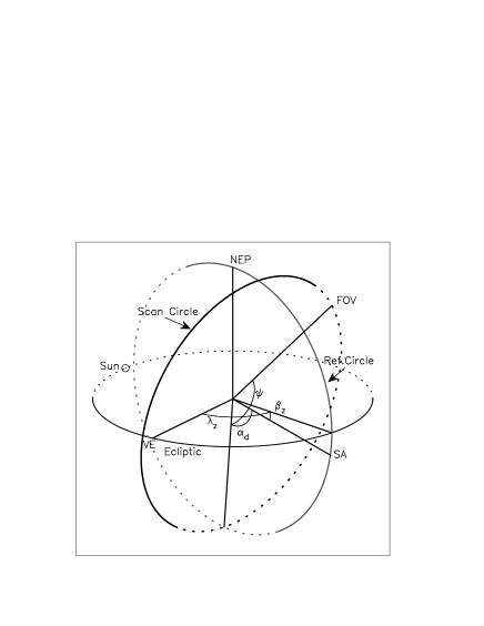
Figure 1: The orientation angles in the Planck scan. The spin axis position (SA) is defined by its ecliptic coordinates $(\lambda_{z},\beta_{z})$, measured from the vernal equinox (VE); the spin axis position and the North Ecliptic Pole (NEP) define a meridian, called the ‘reference circle’; the position of a ring is defined by its opening angle $\alpha_{d}$; the scan phase $\psi$ defines the angle between the fiducial reference point (FRP) in the field of view (FOV) and the reference circle.

The rotation of the satellite will cause every detector $d$ to describe a small circle on the sky, at an angular separation $\alpha_{d}$ (referred to as the opening angle) from the position of the spin axis (see Fig. 1). As the actual spin axis will not coincide exactly with the nominal spin axis as defined in the hardware, there will be a difference between the actual opening angle and its hardware specification value. The wobble of the spin axis slightly widens the ring, but for most detectors the beam width is such that this can be ignored. This may not be the case for the highest frequency detectors, where the spin axis wobble may add a little to the beam width as observed perpendicular to the scan direction. The way it does so will be unique to each ring set due to the variable conditions at the end of nutation damping (see Appendix A).

We can conclude that, within the model presented, the attitude of the satellite can be described in a simple manner, while the actual attitude motions do not cause any problems for the harmonic analysis of the data. The chance of significant unaccounted forces acting on the satellite, which could disturb this situation, is small.

3 The harmonic data model and system calibrations

The harmonic data model aims to provide an accurate analysis of the data and its statistical properties. It does so through a sequence of reduction steps, resulting in frequency maps in the form of spherical multipoles with their covariance matrices and a list of point source positions and intensities with associated formal errors. These maps can then be used as input for the component separation process, which can be performed in spherical multipole space [Stolyarov et al. 2002]. It should be possible to derive the spherical transforms of the frequency maps from the Fourier components of the rings, using information on pointing, focal plane geometry, focal plane orientation, the opening angle, the noise correlations of the data and the beam profile, although a number of computational problems makes this stage non-trivial [Challinor et al.  2002].

The Planck mission is designed to obtain full-sky surveys at nine different wavelengths. It explores new ranges of resolution, coverage and sensitivity at these wavelengths. For such pioneering observations, calibrations are best done by demanding internal consistency of the observed sky, which in most cases will not have changed from one observation to the next. The exceptional variable and moving sources should all be identifiable. Demanding internal consistency defines simple, differential reduction procedures, and should result in mission products with the highest possible internal precision. Absolute calibrations are carried out only in the final stages of the data processing, using a selection of sources that can be assigned and measured in a well-controlled way with ground-based or other suitable experiments. It is important during the absolute calibrations to consider the spectral response of each source and its convolution with the Planck passbands, and any background contributions which may be differently perceived by different instruments. The latter applies in particular to calibration sources close to the galactic plane.

The preference for an internal, differential calibration applies to both responses and geometric properties. For the responses it involves the following steps:

1. The short-time response variations (time scales from one minute to one hour) are calibrated as part of the ring reductions, using the phase-binned data (see Section 4.4). They show up by displaying, as a function of time, the differences between the mean samples per bin and the individual contributions to each bin. Removing any systematic effects observed in these residuals reduces all data contained in one TOP to an arbitrary mean response level for a specific detector and ring. All variations at shorter time-intervals are reduced to noise contributions, some of which may be correlated between neighbouring samples. This is taken into account in the noise correlation matrix for the model-fit solutions.

2. The long-term response variations (with time scales from one hour to one year) are calibrated as part of the sphere reductions. The reconstructed spherical transforms will, in the first instance, represent an average of all mean ring responses. By relating (in Fourier space) the response of each ring to this mean sky, response corrections per ring and detector are obtained. This is the equivalent of de-striping [Revenu et al. 2000], though in the method proposed here all data on the ring will contribute. In case the instrument high-pass filters the signal, and there is essentially no information left on the monopole, these adjustments can still be done on the remaining signal. The response-corrected rings can be used again in a reconstruction of the spherical transforms, which should result in a decrease in the fitting noise. The process can be repeated until no further significant changes to the ring responses are observed. Given the expected large number of rings involved (9000 per detector), this process is expected to converge quite rapidly. The Hipparcos reductions have demonstrated the validity of this approach in the iteration between the great circle reduction, the sphere reduction and the improvements to the astrometric parameters, which was based entirely on internal consistency of the data (see for example van Leeuwen, 1997). External information may be used to obtain a reasonable first estimate of the calibration parameters to ensure a rapid convergence of the process.

3. The last step in the response calibration adjusts each final spherical transform of a frequency map using a set of ground-based (or other) calibration sources (see above), thus transforming them from relative to absolute scales.

The result of these processes is a set of frequency maps whose precision is entirely determined by the internal calibrations, and accuracy by the quality and quantity of external calibration sources. At any stage, should improvements in external sources become available, the external calibration can be performed again. In addition, as no external information is used in the internal calibrations, the loss of information from the original data is minimal. The loss is determined primarily by the limitations in the modelling of detector response variations. If instead, for example, properties of the dipole are used in the earlier calibration steps, the extraction of independent information on the dipole from the Planck data could be compromised. The accuracy of the calibration parameters would depend on the local amplitude of the dipole signal as projected on a ring, which varies strongly with the ecliptic longitude of the spin axis.

The response or beam profile forms the link between the detector response and the detector pointing. The calibration of the central part of the beam profile is closely linked with the geometric calibrations and the construction of the bright point source catalogue. The geometric calibrations determine the pointing of each detector at any time during the observations. The relation between pointing and time can depend on the following elements:

1. The ecliptic coordinates of the mean position of the spin axis during a TOP: $(\lambda_{z},\beta_{z})$ (see Fig. 1). This position and the position of the North ecliptic pole define a great circle, referred to as the ‘reference circle’.

2. For each TOP the nutation ellipse parameters $t_{0}$, $\omega_{x,0}$, $\omega_{z}$, $f_{1}$ and $f_{2}$ as defined in equation (58) in Appendix B. The first two of these determine the $x$-amplitude and phase of the nutation ellipse, the other three determine the period and the ratio between the $x$ and $y$ amplitudes. The nutation ellipse is described in the satellite coordinates of the inertial reference system, as defined in Appendix A. When observed on the sky, the ellipse is itself rotating at the spin velocity of the satellite. The nutation period changes slowly due to variation in $f_{1}$ and $f_{2}$ resulting from depletion of consumables on-board the spacecraft.

3. The spin velocity $\omega_{z}$ and its linear dependence on time during a TOP. The latter is again a parameter which changes very slowly over the mission.

4. For each TOP, the time of the first transit of the fiducial reference point (FRP) in the focal plane through the reference circle. A first approximation can be obtained from, for example, the star mapper data and the calibration of the star mapper position with respect to the focal plane geometry. Corrections to the time of first transit are obtained during construction of the point-source catalogue.

5. The angle between the FRP and the mean spin axis position (the opening angle $\alpha_{0}$, where the index ‘0’ indicates the FRP rather than a specific detector ‘$d$’). This is a correction to the ground-based calibration value, that will change slowly with time due to inertia tensor changes.

6. The focal plane geometry, which describes, for an assumed orientation of the focal plane assembly, the coordinates of all detectors as projected on the sky, relative to the projection of the FRP in the focal plane.

7. The focal plane orientation correction, describing the difference between the actual and the assumed orientation of the focal plane as a function of time.

While items (i), (ii) and (iii) are probably best derived from the star mapper data, items (iv) to (vii) rely entirely on information contained in the science data, in particular on transits of bright point sources. Starting values for the focal plane geometry will be obtained from the instrument design specifications, but still need to be verified in flight. The calibration of these parameters relies on observed abscissae and intensities of point sources for different detectors. The geometric calibrations are crucial to the reliability of the final mission products, and inevitably require a number of iterations through the data reduction and calibration processes. As a part of these iterations the bright point-source catalogue (BPSC from here on) is produced. The BPSC provides the best possible relative positions and intensities of all brighter point sources detected by Planck, and is finally used to calibrate the overall positional reference system to the International Celestial Reference System (ICRS; Kovalevsky et al. 1997).

With the development of the BPSC, the calibration of the central beam profile can gradually be improved. In the first iteration through the data it is necessary to assume that all point sources pass through the centre of the beam. If, to a first approximation, the beam is represented as a two-dimensional Gaussian, then this assumption will do no harm: the width of the beam profile is in this case not a function of the ordinate of the transit. During subsequent iterations the ordinates of the transits can be calculated using the geometric calibrations and point-source coordinates contained in the catalogue. Ordinate information can also be incorporated in the beam profile calibrations. The construction of the catalogue ensures that in the final iteration a complete sample of point sources (up to a maximum ordinate depending on the beam profile) are taken into account in the ring analysis. This is essential for the use of such data in the sphere analysis [Challinor et al.  2002].

The iterations through the data reductions are essential due to the fact that many of the instrument calibration parameters have to be derived from the science data itself. This applies to both the response and the geometric calibrations. The precision with which these parameters can be determined is an essential part in the final data-quality verification. Poorly determined parameters will inevitably leave their mark on the final data products. The data analysis needs to identify any such parameters and their possible effect on the data as part of its preparation for the scientific exploration.

4 The ring analysis

The inputs to the ring analysis are the samples collected during a TOP for a single detector, supplemented by timing information (an absolute time for the first sample and a sampling length). It is assumed here that these intervals can be recognized from the satellite’s housekeeping data. The reference position of the spin axis during a TOP is defined as the centre of the nutation ellipse actually described by the spin axis, and is derived from the star mapper data processing. Each detector $d$ describes a small reference circle with opening angle $\alpha_{d}$ around the reference spin axis position.

The use of rings as an intermediate step in the data analysis of a full-sky survey mission was first proposed by Lindegren (1979) for the Hipparcos mission. The idea was independently explored for CMB surveys by Delabrouille, Górski & Hivon (1998), who investigated the recovery of the CMB power spectrum directly from the ring data..

4.1 Signal representation

The signal for the sky can be considered as consisting of three components: a continuous background, extended sources (which are not separated from the background) and point sources of various intensities. Translating this signal into the data observed on a given ring, a number of effects have to be taken into account:

• The satellite is rotating at a scan velocity which is not a fixed value and which may in addition change slightly during a TOP;

• The sky signal is convolved with a beam profile and sampled;

• The sky signal has a (not necessarily constant) background signal added to it, originating from the instrument itself;

• The sky signal is represented on an arbitrary and possibly slightly variable readout scale.

Some of these effects are removed in the ring reductions, others in the construction and calibration of the harmonic frequency maps [Challinor et al.  2002].

In the analysis of a TOP, two types of contributions are solved for:

1. The Fourier components, representing the structure in the underlying continuum of the microwave sky and extended sources: $C_{0}$, $C_{n}$ and $S_{n}$, with $n=1,\dots,{n_{\mathrm{m}ax}}$;

2. The intensities and abscissae for point sources (ordinates are assumed zero or obtained from the point-source catalogue): $I_{k}$ and $\psi_{k}$, with $k=1,\dots,s$, $s$ being the number of sources solved for.

In addition, the following properties of the data are resolved:

1. The detector response variations, such as changes in the background signal, $\Delta b(t-t_{\mathrm{r}})$, and drifts in the quantum efficiency, $\Delta q(t-t_{\mathrm{r}})$, where $t_{\mathrm{r}}$ is an arbitrary reference time;

2. The covariance matrix of the measurement noise. This will be the noise on bin-averaged data rather than individual samples (see Section 4.4).

The Fourier components for all TOPs corresponding to detectors in the same frequency channel are used to reconstruct the spherical multipoles of the frequency maps [Challinor et al.  2002]. This complements the “ring-torus” methods developed by Wandelt & Hansen (2001) for power spectrum estimation from the analysis of ring data from a special class of scans. The methods required for harmonic map-making also draw heavily on the harmonic-space convolution algorithms developed by Wandelt & Górski (2001) and Challinor et al. (2000). The ring analysis is iterated with the construction of the BPSC (see Section 5) by means of the geometric calibrations mentioned in Section 2. The complete inclusion of identified point sources is also ensured through the BPSC. The success of this iteration determines the final pointing noise uncertainties and their contributions to the noise on the frequency maps.

4.2 The time-to-scan-phase relation

The first requirement for the processing of the TOP data is an accurate determination of the scan velocity and its change with time over the interval covered by the TOP. The scan velocity $\omega_{z}(t)$ determines the relation between time $t$ and a relative scan phase $\psi$ for the individual sampling intervals:

$$\psi(t)=\psi(t_{\mathrm{r}})+\int^{t}_{t_{\mathrm{r}}}\omega_{z}(t){\mathrm{d}}t.$$ (1)

The attitude simulations (Appendix A) show that the scan velocity can to high accuracy be approximated by the scan velocity at reference time $t_{\mathrm{r}}$, $\omega_{z}(t_{\mathrm{r}})$ , and a constant scan-velocity drift, $\dot{\omega}_{z}$ , as

$$\omega_{z}(t)=\omega_{z}(t_{\mathrm{r}})+(t-t_{\mathrm{r}})\dot{\omega}_{z},$$ (2)

giving the following relation for $\psi(t)$:

$$\psi(t)=\psi(t_{\mathrm{r}})+(t-t_{\mathrm{r}})\omega_{z}(t_{\mathrm{r}})+\frac{1}{2}(t-t_{\mathrm{r}})^{2}\dot{\omega}_{z}.$$ (3)

A further disturbance on the time to scan phase relation comes from the wobble of the spin axis, but this is very small as is shown in Appendix B.

The scan velocity and its variation will most probably be derived from the star mapper data. However, Section 4.8 shows how information on the scan velocity is, in principle, also present in the science data. There may occasionally be a discontinuity in the relation between time and scan velocity due to semi-discrete torques caused by the satellite being hit by a micrometeorite.

Using equation (3), phases can be assigned to each sample within the TOP. Sorting the data explicitly or implicitly (through a reference index) on $\psi$ modulo $2\pi$ produces the phase-ordered data (POD) for a TOP. The use of POD has also been explored by Wandelt & Hansen (2001) in the context of power spectrum estimation. The further processing of the POD involves the following steps, which are described in detail in the sections below:

1. Spike detection is performed on the POD, where spikes will show up more clearly due to the $\sim 55$ times higher density of data points (Section 4.3);

2. Phase binning of the data: This achieves a very significant compression of the data without significant loss of information (Section 4.4);

3. Corrections for short-term detector response variations (Section 4.5);

4. Point source identification: either from the data stream itself or from the point-source catalogue, providing abscissae, ordinates and intensities (Section 4.8);

5. Signal fitting: solving for the Fourier components representing the continuum and corrections to some of the point-source parameters, and the noise spectrum (Section 4.9);

Processes (i), (ii) and (iii) are applied only once to the data, while processes (iv) and (v) are part of the iteration with the BPSC construction.

4.3 Spike detection and removal

In the POD spikes will be much more conspicuous than in the TOD, as data points are compared with others at almost identical telescope pointings. Filters have to be developed that can reliably detect spikes as outlying points. All spikes are to be removed, while their times and intensities should be collected to allow for tests of their statistical properties (distribution over time and intensity). It may also be necessary to remove the sample(s) immediately following a spike in the TOD, and to compare observed response variations for detectors with the occurrence of spikes. Confusion between spikes and transient objects should be carefully avoided. Once the POD has been searched for, and cleaned from, spikes, it is ready for further analysis.

4.4 Phase binning of the ring data

A typical TOP for an HFI detector will contain around $7\times 10^{5}$ samplings (200 Hz sampling frequency). The Fourier analysis is likely to require an $l_{\mathrm{m}ax}$ value of around 2500, giving some 5000 unknowns (see Section 4.7). The process of phase binning compresses the ring data without significantly modifying it (as would be the case when resampling), and as a result does not inflict a significant loss of information. The compression of the data, typically by a factor of 40 to 50, significantly reduces the processing time and data storage requirements. Relative to the original observations, the phase-binned data provides a much improved basis for the detection of point sources and detector response variations. The phase binning works for both point sources and the harmonic analysis of the background signal and is based on principles developed for, and used extensively in, the Hipparcos data analysis of the 1200 Hz modulated main detector signal (ESA, 1997; van Leeuwen, 1997).

The basic relation between an observation (one sampling $O_{i}$ by a single detector) and its Fourier representation is given by

$$O_{i}=C_{0}+\sum_{n=1}^{n_{\mathrm{m}ax}}\bigl{[}C_{n}\cos n\psi_{i}+S_{n}\sin n\psi_{i}\bigr{]}+N_{i},$$ (4)

where $\psi_{i}$ is the phase of the observation and $N_{i}$ represents the instrument noise. We will use this representation to describe the signal with all bright point sources removed. The ring is divided into $m$ phase bins of equal length $2\pi/m$. The phase at the centre of each bin is given by $\Psi_{j}=2\pi j/m$. Every observation is associated with a bin $j$, which turns equation (4) into

$$O_{i} = C_{0}+\sum_{n=1}^{n_{\mathrm{m}ax}}\bigl{[}C_{n}\cos n(\Psi_{j}+{\mathrm{d}}\psi_{ij})$$ (5)

$$+S_{n}\sin n(\Psi_{j}+{\mathrm{d}}\psi_{ij})\bigr{]}+N_{i},$$

where ${\mathrm{d}}\psi_{ij}=\psi_{i}-\Psi_{j}$. This can be further expanded to

$$O_{i} = C_{0}+\sum_{n=1}^{n_{\mathrm{m}ax}}\biggl{[}C_{n}(\cos n\Psi_{j}\cos n{\mathrm{d}}\psi_{ij}$$ (6)

$$-\sin n\Psi_{j}\sin n{\mathrm{d}}\psi_{ij})+S_{n}(\sin n\Psi_{j}\cos n{\mathrm{d}}\psi_{ij}$$

$$+\cos n\Psi_{j}\sin n{\mathrm{d}}\psi_{ij})\biggr{]}+N_{i}.$$

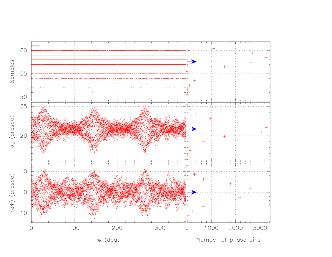
Figure 2: Results for a binning experiment at the highest Planck resolution: 5 arcmin, using 12500 bins. On the left are shown the actual values per phase bin as observed, on the right the histogram of the distribution of observed values, with an arrow indicating the expected mean value. Top graph: number of samples per bin; middle graph: phase dispersion per bin; bottom graph: mean phase offset per bin.

Phase binning provides weighted means per bin $j$ for the left- and right-hand sides of equation (6). The weights for all contributions in a bin can be taken equal. If $n_{j}$ denotes the number of samples in bin $j$, then the following relation is obtained for the mean signal in a bin:

$${\cal O}_{j} = \frac{1}{n_{j}}\sum_{i\in j}O_{i}=C_{0}+\sum_{n=1}^{n_{\mathrm{m}ax}}\biggl{[}$$

$$C_{n}\bigl{(}\Sigma_{{\mathrm{c}},j}\cos n\Psi_{j}-\Sigma_{{\mathrm{s}},j}\sin n\Psi_{j}\bigr{)}$$

$$+S_{n}\bigl{(}\Sigma_{{\mathrm{s}},j}\cos n\Psi_{j}+\Sigma_{{\mathrm{c}},j}\sin n\Psi_{j}\bigr{)}\biggr{]}+{\cal N}_{j},$$

where $\Sigma_{{\mathrm{s}},j}$ and $\Sigma_{{\mathrm{c}},j}$ are defined below. By choosing the bin size sufficiently small, the sums over the bins can be estimated. Experience with the Hipparcos data [ESA 1989] showed that a coverage of a full cycle of the highest spatial frequency by 6 bins is sufficient, and allows for the following approximations to be made:

$$\Sigma_{{\mathrm{s}},j} = \frac{1}{n_{j}}\sum_{i\in j}\sin n{\mathrm{d}}\psi_{ij}\approx\frac{n}{n_{j}}\sum_{i\in j}{\mathrm{d}}\psi_{ij}=n\langle{\mathrm{d}}\Psi_{j}\rangle,$$

$$\Sigma_{{\mathrm{c}},j} = \frac{1}{n_{j}}\sum_{i\in j}\cos n{\mathrm{d}}\psi_{ij}$$ (8)

$$\approx 1-\frac{n^{2}}{2n_{j}}\sum_{i\in j}({\mathrm{d}}\psi_{ij})^{2}=1-n^{2}\sigma^{2}_{\Psi_{j}}.$$

Depending on the amplitude of the nutation ellipse relative to the beam width, it may be necessary to fit the data contained in a phase bin as a second-order function of the offset from the reference ring position, primarily to avoid an intensity bias and noise increase due to point sources.

The phase binning thus requires the accumulation of four items per bin: the mean count ${\cal O}_{j}$, the total number of samples $n_{j}$, the average phase correction $\langle{\mathrm{d}}\Psi_{j}\rangle=\sum{\mathrm{d}}\psi_{ij}/n_{j}$ and the phase dispersion $\sigma_{\Psi_{j}}=\sqrt{\sum({\mathrm{d}}\psi_{ij})^{2}/2n_{j}}$. Values for $\langle{\mathrm{d}}\Psi\rangle$ and $\sigma_{\Psi}$ are shown in Fig. 2 for a simulation using a sampling frequency of 200 Hz, ${n_{\mathrm{m}ax}}=2050$, and 12500 bins. The offset from the nominal scan velocity was 1.243 arcsec ${\mathrm{s}}^{-1}$, and the scan velocity drift was 0.009 arcsec ${\mathrm{s}}^{-2}$. An average of 57 samples per bin is expected under these conditions. The expected value for $\langle{\mathrm{d}}\Psi\rangle$ is zero, and $\langle\sigma_{\Psi}\rangle=(\pi/m)/\sqrt{6}$ (where $m$ is the total number of bins), which equals $21\aas@@fstack{\prime\prime}6$, equivalent to 5.8 per cent of the beam dispersion, or 5 per cent of the bin width in this example.

The phase-binned data ${\cal O}_{j}$ and $\langle{\mathrm{d}}\Psi_{j}\rangle$, $\sigma_{\Psi_{j}}$ and the correlation matrix of the ${\cal N}_{j}$ enter our model of the response through equations (LABEL:equ_fou4) and (8) in a generalised least squares solution for the $\{C_{n},S_{n}\}$.

In the evaluation of equation (8) we ignored the fourth order term, which has an expected value of $(n\pi/m)^{4}/120$. With $m=6n$ for the highest $n$ value used, this amounts to a maximum correction of $6\times 10^{-4}$ to $\Sigma_{{\mathrm{c}},j}$. This figure should be compared with the expected amplitudes for the highest frequency harmonics (which will be severely depressed by the beam convolution), relative to the noise on the measurement ${\cal O}_{j}$. For the lower frequencies the contribution of the fourth order term is very much smaller still (e.g. $6\times 10^{-12}$ for $n=25$). In fact, for most of the lower frequencies the approximations of $\Sigma_{\mathrm{s}}\approx 0$ and $\Sigma_{\mathrm{c}}\approx 1$ can be used.

Thus, phase binning brings down the number of observations used for the ring analysis by a factor $\sim 57$, without any significant loss of information. The data storage requirements are as a result significantly reduced. All trigonometric coefficients in the analysis are fixed in the binned solution, and can be pre-calculated. The phase-binned data for each ring can be kept as intermediate data products, as the contents do not change in the iterative processes.

4.5 Short-term response variations

As stated before (Section 4.1), the short-term response variations can be derived from the systematic differences between the individual sample counts and the mean count of the phase bin to which the sample has been assigned. Correlated noise between neighbouring samples will transfer to similar noise between neighbouring bins. Two types of corrections can be made:

• A background variation correction $\Delta b(t-t_{\rm r})$, which can represent effects like changes in the radiation received from the instrument and the spacecraft, and which acts like a varying constant offset;

• A quantum efficiency variation correction $\Delta q(t-t_{\rm r})$, which will produce residuals scaled by the mean bin count.

For a sample $O_{i}$ in phase bin $j$ with mean count ${\cal O}_{j}$, this means

$$\Delta O_{ij}\equiv O_{i}-{\cal O}_{j}=\Delta b(t-t_{\rm r})+\Delta q(t-t_{\rm r}){\cal O}_{j}+N_{i}.$$ (9)

The functional representation for these two corrections has to be decided upon early in the mission, on the basis of the features shown in the data. A fit with a low-order spline function will in most cases take care of any real variations. At this stage it is unnecessary, and potentially even damaging, to reduce the detector responses to an absolute scale, in particular if those calibrations would include a dependence on the phase angle $\psi$, for which the reference phase has not been accurately determined yet.

The observed variations should be compared with temperature records for the spacecraft and payload and the occurrences of spikes, and correlations may be used in the removal of any observed variations. As a result of this calibration, the data collected during each TOP will be free from short-term detector variations.

4.6 Corrections for the satellite’s motion

The Planck satellite will be positioned in a Lissajous orbit around the L2 Lagrangian point of the Sun-Earth system. It will therefore describe an almost circular orbit about the Sun with a one year period and a radius of $\sim 1.01$ AU. The period for the Lissajous orbit relative to L2 is around 179 days, and will have an amplitude of around $10^{5}$ km. Thus, the orbital velocity of the satellite is dominated by its motion around the Sun and will be approximately 30.3 km s^-1. This causes fractional spectral shifts of $\Delta\lambda/\lambda\approx 10^{-4}$, which is equivalent to 9 per cent of the dipole signal in the CMB radiation. The Planck mission aims at detecting much smaller anisotropies in the CMB, and these effects are therefore a significant distortion of the signal. The effect will be opposite in the two half-year surveys, and will be most noticeable near the ecliptic plane.

The data can be corrected for this effect iteratively with the production of the frequency maps. The frequency maps can be prepared to relatively low values of $l_{\mathrm{m}ax}\approx 500$ to produce all-sky spectral index maps. The velocity vector of the satellite together with estimated maps of the spectral gradient can then provide corrections to the observed intensities for each ring:

$$\Delta I\approx\lambda\frac{\partial I}{\partial\lambda}\frac{v}{c}\cos\theta,$$ (10)

where $\theta$ is the angle between the velocity vector of the observer (which has magnitude $v$) and the observation direction, $c$ is the speed of light in vacuum, $\partial I/\partial\lambda$ is the local spectral gradient, and $\Delta I$ the local intensity correction. This effect then has to be integrated over the spectral response of the beam profile to correct the actual observed signal.

The positional effect, generally referred to as aberration, is, to first order in $v/c$, given by

$$\sin\Delta\theta=(v/c)\sin\theta,$$ (11)

where $\Delta\theta$ is the difference between the propagation direction of the radiation in a stationary reference frame and the actual moving reference frame. For the Planck observations $\Delta\theta$ has a maximum of 20 arcsec (for the part of the scan nearest to either of the ecliptic poles) and can in principle be taken into account when assigning scan phases to the individual samples. This is likely to be relevant for the HFI detectors, for which the maximum correction is comparable with the abscissa accuracies for bright point sources, and the angular scale of the highest harmonics used in the signal analysis. Ignoring the correction will result in information leakage between neighbouring frequencies in the harmonic analysis, and a significant positional noise contribution for point sources near to the ecliptic poles.

4.7 Resolution requirements

An important aspect of the realization of the harmonic data model is the value of ${n_{\mathrm{m}ax}}$ that should be applied to the data analysis. This value is largely determined by the beam width, the scan density, and the way in which point sources are dealt with in the analysis. Good estimates for ${n_{\mathrm{m}ax}}$ can be obtained by assuming a circular-symmetric Gaussian beam profile. The power spectrum of a point source convolved with a Gaussian beam is shown in Fig. 3. It is clear that in order to represent the point sources adequately as components in the harmonic analysis relatively high values of $n_{\mathrm{m}ax}$ are required. An alternative approach is to treat identifiable point sources as separate components in the ring analysis. This should be feasible if no features are expected in the background signal, which are sharp compared to the beam profile.

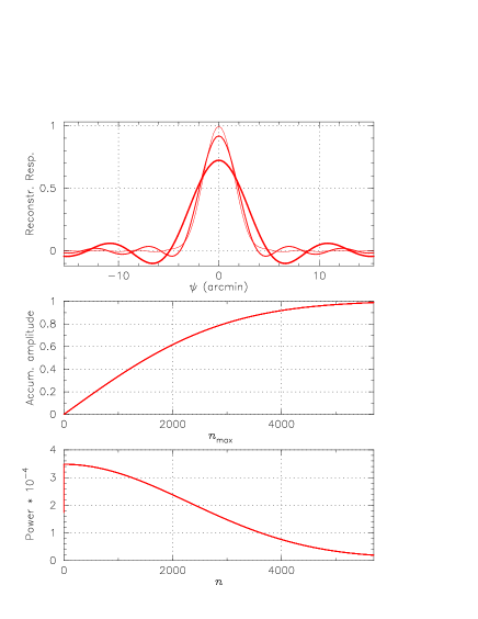
Figure 3: Bottom graph: The power spectrum of a point source (with sampled peak intensity equal to 1) given a Gaussian beam with fwhm of 5 arcmin ($\sigma_{b}=2.12$ arcmin) and a sample width of 1.8 arcmin. Middle graph: the restored peak intensity of a point source if fitted with harmonic components up to the indicated $n_{\mathrm{m}ax}$ value. Top graph: the restored point source for $n_{\mathrm{m}ax}=2500$ (thick), 4000 (intermediate) and 6000 (thin) (also distinguished by increasing peak height and decreasing side-lobe amplitudes).

A circular symmetric Gaussian beam with a dispersion $\sigma_{b}$ (in radians) will reproduce the higher harmonics in the background signal with decreased amplitudes. If the beam is represented by

$$R(\psi)=\exp[-\psi^{2}/2\sigma_{b}^{2}],$$ (12)

then the decrease in the amplitude is given by

$${a_{lm}}^{\prime}=a_{lm}\exp[-(l\sigma_{b})^{2}/2],$$ (13)

where ${a_{l}}$ is the actual and ${a_{lm}}^{\prime}$ the observed amplitude (see also Challinor et al., 2002). Provided that point sources are treated as separate objects, the suppression of higher harmonics determines the value for $n_{\mathrm{m}ax}$ in the ring solution. For $\alpha_{d}\approx 85\degr$, simulations (to be detailed in a future paper) suggest a value of $n_{\mathrm{m}ax}\approx 4400~{}{\mathrm{a}rcmin}/\sigma_{b}$, where $\sigma_{b}$ is expressed in arcmin. Thus, for $\sigma_{b}=2.12$ arcmin (fwhm of 5 arcmin) we find $n_{\mathrm{m}ax}\approx 2100$. At such high $n_{\mathrm{m}ax}$ values the matrices involved in the transformations are very large, and the covariance matrix of the spherical multipole solution will contain around $10^{13}$ elements. Fortunately, simulations, which will be detailed in a future paper, have shown that for many plausible scanning strategies, the covariance matrix of this solution will be very sparse (some analytic approximations to the covariance matrices for simple scan strategies are also derived in Challinor et al., 2001).

4.8 The point-source parameters

The main tasks of the point source processing are the following:

• To identify from either the data stream or the BPSC the point sources present in the ring data; the source of information will depend on the iteration stage of the data reduction process;

• To supplement this list with solar system objects that may have been observed;

• To produce for each point source preliminary estimates of the intensity $I_{s}$, the abscissa $\psi_{\tau}$, and if obtained from a catalogue or ephemerides (solar system objects), the ordinate $\upsilon_{\tau}$;

• To obtain as part of the reduction of the ring data the intensities $I_{s}$ of all identified sources, and abscissae $\psi_{\tau}$ for sources with a sufficiently high signal-to-noise ratio;

• To collect the abscissa data for (re-)building the BPSC;

• To collect the profiles and fitting parameters for the brightest sources as a contribution to the beam profile calibration.

This process is clearly iterative, improving at each step the quality of the BPSC, the beam profile and the reliability of the segregation of the point sources from the data.

4.8.1 Identification of point sources

The mechanism of point source identification will depend on the iteration phase of the data reductions: in the first instance point sources will mainly be identified from the data stream itself, while in subsequent iterations the identification will rely more on the BPSC. It is expected that, at least for the high-frequency detectors, the power will be dominated at high $l$ values by point sources, which should allow for the development of a reliable filter for the detection of brighter point sources. Filters for the recognition of point sources in a one-dimensional data stream were developed and successfully applied for the Hipparcos and Tycho data reductions [van Leeuwen 1997]. Simplified versions of two-dimensional filters under development for recognition of point sources on maps (see for example Cayon et al., 2000, Sanz et al., 2001) could also be considered. The detection of point sources from the data is significantly enhanced by the phase binning of the data, increasing the signal-to-noise ratio by almost a factor 7 for the parameters used in Section 4.4.

On the first pass through the data all point sources are assumed to transit through the centre of the beam. This is not problematic if the beam is approximately circularly symmetric and Gaussian. The deviation of the actual beam profile from this assumption will cause a slight error in the first reconstruction of the beam. This error can be reduced once ordinate information on point source transits becomes available too.

All detected point sources will be used to build the first and subsequent versions of the BPSC: the evolving catalogue used in iterations to predict and consistently identify point sources. In these iterations information on the ordinate of the source at the time of the transit should also be incorporated. The consistent inclusion of point sources in the ring analysis is an essential requirement for the further analysis of the underlying continuum. The BPSC also plays a crucial role in the geometric calibrations of the instrument.

4.8.2 The measured and binned point-source signal

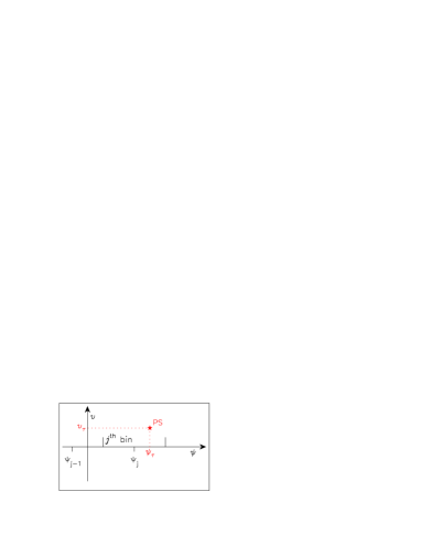
Figure 4: The point-source position (PS) relative to the phase binning and the mean scan circle.

The sampled responses $O_{i}$ for a point source of intensity $I_{s}$, passing through the beam of a detector, is a function of the scan phase $\psi_{i}$ (at the midpoint of the sampling interval) for sample $i$ and the abscissa $\psi_{\tau}$ and ordinate $\upsilon_{\tau}$ of the point source (see Fig. 4):

$$O_{i}=I_{s}\int^{\psi_{i}+\Delta\psi}_{\psi_{i}-\Delta\psi}R(\psi_{\tau}-\psi,\upsilon_{\tau}){\mathrm{d}}\psi,$$ (14)

where the integral represents the sampling interval, and $R(\psi_{\tau}-\psi,\upsilon_{\tau})$ is the normalized beam profile for a detector as a function of the offset from the centre of the beam ($\psi_{\tau}-\psi$ along the scan direction and $\upsilon_{\tau}$ perpendicular to the scan direction).

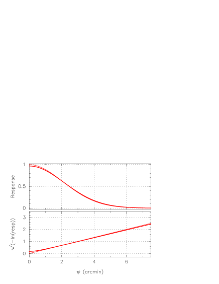
Figure 5: The beam response $R(\psi,0)$ (thin line) and the convolved beam response $S(\psi,0)$ (thick line) profiles for a Gaussian beam with fwhm$=5$ arcmin. The increase in beam width as a result of the samplingis of the order of 20 arcsec. Top graph: in linear response scale; bottom graph: in logarithmic response scale.

The effective beam profile $S(\psi,\upsilon)$ is defined as the actual beam profile $R(\psi,\upsilon)$ convolved with the sampling interval, as illustrated in Fig. 5 [see also equation (8)]

$$S(\psi,\upsilon)=\int^{\psi+\Delta\psi}_{\psi-\Delta\psi}R(\psi^{\prime},\upsilon){\mathrm{d}}\psi^{\prime},$$ (15)

where the relevant coefficients are defined in Section 4.4. When phase binning is applied to the point source contributions, the response in phase bin $j$ is given by

$${\cal O}_{j} = I_{s}\bigl{[}S(\psi_{\tau}-\Psi_{j},\upsilon_{\tau})-\langle{\mathrm{d}}\Psi_{j}\rangle S^{\prime}(\psi_{\tau}-\Psi_{j},\upsilon_{\tau})$$ (16)

$$+\sigma_{\Psi_{j}}^{2}S^{\prime\prime}(\psi_{\tau}-\Psi_{j},\upsilon_{\tau})\bigr{]}+{\cal B}_{j}+{\cal N}_{j},$$

where ${\cal B}_{j}$ represents the background signal. In the same way as was found for the harmonic multipoles, the main contribution comes from the second derivative, which produces an effective broadening of the beam. However, if we use 12 500 bins for a beam with fwhm=5 arcmin ($\sigma_{b}=2.12~{}{\mathrm{a}rcmin}$), the additional dispersion is $\sigma_{\Psi_{j}}\approx 21\aas@@fstack{\prime\prime}6$ and the effective fwhm of the beam is increased as a result of the phase binning by no more than one per cent.

4.8.3 Fitting parameters for the point-source signal

Two parameters require determination in the signal fit: the transit phase $\psi_{\tau}$ and intensity $I_{s}$ of the point source. For both, preliminary estimates are required which are then adjusted in the solution.

Equation 16 can be linearized in the intensity correction $\delta I_{s}$ and the transit correction $\delta\psi_{\tau}$ so that

$${\cal O}_{j} = \delta I_{s}S(\psi_{\tau}-\Psi_{j},\upsilon_{\tau})+\delta\psi_{\tau}I_{s}S^{\prime}(\psi_{\tau}-\Psi_{j},\upsilon_{\tau})$$ (17)

$$+I_{s}S(\psi_{\tau}-\Psi_{j},\upsilon_{\tau})+{\cal B}_{j}+{\cal N}_{j}.$$

This equation enters in the generalised least squares solution for the ring data (see Section 4.9). The intensity correction term in Eq. 17 is scaled by the response function. As a result of this, the noise on the lower intensities (the wings of the response function) will tend to affect the determination of $\delta I_{s}$ more than the better determined higher intensities (core of the response function). This is in particular the case when the noise on the signal depends on its intensity. Therefore, only a few of the central phase bins should be used for solving for the transit parameters of a given source. It may be necessary to iterate the ring solution to properly separate the point source and continuum contributions.

Assuming we use the central 5 phase bins for determining the fitting parameters for each point source, estimates can be obtained for the expected precisions. For the intensity error a value of 0.8 times the noise level on the binned samples is expected, equivalent to 0.12 times the noise level on individual samples. For the abscissa error we estimate a value of 1.7 arcmin divided by the signal-to-noise ratio of the point source in the phase-binned data.

4.8.4 Transient sources

Any object moving by a significant fraction of the beam width over an interval of one hour will have to be treated as a transient source. For the highest frequency channels of Planck this translates into a movement of approximately 2 arcmin per hour and above. The fastest objects in the Earth’s neighbourhood will be traveling at $\sim 10^{5}$ km hr^-1. The limit of 2 arcmin then translates into a horizon of around 1.2 AU, which will include a small fraction of asteroids and the occasional comet.

For sources that are not variable on a time-scale of less than one hour (which may not be true due to rotation of the objects), systematic differences between the actual measurements (before phase binning) and the reference profile can be expressed as corrections to the effective scan velocity $\omega_{z}(t_{\mathrm{r}})$ :

$$\Delta O_{i} = O_{i}-B_{i}-I_{s}S(\psi_{\tau}-\psi_{i},\upsilon)$$ (18)

$$\approx I_{s}\frac{\partial S}{\partial\psi}\Delta(\psi_{i}-\psi_{\tau})+N_{i}$$

$$= (t-t_{\mathrm{r}})I_{s}\frac{\partial S}{\partial\psi}{\mathrm{d}}\omega_{z}+N_{i},$$

which shows that most of the information on $\omega_{z}(t_{\mathrm{r}})$ is contained in those sections of the signal which have the steepest gradient as a function of $\psi$. The same kind of information can in principle also be used to determine the scan velocity from the science data using bright-point-source measurements, although it would be by far preferred to derive this information from the star mapper data.

4.8.5 Beam profile calibration

The beam profile calibration uses the accumulated transit data of bright point sources (which may include transits of solar system objects). During the first processing of the data no reliable ordinate information is available (catalogue positions are still poor or non-existent, and opening angles still need to be calibrated), and every source is assumed to go through the centre of the beam. During later stages of the data reductions, when the point-source catalogue and the geometric calibrations are improving, the ordinate information can be incorporated too.

The principle of the beam profile calibration follows techniques used in the Hipparcos data reductions for the single slit response functions of the star mapper slits (ESA, 1997; van Leeuwen, 1997). The response function is sampled at a frequency 4 to 8 times higher than the sampling frequency of the data. Using the abscissae and intensities of identified point sources, the observed residual samplings ${\cal O}_{j}-{\cal B}_{j}$ (original signal ${\cal O}_{j}$ minus the background ${\cal B}_{j}$ as estimated from the current harmonic fit to the continuum) in phase bins close to the point source transit phases $\{\psi_{\tau}\}$ are binned according to their separation from the transit phase $\{\psi_{\tau}\}$. Also accumulated in bins are the derived transit peak intensities $I_{s}$. Thus, we find for the beam-profile bin $k$ the mean normalised response

$${\cal S}(k)=\frac{\sum\bigl{[}{\cal O}_{j}(k)-{\cal B}_{j}(k)\bigr{]}}{\sum I_{s}(k)},$$ (19)

where the sums are over the point sources and phase bins contributing to the beam-profile bin $k$. Noise correlations between neighbouring bins in the phase-sampled data will also affect the accumulation of equation (19), in that pairs of bins in the accumulation can contain partially correlated noise, which needs to be taken into account when fitting a response curve. The values ${\cal S}(k)$ can be fitted with a cubic spline to provide a smooth beam profile with a continuous derivative, which then provides an estimate for the sampled beam profile $S(\psi,0)$. When, after the construction of the first point-source catalogue, ordinates become available for the point-source transits, the beam profile can be resolved in two dimensions. The reconstructed beam profile obtained this way is the sampled, effective profile, and not the actual profile, which would apply to a stationary detector.

Transits of planets such as Jupiter may also be useful for the beam profile calibration, though could be problematic: the detector response to very high intensities will not be linear, and the spectral gradient for the planets is likely to be quite different from that of the average microwave point source. The beam profiles will vary with frequency (see for example Challinor et al., 2001), making it still more complicated to incorporate the profiles measured from the planets.

4.9 The ring solution

After binning the data, calibrating and removing short-term detector responses, and identifying the point sources, the TOP is ready for reduction. This part of the reductions consists of a generalised least squares solution for the ring harmonics in the underlying continuum (equations (6)–(8)) and simultaneous solutions for the abscissa and intensity corrections for all identified point sources (equation (17)). The observation vector $\mn@boldsymbol{z}$ has as its components the mean response in each phase bin. The observations are related to the vector $\mn@boldsymbol{x}$ containing the amplitudes of the circle harmonics, $\{C_{n},S_{n}\}$, and the corrections to the point source parameters, $\delta I_{s}$ and $\delta\psi_{\tau}$, and the noise vector $\mn@boldsymbol{\nu}$, whose components are the noise in each phase bin, ${\mathcal{N}}_{j}$, via the linear equation

$${\mn@boldsymbol{z}}={\textbf{{A}}}{\mn@boldsymbol{x}}+{\mn@boldsymbol{\nu}}.$$ (20)

The matrix A depends on the locations of the phase bins, $\Psi_{j}$, the phase corrections and dispersions, $\langle{\mathrm{d}}\Psi_{j}\rangle$ and $\sigma_{\Psi_{j}}$, the current estimate of the point source intensities and positions, $I_{s}$ and $\psi_{\tau}$ (and ordinate information as this becomes available), and the current estimate of the beam profile, $S(\psi,v)$. Equation (20) is the matrix form of equations (LABEL:equ_fou4) and (17). The minimum-variance estimate of $\mn@boldsymbol{x}$ is

$$\hat{{\mn@boldsymbol{x}}}=({\textbf{{A}}}^{T}{\textbf{{N}}}^{-1}{\textbf{{A}}})^{-1}{\textbf{{A}}}^{T}{\textbf{{N}}}^{-1}{\mn@boldsymbol{z}},$$ (21)

with errors

$$\langle(\hat{{\mn@boldsymbol{x}}}-{\mn@boldsymbol{x}})(\hat{{\mn@boldsymbol{x}}}-{\mn@boldsymbol{x}})^{T}\rangle=({\textbf{{A}}}^{T}{\textbf{{N}}}^{-1}{\textbf{{A}}})^{-1},$$ (22)

where ${\textbf{{N}}}\equiv\langle\mn@boldsymbol{\nu}\mn@boldsymbol{\nu}^{T}\rangle$ is the (phase-binned) noise covariance matrix.

Assuming the instrument noise is a stationary, random process with correlation function $C(t)$ in the time domain, we can obtain the noise contribution to the mean response in a given phase bin by integrating over the time periods corresponding to those observations falling in that bin. The covariance matrix $[{\textbf{{N}}}]_{jj^{\prime}}\equiv\langle{\mathcal{N}}_{j}{\mathcal{N}}_{j^{\prime}}\rangle$ then takes the form of a convolution:

$$[{\textbf{{N}}}]_{jj^{\prime}}=\left(\frac{m}{N_{\mathrm{s}}}\right)^{2}\int_{x_{-}}^{x_{+}}\Lambda(x)C\{T_{\mathrm{s}}[x+(j-j^{\prime})/m]\}\,{\mathrm{d}}x,$$ (23)

where $N_{\mathrm{s}}$ is the number of times the ring is scanned in one TOP, $T_{\mathrm{s}}$ is the average spin period in that TOP, $m$ is the number of phase bins, and the integration limits $x_{\pm}\equiv-(N_{\mathrm{s}}-1)\pm 1/m$. The function $\Lambda(x)$ is given by

$$\Lambda(x) = \sum_{n=-(N_{\mathrm{s}}-1)}^{N_{\mathrm{s}}-1}\Bigl{[}\Theta(1/m-|x-n|)$$ (24)

$$\qquad\times(1/m-|x-n|)(N_{s}-|n|)\Bigr{]},$$

where $\Theta(x)$ is the Heaviside unit step function, and arises from the effects of phase binning and repeatedly scanning the ring. For white noise the ${\mathcal{N}}_{j}$ are uncorrelated, but in the presence of a significant low frequency component correlations will arise. Typically, instruments are designed with the goal of restricting coloured noise to frequencies below the spin frequency, in which case the correlation length of the noise exceeds the spin period. (For Planck HFI, the nominal knee frequency at which the character of the noise changes from $1/f$ to white is less than $0.06\,\mathrm{rad}~{}\mathrm{s}^{-1}$, while the spin frequency is $0.10\,\mathrm{rad}~{}\mathrm{s}^{-1}$.) As the correlation length becomes large compared to the spin period, the noise covariance matrix approaches $[{\textbf{{N}}}]_{jj^{\prime}}=\chi^{2}_{\mathrm{c}}+\chi^{2}_{\mathrm{u}}\delta_{jj^{\prime}}$, corresponding to a fully correlated offset in every bin with r.m.s. $\chi_{\mathrm{c}}$, and uncorrelated noise with r.m.s. $\chi_{\mathrm{u}}$. In practice, the noise power spectrum will have to be estimated from the data directly rather than relying on simple parameterised forms like that give above. If the correlation length exceeds $N_{\mathrm{s}}T_{\mathrm{s}}$ the offsets on different rings will generally also be correlated, so an optimal analysis would require reducing several rings simultaneously.

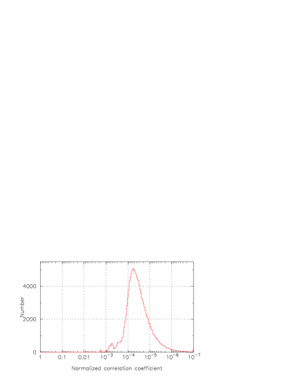
Figure 6: A histogram of the normalised, absolute values of the off-diagonal elements in the square root of the covariance matrix for a typical bin-sampled ring solution, using $l_{\mathrm{m}ax}=512$. The matrix can effectively be regarded as diagonal.

Under the assumption of Gaussianity, the relevant components of the covariance matrix $\langle(\hat{{\mn@boldsymbol{x}}}-{\mn@boldsymbol{x}})(\hat{{\mn@boldsymbol{x}}}-{\mn@boldsymbol{x}})^{T}\rangle$ determine the errors on the ring harmonics (marginalised over the point source corrections). We have conducted several simulations to investigate the effects of variations in the spin velocity, and the presence of point sources, on the covariance matrix for the errors on the ring harmonics. To isolate the effects of spin velocity and point sources we have only considered white instrument noise. For our simulations we adopted a maximum value of $n$ equal to $512$. The covariance matrix for the errors on the ring harmonics is found to be very close to diagonal if only relatively faint point sources are present. In the presence of a very bright point source (like Jupiter), which will create a very low-weight gap in the ring data, there is a minor effect on the diagonal structure of the covariance matrix, the effects being largest in low frequency detectors. The normalised off-diagonal elements in the (Cholesky) square root of a typical covariance matrix are accumulated in a histogram in Fig. 6. The results show that the correlations between the different ring harmonics are at a level of 0.2 per cent or less. These levels decrease still further with increased resolution. The inclusion of a bright point source would affect the distribution, but correlations would still be below the 1 per cent level. If we further include stationary instrument noise, we can expect the errors on the ring harmonics to still be uncorrelated between Fourier modes for large $N_{\mathrm{s}}$. If coloured noise is confined to frequencies well below the spin frequency, correlations between rings will only affect the $n=0$ modes [Challinor et al.  2002].

5 The bright-point-source catalogue

The bright-point-source catalogue (BPSC) is both a major product of the Planck mission, and an important calibration tool. The catalogue is constructed iteratively from the abscissae and intensities of the point sources obtained in the current ring reductions. Corrections to the BPSC will ultimately provide positions, intensities (at different frequencies), and variability information for all detected sources. As was explained in Section 3, the spin axis position (including nutation movements) and spin rate are most likely derived from the star mapper data, all other geometric calibrations depend at least to some extent on the science data.

5.1 The positional sphere reconstruction

The construction of the BPSC follows a simplified version of the Hipparcos sphere reconstruction process [ESA 1997]. This process requires a set of a priori positions for the point sources, to which corrections are determined. These positions are also required in order to identify consistently point-source transits on different rings with objects on the sky. Initial positions at a precision of twice the beam size (10 arcmin for Planck) will be sufficient for this purpose. Using the ground-based specifications of the focal plane geometry and inertia tensor, first estimates are obtained for the opening angle and focal plane rotation corrections, and the focal plane geometry. These estimates can be further refined through the use of planetary transits. From this information we obtain preliminary details of the alignment of the different detectors during a scan: phase offsets and effective opening angles. The transits recorded in scans for the different detectors can now be transferred to a common sky, where each transit is represented by an error ellipse, strongly elongated in a direction perpendicular to the scan direction. A simple algorithm is then required to cross identify the different transits, and to produce from the accumulated information the necessary initial positions.

Once a catalogue of initial positions has been obtained, and transits have been identified with sources in the catalogue, corrections to the assumed positions and to the reference phases of the rings can be determined. Given the ecliptic coordinates $(\lambda_{z},\beta_{z})$ of the spin axis, and a position for a point source $i$ at $(\lambda_{i},\beta_{i})$, the expected abscissa and ordinate of the point source with respect to the ring can be derived. The coordinates $(\psi_{i},\zeta_{i})$ in the system with the spin axis at the pole (where $\psi_{i}$ is measured from the reference circle as defined in Fig. 1, and $\zeta_{i}$ is the latitude of the source relative to the great circle associated with the spin-axis position) are obtained from

$$\left[\matrix{\cos\psi_{i}\cos\zeta_{i}\cr\sin\psi_{i}\cos\zeta_{i}\cr\sin\zeta_{i}}\right]={\textbf{{R}}}_{2}\bigl{(}\beta_{z}-\frac{\pi}{2}\bigr{)}{\textbf{{R}}}_{3}(-\lambda_{z})\left[\matrix{\cos\lambda_{i}\cos\beta_{i}\cr\sin\lambda_{i}\cos\beta_{i}\cr\sin\beta_{i}}\right],$$ (25)

where ${\textbf{{R}}}_{i}(\phi)$ is the matrix representing a right-handed rotation around axis $i$ through angle $\phi$. Equation (25) can be used to derive the relation between corrections to the source position $(\lambda_{i},\beta_{i})$ and the resulting changes to the scan phase $\psi$ (obtained from the transit abscissae) and ordinate $\upsilon$ (reflected in the transit intensities). We define $\zeta=\frac{\pi}{2}-\alpha+\upsilon$, where $\upsilon$ is the ordinate relative to the actual ring, and $\alpha$ the opening angle. The relations between the offset values for $(\Delta\psi_{i},\Delta\upsilon_{i})$ and $(\Delta\lambda_{i},\Delta\beta_{i})$ are then found to be

$$\Delta\psi_{i}\cos^{2}\zeta_{i} = f_{1}\Delta\lambda_{i}\cos\beta_{i}+f_{2}\Delta\beta_{i},$$

$$\Delta\upsilon_{i}\cos\zeta_{i} = -f_{2}\Delta\lambda_{i}\cos\beta_{i}+f_{1}\Delta\beta_{i},$$ (26)

where $f_{1}$ and $f_{2}$ are defined as

$$f_{1} = \sin\beta_{z}\cos\beta_{i}-\cos\beta_{z}\sin\beta_{i}\cos(\lambda_{i}-\lambda_{z}),$$

$$f_{2} = \cos\beta_{z}\sin(\lambda_{i}-\lambda_{z}).$$ (27)

For a scanning strategy where the spin axis remains in or close to the ecliptic plane (and $\lambda_{i}-\lambda_{z}\approx\pm\pi/2$), $f_{1}\approx 0$ and $|f_{2}|\approx 1$ for most sources, the exception being sources situated close to either of the ecliptic poles. The result is that very little information on the ecliptic longitudes can be extracted from the measured abscissae, except for images at high ecliptic latitudes. Some information on the longitudes can, however, be extracted using the measured intensities, which depend on $\upsilon$ through the beam profile. This method will inevitably fail when the source is variable.

The positional sphere solution consists of a least squares fit of the differences between the observed and predicted abscissae, $\Delta\psi_{i,j}$ (for point source $i$ on ring $j$) to corrections $(\Delta\lambda_{i},\Delta\beta_{i})$ for each point source. In addition, there is a correction $\Delta\psi_{j}$ to the assumed reference phase for each ring. In the solution a boundary condition needs to be included which states that the average correction $\sum\Delta\psi_{j}=0$, else a singularity may occur. When using different detectors, the phase offsets between the detectors have to remain effectively fixed: the only changes can come from rotation variations of the field of view, and focal length variations of the telescope, and both effects are unlikely to be significant.

To estimate the number of observations and parameters, we assume 10 000 point sources on the sky bright enough to be detected on single rings (Barreiro, private communication), and 10 000 rings per detector over the Planck mission. With the beam’s fwhm$=5$ arcmin, the average number of point sources detected per ring is 6 passing within $\pm\sigma_{b}$, and 6 more passing within $\pm 2\sigma_{b}$ from the mean position of the ring. The total number of transits recorded is then $\sim 10^{5}$ per detector, giving $\sim 10$ observations per source per detector. The total number of parameters to be estimated is $\sim 3\times 10^{4}$, and this does not increase when information from more detectors is used (except when some point sources are not visible for all detectors used). Increasing the number of detectors increases the number of observations and will increase the rigidity of the solution.

The relative positions of point sources obtained this way are rigid, but absolute positions are only determined up to an overall rotation, and so require linking to the International Celestial Reference Frame [Kovalevsky et al. 1997]. This can be accomplished through cross identification with radio and optical counterparts, thus determining a global rotation to be applied to the entire catalogue. This may not be important for the statistical properties of the CMB component in the background, but is relevant for relating sources and the dust map to other observations.

5.2 Geometrical calibrations

In Section 3 we mentioned four geometric calibrations which rely on the point-source data collected by the satellite:

1. The reference phase of the FRP, to be obtained for each circle;

2. The opening angle for the FRP, to be obtained as a slowly changing function of time;

3. The focal plane orientation, to be obtained as a slowly changing function of time.

4. The focal plane geometry, to be obtained as a fixed set of parameters.

The first three points concern the first order geometric orientation of the field of view: its shifts perpendicular to, and along, the scan direction, and its rotation. These result in systematic shifts in the abscissae and blurred intensity distributions for point sources, both as functions of the field of view position of the detector. The systematic shifts can be solved for as instrument parameters in the positional sphere reconstruction. This also applies to the calibration of the along-scan position of each detector in the focal plane geometry.

The opening angle for each detector can only be derived from the brightness distributions of the point sources observed with it. A maximum likelihood solution, optimizing the intensity distributions of the brightest, non-variable point sources should provide these calibration values. This can, however, only be applied to sources for which the positions on the sky are well determined in both coordinates through the positional sphere reconstruction. For the Planck mission this condition limits its application to point sources near to the ecliptic poles.

Additional information can be obtained from transits of planets and minor planets, for which the absolute coordinates at any time during the mission are known to a much higher accuracy than required for the Planck calibrations, and which have the advantage of being visible to most or all detectors. To use these transits for opening angle calibrations requires, however, accurate knowledge of the beam profile perpendicular to the scan direction as well as accurate predictions of their expected intensities, both of which may be difficult to obtain.

6 Iterations with calibrations and the ring analysis

Iterations between the point-source catalogue and the ring reductions are necessary to obtain a properly calibrated geometric reference system for the observations. Without these calibrations in place interpretation of the data in the form of (partial) maps will be of limited value, especially towards the higher frequencies in the power spectrum.

Iteration with the BPSC is also required to assign ordinates to point-source transits, which is essential in calibrating the two-dimensional beam profile. Using the BPSC for the identification of point sources in the final ring reductions ensures that the background signals for all all rings contain compatible information. Inconsistent point-source subtraction would lead to harmonic signals in the ring analysis that can not be combined in the harmonic map-making.

An iteration with the harmonic map-making [Challinor et al.  2002] for the half-year data is required to remove the spectral shift in the data which results from the velocity vector of the satellite (see Section 4.6). While the CMB dipole affects only the CMB component in the frequency maps, the satellite’s velocity vector affects all component on every frequency map in both aberration and Doppler shift.

Most of these iterations require complete reprocessing of the ring data and are, as such, very time consuming. Without them, however, the scientific interpretation of the data will be subject to considerable uncertainty.

7 Conclusions

The harmonic data model, of which the first part was presented in the current paper, provides a high level of information preservation in the data reductions. It defines calibration requirements and methods and provides a clear path from observed quantities to the scientific products. The latter is important, as the interpretation of the science products requires reliable knowledge of their statistical characteristics, which are well defined in the harmonic model.

Although the methods presented in the current paper were developed as part of the harmonic data model, most would also be useful when using the more traditional pixelisation methods. This applies, for example, to the iterative cycle of the ring reductions, BPSC construction and the geometric calibrations. Phase binning of the data can also be used with pixel-based methods, as it provides a means for short-term response calibrations, point source recognition and data compression.

Further work is in progress in areas of point-source recognition from the ring data, and the cross-identification of point sources as detected on different rings.

The part of the Planck data processing presented in this paper will be very demanding. An estimated half a million rings will be produced by the HFI per year of observations. The calibration requirements will make it necessary to process each ring at least three times to get all geometric and beam profile calibrations implemented. The processing of such large quantities of data requires careful planning.

Appendix A Planck attitude dynamics

The dynamics of the Planck satellite are largely determined by the following characteristics:

• The total mass and its variation over the mission;

• The inertia tensor and its variation over the mission;

• The position of the centre of gravity (CoG);

• The actual scan velocity, which will be very close to a fixed nominal value;

• The size, position and optical characteristics of the solar panel.

A.1 Input parameters

Early models by Matra Marconi (Dynamics and Pointing, 260/CDA/NT/83.95) have provided an initial set of values for the satellite characteristics, which we can use to derive a model for the satellite attitude. Although changes in these parameters can be expected for the final realisation of the Planck satellite, the general character of the results presented here will not be much affected.

We use the following values:

• The total mass is 772 kg;

• The inertia tensor (defined in the SRS coordinate system, see the next section) is given by

  $${\textbf{{I}}}=\left[\matrix{699&4.0&4.5\cr 4.0&766&4.2\cr 4.5&4.2&970}\right]\ {\mathrm{k}g~{}m^{2}},$$

  where the actual values used are only of relevance in as far as that they reproduce the approximate characteristics of the tensor;

• The position of the CoG, in the same reference system as defined above, is given by

  $$\left[\matrix{x_{0}\cr y_{0}\cr z_{0}}\right]=\left[\matrix{0.0319\cr-0.0315\cr\-0.7282}\right]\ \ {\mathrm{m}};$$

• The diameter of the solar panel is 4.5 m, with a secular reflection coefficient $C_{\mathrm{s}}=0.17$, and a diffuse reflection coefficient $C_{\mathrm{d}}=0.10$;

• The solar radiation pressure is $4.5\times 10^{-6}$Nm^-2.

The solar panel shields the rest of the satellite from solar radiation. Its position, size and optical characteristics therefore determine the solar radiation force experienced by the satellite. The position of the CoG then determines how much of this force is experienced as a torque (see for example Spence, 1978).

A.2 The inertia tensor and coordinate alignments

The inertia tensor given above is not diagonal, i.e. the principal axes of the satellite do not align with the principal axes of the inertia tensor. We define two reference systems; the Satellite Reference System (SRS), aligned with the principle axes of the satellite, and the Inertia Reference System (IRS), aligned with the principle $z$-axis of the inertia tensor. The origin of both systems is the CoG.

The SRS is defined as follows. The $z$-axis is normal to the solar panel, goes through the CoG and is pointing away from the Sun. The $x$-axis lies in the plane through the $z$-axis and the vector from the CoG to the FRP as projected onto the sky, and is orthogonal to the $z$-axis. The $y$-axis completes the right-handed triad.

The IRS is defined such that the off-diagonal elements $I_{xz}$ and $I_{yz}$ of the inertia tensor are zero. This is obtained by two small rotations $\alpha_{1,2}$. A third rotation ($\alpha_{3}$) is added to make $z^{\prime}$, $x^{\prime}$ and the direction of the FRP on the sky coplanar. The three rotations are clockwise around the $x$, $y$ and $z$ axes respectively, and define a rotation matrix

$${\textbf{{R}}}\approx\left[\matrix{1&-\alpha_{3}&\alpha_{2}\cr\alpha_{3}&1&-\alpha_{1}\cr-\alpha_{2}&\alpha_{1}&1}\right].$$ (28)

The inertia tensor ${\textbf{{I}}}^{\prime}$ in the IRS is related to the inertia tensor I in the SRS through

$${\textbf{{I}}}^{\prime}={\textbf{{R}}}{\textbf{{I}}}{\textbf{{R}}}^{T}.$$ (29)

The physical meaning of the angles $\alpha_{1,2,3}$ is simple: $\alpha_{1}$ is the rotation of the focal plane relative to the ring; $\alpha_{2}$ is the difference between the nominal and actual opening angle for the centre of the focal plane; $\alpha_{3}$ is an overall phase shift.

Due to the depletion of consumables, the values in the inertia tensor cannot be assumed constant. The angles $\alpha_{1,2,3}$ will change over the mission as a result of this, $\alpha_{1}$ and $\alpha_{2}$ will require calibration during the mission, while $\alpha_{3}$ corrections are absorbed in the zero-phase corrections that have to be applied to each circle.

A.3 The attitude dynamics

The attitude dynamics of a satellite describe the motion of the satellite around its CoG in a suitably defined reference system. We consider the satellite to be a rigid body, but the effects of deviations from this assumption still need to be investigated: a possible source of violation of the rigidity assumption is the circulation of cooler liquids. As a rigid body, the satellite’s motions are described by the Euler equation, defined here in the IRS:

$${\textbf{{I}}}^{\prime}\frac{{\mathrm{d}}\mn@boldsymbol{\omega}}{{\mathrm{d}}t}=\mn@boldsymbol{N}^{\prime}-\mn@boldsymbol{\omega}\times{\textbf{{I}}}^{\prime}\mn@boldsymbol{\omega},$$ (30)

where ${\mn@boldsymbol{N}^{\prime}}$ represents the external and internal torques acting on the satellite, and $\mn@boldsymbol{\omega}$ the inertial rates around the axes of the IRS. Of the three components of $\mn@boldsymbol{\omega}$, $\omega_{z}$ is by far the dominant one, with a nominal value of 0.1047 rad s^-1. As a result, the cross product in equation (30) is only relevant for the $x$ and $y$ coordinates. This allows us to approximate equation (30) as

$$\frac{{\mathrm{d}}\omega_{x}}{{\mathrm{d}}t} \approx N^{\prime}_{x}/{I^{\prime}_{xx}}-f_{1}\omega_{y}\omega_{z}+\frac{I^{\prime}_{xy}}{I^{\prime}_{xx}}\omega_{x}\omega_{z},$$

$$\frac{{\mathrm{d}}\omega_{y}}{{\mathrm{d}}t} \approx N^{\prime}_{y}/{I^{\prime}_{yy}}+f_{2}\omega_{x}\omega_{z}-\frac{I^{\prime}_{xy}}{I^{\prime}_{yy}}\omega_{y}\omega_{z},$$

$$\frac{{\mathrm{d}}\omega_{z}}{{\mathrm{d}}t} \approx N^{\prime}_{z}/{I^{\prime}_{zz}},$$ (31)

where the third terms in the first two of these equations are ignored in the analytic model, and where

$$f_{1}={{I^{\prime}_{zz}}-{I^{\prime}_{yy}}\over{I^{\prime}_{xx}}},$$

$$f_{2}={{I^{\prime}_{zz}}-{I^{\prime}_{xx}}\over{I^{\prime}_{yy}}}.$$ (32)

The quantity $\lambda=1+\sqrt{f_{1}f_{2}}$ is generally used in specifying the dynamic characteristics of the inertia tensor. In the preliminary specifications for the Planck satellite $\lambda\approx 1.35$. Here we use instead $\gamma=\lambda-1$ in the development of the dynamic equations.

A.4 The solar radiation torque

The solar radiation acts only on the circular solar panel, which is shielding the satellite. Relative to the Sun, the satellite’s orientation is described by the solar aspect angle $\xi$ between the spin axis and the direction of the Sun, and the spin phase $\psi$, measured in the direction of rotation from the transit of the focal plane through the great circle defined by the directions of the Sun and the spin axis (see Fig. 1). This defines the unit vectors $\hat{\mn@boldsymbol{s}}^{\prime}$ in the IRS and $\hat{\mn@boldsymbol{s}}={\textbf{{R}}}^{-1}\hat{\mn@boldsymbol{s}}^{\prime}$ in the SRS, from the solar panel in the direction of the Sun as

$$\hat{\mn@boldsymbol{s}^{\prime}}=\left[\matrix{-\cos\psi\sin\xi\cr\sin\psi\sin\xi\cr-\cos\xi}\right],\qquad\hat{\mn@boldsymbol{s}}\approx\left[\matrix{-\cos\psi\sin\xi+\alpha_{2}\cr\sin\psi\sin\xi-\alpha_{1}\cr-\cos\xi}\right],$$ (33)

where $\xi$ is assumed to be very small ($\leq~{}0.03$ rad.). Following Spence (1978), the solar radiation force $\mn@boldsymbol{F}_{\mathrm{r}ad}$ on a surface area ${\mathrm{d}}A$ due to reflection and absorption at the solar panel is given by

$${\mathrm{d}}\mn@boldsymbol{F}_{\mathrm{r}ad} = -P\left[(1-C_{\mathrm{s}})\hat{\mn@boldsymbol{s}}+2(C_{\mathrm{s}}\cos\xi+{1\over 3}C_{\mathrm{d}})\hat{\mn@boldsymbol{n}}\right]\cos\xi{\mathrm{d}}A,$$

where $C_{\mathrm{s}}$ and $C_{\mathrm{d}}$ are defined in Section A.1, and $\hat{\mn@boldsymbol{n}}$ is the unit vector normal to the solar panel [$\hat{\mn@boldsymbol{n}}=(0,0,-1)$]. The solar radiation pressure $P$ is $4.5\times 10^{-6}$ Nm^-2. We introduce the coefficients $G$ and $H$:

$$G=(1-C_{\mathrm{s}}),\qquad H=(1+C_{\mathrm{s}})\cos\xi+{2\over 3}C_{\mathrm{d}},$$

with which equation (LABEL:eq_force) can be written as

$${\mathrm{d}}\mn@boldsymbol{F}_{\mathrm{r}ad} = -P\left[\matrix{G(-\cos\psi\sin\xi+\alpha_{2})\cr G(\sin\psi\sin\xi-\alpha_{1})\cr-H}\right]\cos\xi{\mathrm{d}}A.$$

The solar radiation torque acting on the satellite is obtained by integrating the outer product of the force and the separation of the surface element from the CoG over the surface area of the solar panel. If $(\rho,\phi)$ are polar coordinates defined relative to the centre of the solar panel, then the position vector ${\mn@boldsymbol{r}}$ of the surface element ${\mathrm{d}}A$ is given by

$${\mn@boldsymbol{r}}=\left[\matrix{\rho\cos\phi+x_{0}\cr\rho\sin\phi+y_{0}\cr z_{0}}\right],$$ (36)

where $(x_{0},y_{0},z_{0})$ is the position of the centre of the solar panel relative to the CoG, measured in the SRS. The torque acting on the satellite is now given by

$${\mn@boldsymbol{N}}=\int\int{\mn@boldsymbol{r}}\times{\mathrm{d}}{\mn@boldsymbol{F}}_{\mathrm{r}ad},$$ (37)

and the surface element by

$${\mathrm{d}}A=\rho{\mathrm{d}}\rho{\mathrm{d}}\phi.$$ (38)

In the integration, the terms containing $\phi$ in equation (36) cancel, leaving only the effects of the offset of the CoG:

$${\mn@boldsymbol{N}}\approx{\mn@boldsymbol{N}}_{0}+{1\over 2}G\sin 2\xi\left[\matrix{0&z_{0}\cr z_{0}&0\cr-y_{0}&-x_{0}}\right]\left[\matrix{\cos\psi\cr\sin\psi}\right]{\cal F},$$ (39)

where non-modulated part of the torque, ${\mn@boldsymbol{N}}_{0}$, is given by

$${\mn@boldsymbol{N}}_{0}=\cos\xi\left[\matrix{y_{0}H-z_{0}G\alpha_{1}\cr-x_{0}H-z_{0}G\alpha_{2}\cr G(x_{0}\alpha_{1}+y_{0}\alpha_{2})}\right]{\cal F},$$ (40)

and the total force ${\cal F}=7.16\times 10^{-5}$ N. In the ISR the torques are given by

$${\mn@boldsymbol{N}}^{\prime}_{0}=\cos\xi\left[\matrix{y_{0}H-z_{0}G\alpha_{1}-x_{0}H\alpha_{2}\cr-x_{0}H-z_{0}G\alpha_{2}+y_{0}H\alpha_{3}\cr(G-H)(x_{0}\alpha_{1}+y_{0}\alpha_{2})}\right]{\cal F},$$ (41)

while the product of $\sin 2\xi$ and $\alpha_{1,2,3}$ are small enough to leave the second part in equation (39) unchanged.

The inertia tensor given in Section A.1 defines an order of magnitude for the off-diagonal elements, based on the Matra Marconi document, which provides estimates of 0.03 rad for $\alpha_{1}$ and $\alpha_{2}$. The typical resulting solar radiation torques are at a level of $2\times 10^{-6}$ Nm in $x$ and $y$, and 10^-7 in $z$, equivalent to accelerations at a level of 1 to 0.1 milliarcsec s^-2. Scanning at a tilt of 10° adds a modulated torque with an amplitude of about $7.5\times 10^{-6}$ Nm in $x$ and $y$, and $3.8\times 10^{-7}$ Nm in $z$. In all cases, the effect of the solar radiation is small with respect to the beam sizes of the Planck detectors, and the only relevant contribution is the acceleration or deceleration of the spin rate, which will accumulate to give barely significant phase shifts over a one hour scan period.

A.5 Analytic model for the inertial rates

In its slightly simplified form, given by the first two terms only, equations (31) can be solved to provide a model for the evolution of the inertial rates around the satellite axes. Assuming $\omega_{z}t=\psi$, we find

$$\omega_{x} = -{N^{\prime}_{y,0}\over I^{\prime}_{yy}f_{2}\bar{\omega}_{z}}-b_{x}\cos\bar{\omega}_{z}t$$

$$+\omega_{1}\cos(\bar{\omega}_{z}\gamma t)-\omega_{2}\sin(\bar{\omega}_{z}\gamma t),$$

$$\omega_{y} = {N^{\prime}_{x,0}\over I^{\prime}_{xx}f_{1}\bar{\omega}_{z}}+b_{y}\sin\bar{\omega}_{z}t$$

$$+{\gamma\over f_{1}}\Bigl{[}\omega_{2}\cos(\bar{\omega}_{z}\gamma t)+\omega_{1}\sin(\bar{\omega}_{z}\gamma t)\Bigr{]},$$

$$\omega_{z} = \omega_{3}+{N^{\prime}_{z,0}\over I^{\prime}_{zz}}t-{G\sin 2\xi\over 2\bar{\omega}_{z}I^{\prime}_{zz}}\bigl{(}y_{0}\sin\bar{\omega}_{z}t-x_{0}\cos\bar{\omega}_{z}t\bigr{)}{\cal F},$$

where $N^{\prime}_{x,0}$, $N^{\prime}_{y,0}$ and $N^{\prime}_{z,0}$ are the components of $\mn@boldsymbol{N}_{0}$ as defined in equation (40), and $\bar{\omega}_{z}$ is the nominal scan velocity, and $(\omega_{1},\omega_{2},\omega_{3})$ are integration constants. Also

$$b_{x} = {1\over 2}{z_{0}G\sin 2\xi(2I^{\prime}_{yy}/I^{\prime}_{zz}-1)\over(I^{\prime}_{xx}+I^{\prime}_{yy}-I^{\prime}_{zz})\bar{\omega}_{z}}~{}{\cal F},$$

$$b_{y} = {1\over 2}{z_{0}G\sin 2\xi(2I^{\prime}_{xx}/I^{\prime}_{zz}-1)\over(I^{\prime}_{xx}+I^{\prime}_{yy}-I^{\prime}_{zz})\bar{\omega}_{z}}~{}{\cal F},$$ (43)

where $F$, as defined in equation (41), is the total solar radiation force, and $\bar{\omega}_{z}\gamma$ is the nutation frequency, equivalent to a nutation period of just under 3 minutes for $\gamma=0.35$ and $\omega_{z}$ equal to 1 rpm. The satellite will undergo nutation damping after each repositioning of the spin axis. This reduces the rotation rates around the $x$ and $y$ axes to a level low enough not to cause significant disturbances on the measurements. If we assumed that, as a result of the nutation damping, the rotation rates at the start of a scan are equal to $(\omega_{x,0},\omega_{y,0},\omega_{z,0})$, then $(\omega_{1},\omega_{2},\omega_{3})$ are given by

$$\omega_{1} = \omega_{x,0}+\frac{N^{\prime}_{y,0}}{I^{\prime}_{yy}\bar{\omega}_{z}f_{2}}+b_{x},$$

$$\omega_{2} = \frac{f_{1}}{\gamma}\Bigl{[}\omega_{y,0}-\frac{N^{\prime}_{x,0}}{I^{\prime}_{xx}\bar{\omega}_{z}f_{1}}\Bigr{]},$$

$$\omega_{3} = \omega_{z,0}-x_{0}\frac{G\sin 2\xi}{2\bar{\omega}_{z}I^{\prime}_{zz}}{\cal F},$$ (44)

where the reference time $t=0$ is the first instance of $\psi=0$ after the end of the nutation damping process.

A.6 Analytic model for the error angles

The differences between the nominal and actual orientations of the IRS axes are described by a set of angles generally referred to as the Tait-Bryan angles $(T_{z},T_{y},T_{x})$. The relations between increments in the Tait-Bryan angles and the inertial rates are described by the equations give below, where it is assumed that the inertial rates resulting from the nominal scanning law are given by $\bar{\omega}_{z}$, and the actual inertial rates by $(\omega_{x},\omega_{y},\omega_{z})$.

The inertial rate for the nominal scanning law needs to be transformed to inertial rates around the actual satellite axes:

$$\left[\matrix{\omega_{x,i}\cr\omega_{y,i}\cr\omega_{z,i}}\right]=\bar{\omega}_{z}\left[\matrix{\sin T_{x}\sin T_{z}-\cos T_{x}\cos T_{z}\sin T_{y}\cr\sin T_{x}\cos T_{z}+\cos T_{x}\sin T_{z}\sin T_{y}\cr\cos T_{x}\cos T_{y}\hfill}\right].$$ (45)

The differences between the actual rates and the projected nominal rates are transformed to corrections to the Tait-Bryan angles:

$$\dot{\mn@boldsymbol{T}}=\left[\matrix{\cos T_{z}/\cos T_{y}&-\sin T_{z}/\cos T_{y}&0\cr\sin T_{z}&\cos T_{z}&0\cr-\cos T_{z}\tan T_{y}&\sin T_{z}\tan T_{y}&1}\right]\delta\mn@boldsymbol{\omega},$$ (46)

where

$$\delta\mn@boldsymbol{\omega}=\left[\matrix{\omega_{x}-\omega_{x,i}\cr\omega_{y}-\omega_{y,i}\cr\omega_{z}-\omega_{z,i}}\right].$$ (47)

The first set of equations can be approximated by

$$\left[\matrix{\omega_{x,i}\cr\omega_{y,i}\cr\omega_{z,i}}\right]\approx\bar{\omega}_{z}\left[\matrix{-T_{y}\cr T_{x}\cr 1}\right].$$ (48)

Similarly, the second set of equations becomes

$$\dot{T}_{x}\approx (\omega_{x}+T_{y}\bar{\omega}_{z}),$$

$$\dot{T}_{y}\approx (\omega_{y}-T_{x}\bar{\omega}_{z}),$$

$$\dot{T}_{z}\approx (\omega_{z}-\bar{\omega}_{z}),$$ (49)

where the relations for $(\omega_{x},\omega_{y})$ given in equation (LABEL:eq_xy) can be used to obtain an approximate solution for $(T_{x},T_{y})$. Equation (LABEL:eq_xy) is written as

$$\omega_{x} = -a_{x}-b_{x}\cos\bar{\omega}_{z}t+\omega_{1}\cos(\bar{\omega}_{z}\gamma t)-\omega_{2}\sin(\bar{\omega}_{z}\gamma t),$$

$$\omega_{y} = a_{y}+b_{y}\sin\bar{\omega}_{z}t$$ (50)

$$+{\gamma\over f_{1}}\bigl{[}\omega_{2}\cos(\bar{\omega}_{z}\gamma t)+\omega_{1}\sin(\bar{\omega}_{z}\gamma t)\bigr{]}.$$

Similarly, the angles $(T_{x},T_{y})$ are represented by

$$T_{x} = A_{x}+B_{x}\cos\bar{\omega}_{z}t+C_{x}\sin\bar{\omega}_{z}t+tF\cos\bar{\omega}_{z}t$$

$$+D_{x}\cos\bar{\omega}_{z}\gamma t+E_{x}\sin\bar{\omega}_{z}\gamma t,$$

$$T_{y} = A_{y}+B_{y}\cos\bar{\omega}_{z}t-C_{y}\sin\bar{\omega}_{z}t-tF\sin\bar{\omega}_{z}t$$ (51)

$$+D_{y}\cos\bar{\omega}_{z}\gamma t+E_{y}\sin\bar{\omega}_{z}\gamma t.$$

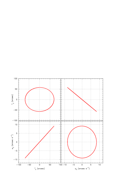
Figure 7: A typical evolution pattern for inertial rates and error angles for $\xi=10$ degrees. The two graphs in the upper right and lower left corners show the almost perfect relations between rates and error angles.

Substituting equations (50) and (51) in equation (49), we find

$$A_{x}=a_{y}/\bar{\omega}_{z} A_{y}=a_{x}/\bar{\omega}_{z},$$ ,

$$C_{x}=C_{1} B_{y}={(b_{x}-b_{y})\over 2\bar{\omega}_{z}}+C_{1},$$ ,

$$B_{x}=C_{2} C_{y}=C_{2},$$ ,

$$D_{x}=\frac{\omega_{2}(\gamma/f_{1}-\gamma)}{\bar{\omega}_{z}(1-\gamma^{2})} D_{y}=\frac{\omega_{1}(f_{2}-1)}{\bar{\omega}_{z}(1-\gamma^{2})},$$ ,

$$E_{x}=\frac{\omega_{1}(\gamma/f_{1}-\gamma)}{\bar{\omega}_{z}(1-\gamma^{2})} E_{y}=-\frac{\omega_{2}(f_{2}-1)}{\bar{\omega}_{z}(1-\gamma^{2})},$$ ,

$$F=\frac{-(b_{x}+b_{y})}{2},$$ (52)

where $C_{1}$ is a constant, depending on the choice of the reference position of the satellite’s $z$-axis. If $(T_{x,0},T_{y,0})$ are the Tait-Bryan angles at time zero, then for $\xi=0$ the following relations are obtained:

$$T_{x,0} = {a_{y}\over\bar{\omega}_{z}}+C_{1}+\frac{\omega_{2}(\gamma/f_{1}-\gamma)}{\bar{\omega}_{z}(1-\gamma^{2})},$$

$$T_{y,0} = {a_{x}\over\bar{\omega}_{z}}+C_{2}+\frac{\omega_{1}(f_{2}-1)}{\bar{\omega}_{z}(1-\gamma^{2})},$$ (53)

where $a_{x}$ and $a_{y}$ are relatively small with respect to the last terms. It is possible to choose the reference position for the Tait-Bryan angles such that $C_{1}$ and $C_{2}$ are equal to zero. This reduces the description of the motion of the satellite $z$-axis to a simple ellipse in the $(T_{x},T_{y})$ plane.

The coefficient for $F$ is a potential source of instability. An evaluation of the expected value of $F$, using equation (43), gives

$$F=\frac{-z_{0}G\sin 2\xi}{2I^{\prime}_{zz}\bar{\omega}_{z}}{\cal F}.$$ (54)

Using the input parameters specified in Section A.1 shows that the effect is quite small. From the values given we estimate a maximum drift of $166\times\sin 2\xi$ arcsec over a 1 hour period. With $\xi$ having a maximum value of 10 degrees, this is noticeable at the resolutions used by the Planck instruments.

It can be verified that for $\xi=0$ and $B=C_{1}=C_{2}=0$, and a fixed value of $\bar{\omega}_{z}$, linear relations exist between $T_{x}$ and $\omega_{y}$ and between $T_{y}$ and $\omega_{x}$. The ratios are

$$R_{1}\equiv {T_{x}-a_{y}/\bar{\omega}_{z}\over\omega_{y}}= \frac{1}{\bar{\omega}_{z}}\frac{1-f_{1}}{1-\gamma^{2}},$$

$$R_{2}\equiv {T_{y}-a_{x}/\bar{\omega}_{z}\over\omega_{x}}= \frac{-1}{\bar{\omega}_{z}}\frac{1-f_{2}}{1-\gamma^{2}}.$$ (55)

These relations, shown in Fig. 7, get only slightly disturbed by non-zero values for the solar aspect angle. They show that the satellite dynamics is dominated by the effects of the residual velocities around the $x$ and $y$ axes.

A.7 Numerical integration of the attitude model

Numerical integration of the Euler equation and the resulting rates can be performed without any of the approximations made in the analytic model; this provides a useful cross check on the analytic results. The integration over the Euler equation requires a set of inertial rates at the starting time. These have been chosen such that they represent the nominal rates: zero in $\omega_{x}$ and $\omega_{y}$, 6 degrees per second in $\bar{\omega}_{z}$. At time-steps of 0.01 s the torque acting on the satellite is developed, as well as the crossproducts of the rates ${\textbf{{I}}}^{-1}\omega\times{\textbf{{I}}}\omega$. This integration provides a record of the inertial rate development.

Similarly, the integration over the Tait-Bryan angles requires an assumption about the starting values. For $T_{x}$ and $T_{y}$ equation (53) is used to calculate the starting values, with $C_{1}=C_{2}=0$, while the $T_{z}$ starting value is set to zero.

A.7.1 Comparison with the analytic results

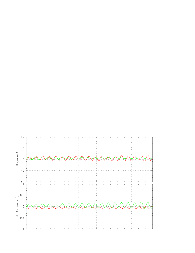
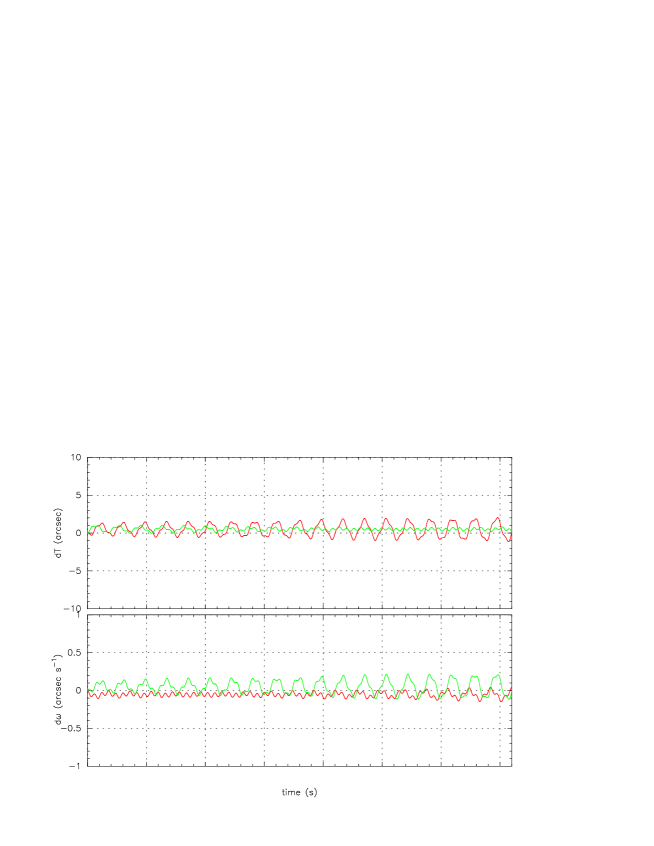
Figure 8: The differences between rates and error angles around the $x$ and $y$ axes as obtained from analytic modelling and from numerical integration. Top two graphs: a one-hour scan with $\xi=0$; bottom two graphs: $\xi=10$ degrees. The two curves in each graph show the variations for the $x$ and $y$ axes.

The results of the analytic approximation are compared with the numerical integrations in Fig. 8. These comparisons show that over a one-hour period the analytic approximation adds noise at a level of a few arcsec to the more accurate numerical integration. The main component of the noise originates from ignoring the $I^{\prime}_{xy}$ term in the development of equation (31). Including this term affects the amplitudes $\omega_{1}$ and $\omega_{2}$, and adds to these a small time-dependent term, which can, if necessary, also be estimated analytically. However, these corrections appear to be insignificant for Planck. The positional error in the analytic model is of the order of a few arcsec, which again is insignificant for Planck.

Given this level of agreement between the analytic and numerical models, it will be sufficient for the Planck simulations to use the analytic model, and to simulate only the initial conditions for a scan. In the same way, the conditions during re-positioning of the $z$-axis can be simulated. The simulations, as well as the analytic model, show that a solar aspect angle of $10^{\circ}$ or less has very little influence on the satellite’s attitude, unless this is examined at accuracies much higher than those required for Planck.

Appendix B Projections on the reference circle

In this appendix we describe the transformations for positions and rates from a system in which the spin axis describes a nutation ellipse in the satellite reference frame to a reference circle with its axis at the centre of this ellipse.

For $\xi=0^{\circ}$, the nutation ellipse is described in the satellite reference system by

$$T_{x} \approx A_{x}+D_{x}\cos\bar{\omega}_{z}\gamma t+E_{x}\sin\bar{\omega}_{z}\gamma t$$

$$T_{y} \approx A_{y}+D_{y}\cos\bar{\omega}_{z}\gamma t+E_{y}\sin\bar{\omega}_{z}\gamma t,$$ (56)

with the coefficients as defined in equation (51). In equation (44) it can in addition be assumed that $(\omega_{x,0},\omega_{y,0})$ are by far the dominant coefficients in $(\omega_{1},\omega_{2})$. This also implies that the coefficients $(A_{x},A_{y})$ will be relatively small with respect to $(\omega_{1},\omega_{2})$, so that we are left with

$$\omega_{x} \approx \omega_{x,0}\cos(\bar{\omega}_{z}\gamma t)-\frac{f_{1}}{\gamma}\omega_{y,0}\sin(\bar{\omega}_{z}\gamma t),$$

$$\omega_{y} \approx \omega_{y,0}\cos(\bar{\omega}_{z}\gamma t)+{\gamma\over f_{1}}\omega_{x,0}\sin(\bar{\omega}_{z}\gamma t),$$

$$T_{x} \approx R_{1}\bigl{[}\omega_{y,0}\cos(\bar{\omega}_{z}\gamma t)+{\gamma\over f_{1}}\omega_{x,0}\sin(\bar{\omega}_{z}\gamma t)\bigr{]},$$

$$T_{y} \approx R_{2}\bigl{[}\omega_{x,0}\cos(\bar{\omega}_{z}\gamma t)-{f_{1}\over\gamma}\omega_{y,0}\sin(\bar{\omega}_{z}\gamma t)\bigr{]},$$ (57)

where $R_{1}$ and $R_{2}$ are functions of $f_{1}$, $f_{2}$ and $\bar{\omega}_{z}$, as defined in equation (55), and $\gamma=\sqrt{f_{1}f_{2}}$ as defined in Section A.3. By choosing a suitable reference time $t_{0}$ equation (57) can be written as

$$\omega_{x} \approx \omega_{x,0}\cos\bigl{[}\bar{\omega}_{z}\gamma(t-t_{0})\bigr{]},$$

$$\omega_{y} \approx {\gamma\over f_{1}}\omega_{x,0}\sin\bigl{[}\bar{\omega}_{z}\gamma(t-t_{0})\bigr{]},$$

$$T_{x} \approx R_{1}{\gamma\over f_{1}}\omega_{x,0}\sin\bigl{[}\bar{\omega}_{z}\gamma(t-t_{0})\bigr{]},$$

$$T_{y} \approx R_{2}\omega_{x,0}\cos\bigl{[}\bar{\omega}_{z}\gamma(t-t_{0})\bigr{]},$$ (58)

The mean spin axis is assumed to be a fixed point in space, in the centre of the ellipse described by $(T_{x},T_{y})$, and the spin velocity is assumed to be the nominal spin velocity, $\omega_{z}=\bar{\omega}_{z}$. The offset angles can be defined with respect to a fixed reference system relative to the mean spin axis:

$$T_{x}^{\prime} = T_{x}\cos\psi-T_{y}\sin\psi,$$

$$T_{y}^{\prime} = T_{x}\sin\psi+T_{y}\cos\psi.$$ (59)

The angle $\psi$ is measured on the ring from its crossing of the reference circle (see Fig. 1). A point on the ring is given by the direction cosines

$$O_{i}=\left[\matrix{\cos\psi\sin\alpha\cr\sin\psi\sin\alpha\cr\cos\alpha}\right],$$ (60)

where $\alpha$ is the opening angle for the reference circle. The offset angles $(T_{x}^{\prime},T_{y}^{\prime})$ create small offsets in the actual angles $(\psi,\alpha)$ for a measurement. We ignore the very small rotation over $T_{z}$. The rotations over $T_{x}^{\prime}$ and $T_{y}^{\prime}$ distort equation (60)

$$O_{i}=\left[\matrix{\cos\psi\sin\alpha+T_{y}^{\prime}\cos\alpha\cr\sin\psi\sin\alpha-T_{x}^{\prime}\cos\alpha\cr\cos\alpha+T_{x}^{\prime}\sin\alpha\sin\psi-T_{y}^{\prime}\sin\alpha\sin\psi}\right],$$ (61)

which can also be expressed as

$$O_{i}=\left[\matrix{\cos\psi\sin\alpha+\Delta\alpha\cos\alpha\cos\psi-\Delta\psi\sin\alpha\sin\psi\cr\sin\psi\sin\alpha+\Delta\alpha\cos\alpha\sin\psi+\Delta\psi\sin\alpha\cos\psi\cr\cos\alpha-\Delta\alpha\sin\alpha}\right].$$ (62)

From these relations the expressions for $(\Delta\psi,\Delta\alpha)$ in terms of $(T_{x}^{\prime},T_{y}^{\prime})$ follow:

$$\Delta\psi = (-T_{x}^{\prime}\cos\psi-T_{y}^{\prime}\sin\psi)/\tan\alpha,$$

$$\Delta\alpha = -T_{x}^{\prime}\sin\psi+T_{y}^{\prime}\cos\psi.$$ (63)

Substituting equation (59) we find

$$\Delta\psi = -T_{x}/\tan\alpha,$$

$$\Delta\alpha = +T_{y}.$$ (64)

With an opening angle $\alpha$ of 80 to 85 degrees, the effect of the spin-axis wobble on the scan phases is very small. The maximum amplitude is expected to be less than 0.12 arcmin. This may be visible, though, in the star mapper data. The effect of $T_{x}$ on the orientation of the focal plane is even smaller.

The $\alpha$ variations can be relevant for the high-frequency detectors. A change in position of the beam by $\pm 0.75$ arcmin for a point source close to the steepest slope of the beam will create significant variations in the signal over a TOP. If the wobble parameters can be reconstructed from the star mapper data, then some of this variation may be accounted for in the reductions.

References

- [Baccigalupi et al.2000] Baccigalupi C. et al., 2000, MNRAS, 318, 769
- [Bierman 1977] Bierman G. J., 1977, Factorisation methods for discrete sequential estimation. Academic Press, New York
- [Brink & Satchler 1993] Brink D. M., Satchler G. R., 1993, Angular Momentum, 3rd ed. Clarendon Press, Oxford
- [Cayon et al. 2000] Cayon L., Sanz J. L., Barreiro R. B., Martínez-González E., Vielva P., Toffolatti L., Diego J. M., Argüeso F., 2000, MNRAS 315, 757
- [Challinor et al. 2000] Challinor A., Fosalba P., Mortlock D., Ashdown M., Wandelt B, Górski K., 2000, Phys. Rev. D 62, 123002
- [Challinor et al. 2002] Challinor A. D., Mortlock D. J., van Leeuwen F., Lasenby A. N., Hobson M. P., Ashdown M. A. J., Efstathiou G. P., 2001, MNRAS, in press (astro-ph/0112277)
- [Crittenden 2000] Crittenden R. G., 2000, Astro. Lett. and Communications, 37, 337
- [Crittenden & Turok 1998] Crittenden R. G., Turok N. G., 1998, ApJ, submitted (astro-ph/9806374)
- [Delabrouille, Górski & Hivon 1998] Delabrouille J., Górski K., Hivon E., 1998, MNRAS, 298, 445
- [ESA 1989] ESA, 1989, SP1111, The Hipparcos mission, Volume III
- [ESA 1997] ESA, 1997, SP1200, The Hipparcos and Tycho Catalogues, Volume 3
- [Górski 1994] Górski K. M., 1994, ApJ, 430, L85
- [Górski 1999] Górski K. M., 1999, in Banday A. J., Sheth R. K., da Costa L. N., eds, Evolution of large scale structure: from recombination to Garching. PrintPartners, Ipskamp, N. D., 37
- [Hobson et al. 1998] Hobson M. P., Jones A. W., Lasenby A. N., Bouchet F. R., 1998, MNRAS, 300, 1
- [Kovalevsky et al. 1997] Kovalevsky J. et al., 1997, A&A, 323, 620
- [van Leeuwen 1997] van Leeuwen F., 1997, Spac. Sci. Rev., 81, 201
- [Lindegren 1979] Lindegren L., 1979, in Prochazka F. V., Tucker R. H., eds, Proc. IAU Colloquium 48, Modern Astrometry. University Observatory Vienna, 197
- [Mortlock, Challinor & Hobson 2001] Mortlock D. J., Challinor A. D., Hobson M. P., 2002, MNRAS, in press
- [Prunet et al. 2001] Prunet S., Teyssier R, Scully S. T., Bouchet F. R., Gispert R., 2001, A&A in press
- [Revenu et al. 2000] Revenu B., Kim A., Ansari R., Couchot F., Delabrouille J., Kaplan J., 2000, A&A 142, 499
- [Sanz et al. 2001] Sanz J. L., Herranz D., Martínez-Gónzalez E., 2001, ApJ, 552, 484
- [Spence 1978] Spence C., 1978, in Wertz J., ed., Spacecraft attitude determination and control. Reidel, Dordrecht, 566
- [Stolyarov et al. 2002] Stolyarov V., Hobson M. P., Ashdown M. A. J., Lasenby A. N., 2002, MNRAS, in press
- [Sunyaev & Zeldovich 1980] Sunyaev R. A., Zeldovich Ya. B., 1980, MNRAS, 190, 413
- [Wandelt & Górski 2001] Wandelt B., Górski K. W., 2001, Phys. Rev. D, 63, 123002
- [Wandelt, Hivon & Górski 2001] Wandelt B., Hivon E., Górski K. M., 2001, Phys. Rev. D, in press