Solar Magnetic Field Studies Using the 12-Micron Emission Lines. IV. Observations of a Delta-Region Solar Flare

Abstract

We have recently developed the capability to make solar vector (Stokes IQUV) magnetograms using the infrared line of MgI at 12.32 µm. On 24 April 2001, we obtained a vector magnetic map of solar active region NOAA 9433, fortuitously just prior to the occurrence of an M2 flare. Examination of a sequence of SOHO/MDI magnetograms, and comparison with ground-based H-alpha images, shows that the flare was produced by the cancellation of newly emergent magnetic flux outside of the main sunspot. The very high Zeeman-sensitivity of the 12 µm data allowed us to measure field strengths on a spatial scale which was not directly resolvable. At the flare trigger site, opposite polarity fields of $2700$ and $1000$ Gauss occurred within a single $2$ arc-sec resolution element, as revealed by two resolved Zeeman splittings in a single spectrum. Our results imply an extremely high horizontal field strength gradient ($5$ G/km) prior to the flare, significantly greater than seen in previous studies. We also find that the magnetic energy of the cancelling fields was more than sufficient to account for the flare’s X-ray luminosity.

1 Introduction

Solar flares are believed to be powered by the release of magnetic energy, but the details of the process are not understood. Flare-related changes in magnetic configurations of active regions have long been sought, without clear success. However, recent observations using ground-based (Cameron and Sammis, 1999; Harvey, 2001) and space-borne magnetographs (Kosovichev and Zharkova, 1999, 2001) are beginning to show clear signatures of magnetic energy release, temporally coincident with large flares. It has long been known that small to moderate flares can occur where newly-emergent flux becomes abutted against its opposite polarity (Martin et al., 1984) and is cancelled, presumably by reconnection. Flux-cancellation represents one obvious type of flare-related magnetic change, but it is also believed that flux cancellation can trigger the release of magnetic energy stored over larger volumes (Priest, 1984). The derivation of the magnetic energy from observations requires accurate measurement of the magnetic field strength, and conventional magnetographs can give large errors in field strength. Because Zeeman splitting for visible-region lines is less than the intrinsic line width, it can be difficult to discriminate between a strong field having a small filling factor, and a much weaker field with unit filling factor, and these two cases can represent vastly different magnetic energies.

In recent years, infrared (IR) lines have been increasingly used (Meunier et al., 1998), because they can exhibit resolved Zeeman splitting, giving the field strength independent of filling factor for fields stronger than some limit (typically $\sim 400$ Gauss at 12 µm). We have been developing instrumentation to make vector field maps (Stokes $IQUV$) of solar active regions using the far-IR line of MgI at 12.32 µm. One of our vector field maps was fortuitously made just prior to the occurrence of an M2 flare initiated by flux cancellation. Our data have insufficient temporal resolution to demonstrate a decrease in magnetic energy at the precise time of the flare. Nevertheless, we exploit the great Zeeman-sensitivity of these data to demonstrate that the flare began where the horizontal gradient in field strength was exceptionally large ($\gtrsim 5$ G/km), and that the magnetic energy in the immediate vicinity of the flux-cancellation site was more than ample compared to the flare’s X-ray luminosity.

2 Observations

We observed the largest sunspot in NOAA region 9433 on 23-25 April 2001, at the McMath-Pierce telescope of the National Solar Observatory on Kitt Peak. We used our cryogenic grating spectrometer, ‘Celeste’ mounted on top of the main spectrograph tank to take advantage of its ability to track the image rotation. Celeste achieves nearly diffraction-limited spectral and spatial resolution, and background-limited sensitivity. It uses a large echelle grating ($18\times 33$ cm²) to achieve a resolution of 0.04 cm^-1 on the 12.32 µm line, corresponding to a magnetic resolution of $\sim 400$ Gauss. (We define magnetic resolution as the minimum field strength difference which becomes visible as distinct Zeeman splittings in a single spectrum. See Deming et al. (1991) for a discussion.) As shown in Figure 1, the beam from the telescope is collimated, passed through the polarimeter optics, and is focused into Celeste. In the spectrometer, the beam passes through a filter wheel, and forms an image at a $2$ arc-sec $\times\ 2.3$ arc-minute slit. The beam is then collimated by internal Cassegrain optics, diffracted at the grating, and refocused at the detector array. The array is a $128\times 128$ blocked-impurity-band device, with 75 µm pixels, giving 1 arc-sec per pixel scale, double-sampling the $\sim 2$ arc-sec telescope diffraction image. The spectrometer is housed in a liquid-Helium dewar.

We record full vector magnetograms. The mapping process consists of stepping the solar image using a limb-guider, and cycling through the Stokes parameters sequentially at each spatial position. The process is performed at a steady cadence under computer control. In the polarimeter optics the beam transits a 1/4-wave plate, a 1/2-wave plate, and a chopping linear polarizer. By selecting combinations of rotation angles for the two waveplates, followed by the chopping polarizer, we measure $I$, $Q$, $U$, and $V$. We use a double-differencing technique to subtract unpolarized light, and to cancel any imbalance between the two polarizer positions. Beginning with the waveplate settings for $Q$, the two positions of the chopping polarizer give spectra of $I_{u}+Q$ and $I_{u}-Q$. The next waveplate setting gives $I_{u}-Q$ and $I_{u}+Q$ (reverses the sign) for the two polarizer positions. The sum of these yields $I_{u}$ and the differences yield $Q$. This cycle is repeated for $U$ and $V$. Stokes $I$ is calculated from $I^{2}=Q^{2}+U^{2}+V^{2}$. Thus all four Stokes parameters, and also the unpolarized spectrum $I_{u}$ are derived from the measurements. This method of observing the 12.32 µm line Stokes parameters is an adaptation and extension of the method pioneered by Hewagama et al. (1993).

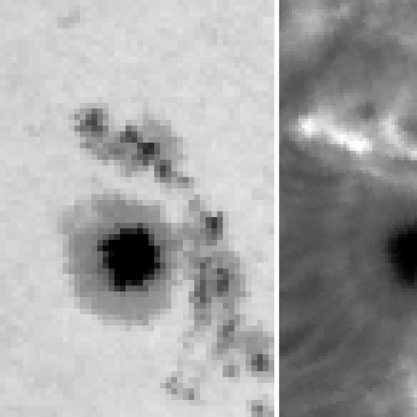
Figure 2: MDI magnetogram (upper left, 17:36 UT), white light (lower left, 17:18 UT, and BBSO H-alpha (lower right, 17:58 UT) images of the main spot in NOAA 9433 taken just prior to our 12 µm IQUV data. The upper right panel repeats the MDI magnetogram, and superposes arrows which indicate the direction of flux transport (length of the arrows has no significance). Moving positive flux (brighter areas) diverges from the spot marked with ‘+’. The two boxed areas indicate ‘delta regions’ having opposite polarity in close proximity; the upper we designate as region 1, and the lower right one as region 2. The area and orientation of these images were adjusted to match our 12 µm data (Figure 4). The line marked ‘3’ indicates the slit position corresponding to Figure 3; the 12 µm slit was oriented vertically, and stepped to the right.

Figure 2 shows a SOHO Michaelson Doppler Imager (MDI) magnetogram and continuum image of the observed spot, as well as an H-alpha image from the Big Bear Solar Observatory (BBSO). The immediate vicinity of the observed (positive polarity) spot consisted of smaller pores of negative polarity. We inspected a sequence of MDI magnetograms from $10$ hours before to several hours after our observations. This showed that newly-emergent positive polarity flux was diverging from the point marked with ‘+’ on Figure 2. Positive flux was also flowing radially outward from the main spot, so flux emergent from the ‘+’ point was forced into close coincidence with the small negative polarity spots in the two regions outlined with boxes on the upper right panel of Figure 2. Opposite polarity umbrae existing within a single sunspot are conventionally termed a ‘delta configuration.’ Although the opposite polarity regions observed here are not mature umbrae, they do have field strengths attaining umbral values ($\gtrsim 2000$ Gauss). We therefore refer to these two locations where opposite polarities are in contact as ‘delta regions’.

During our 24 April IQUV mapping sequence an M2-class X-ray flare occurred in the region. Relevant timing data for the flare and our mapping sequence are given in Table 1. H-alpha sequences recorded at BBSO, and the H-alpha video recorded on the Razdow telescope at NSO Kitt Peak, show a general brightening in the delta regions surrounding the spot (see Figure 2, lower right panel), which increased gradually in the hours before the flare. The flare began with a sudden additional H-alpha brightening in delta region 2, which spread rapidly to region 1. Clouds interfered toward the end of our mapping sequence, but fortunately this happened after the flare onset, and after the most significant portions of the 12 µm magnetogram were complete.

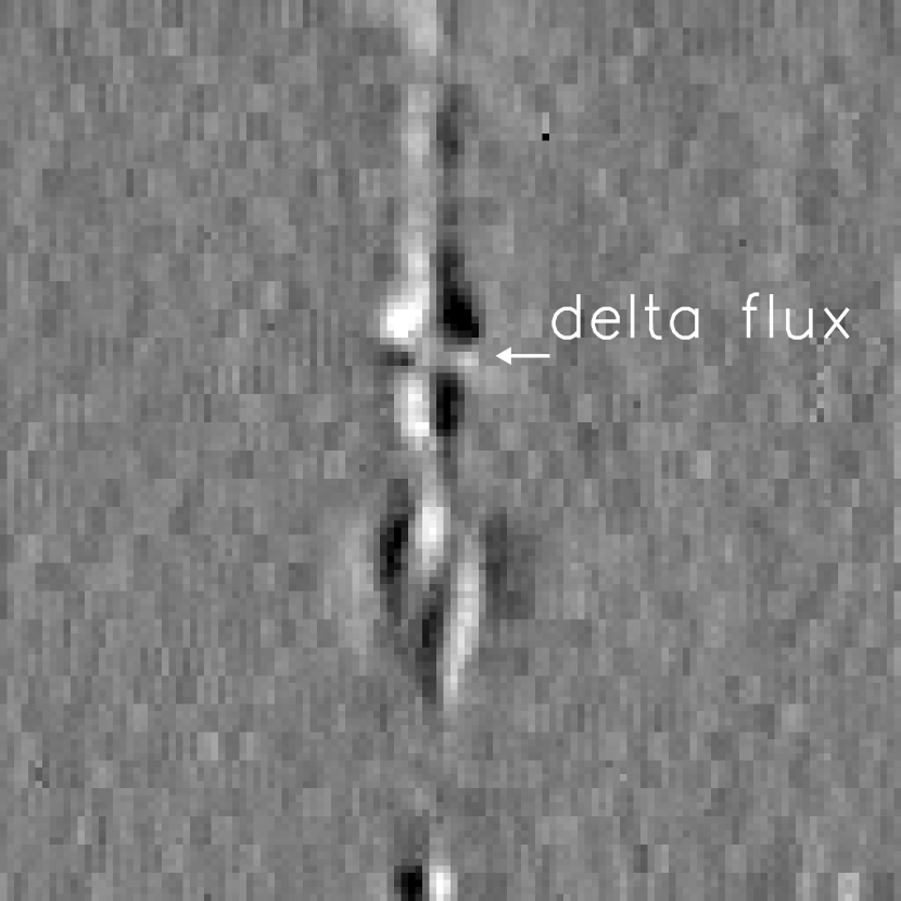
Figure 3: Sample Stokes images for a slit position cutting through the penumbra of the main spot, and into the delta configuration. The top image is the total linear polarization, i.e. $(Q^{2}+U^{2})^{1/2}$ (we measure Q and U separately), and the bottom image is Stokes-V. The reversal of polarity in the delta region number 1 (see Figure 2) is marked by an arrow. A mark on Figure 2 identifies the location of the slit for these sample profiles.

Figure 3 shows an example of transverse ($(Q^{2}+U^{2})^{1/2}$, upper panel) and longitudinal field (Stokes-V) images made during our mapping sequence. These are detector-plane images made at the slit position marked on Figure 2. One dimension is spatial, and cuts through the main spot, extending into delta region number 1. The other dimension is frequency in wavenumbers, and shows the familiar Zeeman patterns for circular and linear polarization as image brightness variations. Because of the large splitting in this line, the magnitude of the linear polarization is comparable to the circular polarization.

3 Results

The data shown here are among the first 12 µm polarization maps ever observed for a solar active region. Given the large Zeeman sensitivity, and greater height of formation for this line, new features are to be expected.

Prior to showing the 12 µm magnetic maps, we point out some interesting aspects of the sample Stokes profiles illustrated on Figure 3. Between $\sim 30$ and $\sim 70$ arc-sec, the slit crosses the penumbra of the main spot. The Stokes-V profiles show large apparent Doppler shifts, which reverse as the slit passes the center of the spot. Since this sunspot was close to disk center (N18E06), the direction of these flows is primarily upward and downward on opposite sides of the spot. This flow pattern is not uniquely related to the flare, because it was also observed on April 23 and 25. The apparent magnitude of the flow is supersonic, $\sim 20$ km/sec. Although we have observed several sunspots, this is the first instance of such large apparent Doppler shifts. Note that the transverse field does not exhibit these shifts. Although our method does not measure linear polarization strictly simultaneously with circular, the same properties (Doppler shifts in V, and not in Q and U) are seen over extended regions of this sunspot on all days. We tentatively interpret this effect as resulting from the ‘fluted’ nature of the sunspot penumbra (Title et al., 1993), wherein field lines of drastically different inclination can co-exist at the same general location. Evidently we are seeing high-velocity flows along the field lines which are nearly vertical, while simultaneously seeing linear polarization from field lines which are nearly horizontal. In comparison to most lines used for magnetograms, the 12 µm line is formed significantly higher (near $\sim 400$ km, Chang et al. (1991); Carlsson et al. (1992)) which may exaggerate effects due to sunspot activity and fluting.

Near $\sim 85$ arc-sec the slit crosses delta region 1 (compare Figure 2). The field in this region is nearly all in Stokes-V; the transverse component is negligible. Again, since this active region was close to disk center, the fields in the delta region are nearly vertical, i.e. directed radially outward from sun center. The field strength, as seen by the splitting in Stokes-V, is at least as large as the strongest penumbral field in the main spot (the 12 µm line disappears in sunspot umbrae, so we cannot compare directly with the main spot umbral field). In delta region 2 (not illustrated) some linear polarization signal does appear, but the fields are still primarily vertical, and their field strengths are even greater.

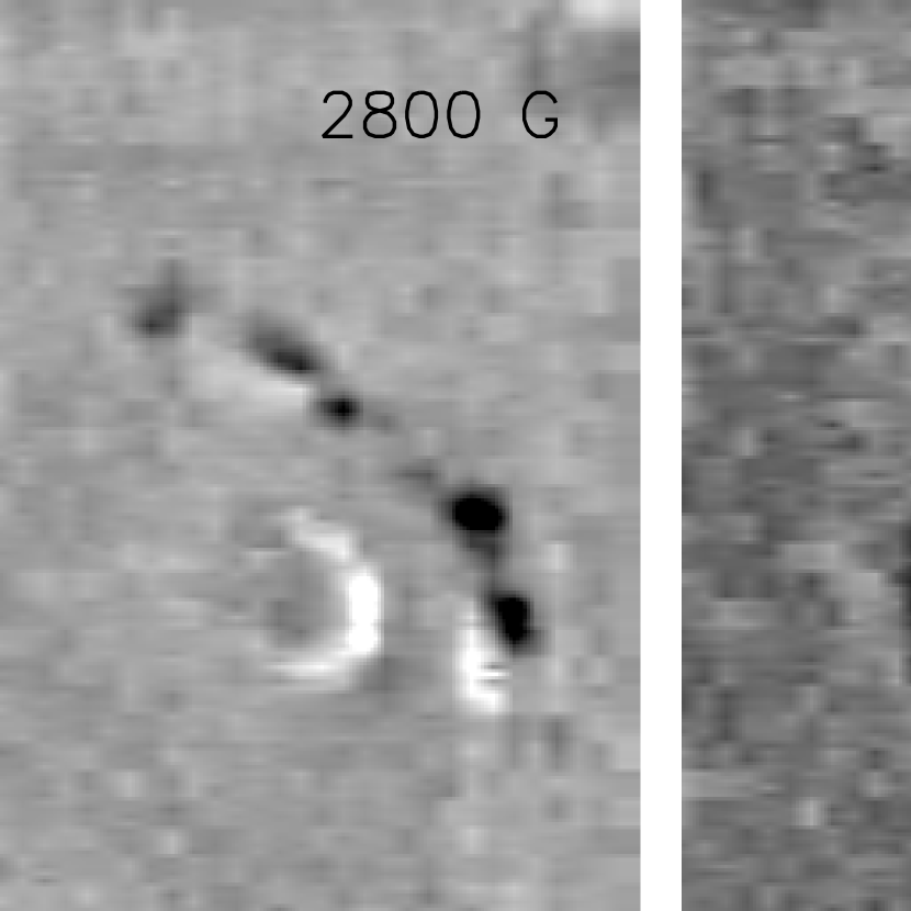
Figure 4: 12 µm magnetograms made by ‘slicing’ the Stokes-V image cube at increasing values of the field strength. Compare to the MDI magnetogram (Fig 2). Brightness indicates the polarity and intensity of the line emission at the splitting value corresponding to the given field strength (positive polarity is bright, negative is dark). The intensity scale of each image is normalized separately, for clarity of display. These magnetograms were obtained by scanning the Celeste slit (vertical on this representation) from left to right. The Stokes-V profile in the region marked by a circle on the 2100 Gauss panel is plotted on Figure 5.

Since the delta region fields are represented primarily in Stokes-V, we use Stokes-V to illustrate our magnetic map of this region. In each spectrum, we determined the zero-crossing wavelength of the V-profiles (using spline interpolation), and we ‘folded’ the profiles about their zero-crossing point. Since our Stokes-V profiles are not systematically asymmetric, the folding increases the signal-to-noise level without losing physical information. Because the Zeeman sensitivity of this line is so large, we can show magnetograms at a given field strength. For example, only weak fields contribute near the center frequency of the line, because the large Zeeman splitting from strong fields displaces their Stokes-V components away from line center. So the third dimension of our magnetic map is field strength. Figure 4 shows our magnetogram ‘sliced’ at 350, 700, 1400, 2100, 2800, and 3900 Gauss. Near 80 arc-sec on the horizontal scale the data were affected by clouds, but we verified that the important delta region 2 near 70 arc-sec was unaffected.

4 Discussion

The 350 Gauss panel of Figure 4 shows a noticeably more ‘diffuse’ appearance than the panels at higher field strengths. This shows that weak fields are present in active regions. They are broadly distributed, in contrast to strong fields - which concentrate at specific locations. A large fraction of the weak field component is due to the sunspot ‘canopy’, which can be seen as the extended region of positive polarity most obvious in Stokes-V on the side of the sunspot toward disk center (compare Figure 2). We have previously described a prominent sunspot canopy observed in the 12.32 µm line (Jennings et al., 2001).

The sunspot penumbral field shows a ring-like morphology, which of course reflects the fact that the single field strength in each panel is found at only a particular radius from the spot center. With increasing field strength, the width and radius of the ring decrease. At the largest field strength (3900 Gauss), the polarity of the sunspot field seems to reverse. We have observed this effect in several sunspots, and it is certainly not an observational artifact. However, it does not represent an actual polarity reversal. Recall that this emission line is flanked by a broad, shallow, absorption trough (Chang and Schoenfeld, 1991). At large distances from line center, the sunspot Stokes-V profile is dominated by the relatively low-amplitude V signal from the absorption trough, which accounts for the apparent polarity reversal. In principle, this effect conveys information on the height gradient of field strength, since the absorption is formed deeper than the emission. However, a quantitative interpretation is beyond the scope of this paper.

The MDI whole-disk magnetogram at 17:36 UT registers peak field strengths of $\sim 250$ and $\sim 500$ Gauss for the positive polarity fields in delta regions 1 and 2 respectively. In contrast, the 12 µm data show that these regions are not even prominent in positive polarity until the field strength exceeds $700$ Gauss, with significant intensity being recorded even at $2800$ Gauss. Evidently the fields are not resolved at the MDI whole disk resolution of $2$ arc-sec. Although our spatial resolution was also $2$ arc-sec, the very large Zeeman splitting in the 12 µm line permits us to measure true field strengths without spatially resolving the fields. In both delta regions 1 and 2 the average strength of the positive polarity fields is $\sim 2000$ Gauss, but in delta region 2 (where the flare was triggered), the distribution of field strengths extends to greater values than in region 1. This is noticeable in the 3900 gauss panel, where a trace of delta region 2 can still be discerned. Moreover, these fields are in quite close proximity to the small negative polarity pores, producing exceptionally large field strength gradients. Figure 5 shows the Stokes-V profile at the point in delta region 2 where opposite polarities are in contact (marked by the circle on the 2100 Gauss panel). Within the $2$ arc-sec spatial resolution element, two distinct Zeeman splittings are seen: a 2700 Gauss splitting at positive polarity, and 1000 Gauss at negative polarity. These splittings are marked on Figure 5. We contemplated alternative interpretations of this complex Stokes-V profile, which might lessen the necessity for strong opposite-polarity fields in close spatial coincidence. However, alternate interpretations are difficult to reconcile with the Stokes-V profiles in immediately adjacent regions, which support the picture of strong fields in both polarities.

This large field strength difference in such close proximity requires a horizontal field gradient of $\sim 5$ G/km. To our knowledge, this is the largest horizontal gradient ever observed on the Sun, and suggests reconnection at this site, at or near the temperature-minimum height. In their study of upper-photospheric reconnection, Litvinenko and Martin (1999) remark that ‘the local field cannot be…measured directly.’ The high magnetic resolution afforded by the 12 µm line indeed makes such a measurement possible, and the height of line formation is well matched to the temperature-minimum region where the electrical resistivity is maximum. We therefore point out the significant diagnostic potential of the 12 µm line in studies of photospheric reconnection.

Other investigators find high field strength gradients at flaring sites, but less than we infer here. Kosovichev and Zharkova (2001) found a gradient of $1.3$ G/km for the X5.7 ‘Bastille Day’ flare; our results for a significantly weaker flare suggest that conventional magnetographs (even space-borne ones such as SOHO/MDI) underestimate the field strength gradients. If so, they probably also underestimate the magnitude of magnetic energy release inferred from observed changes in the fields.

Our results have significant implications for the magnetic energy available locally (i.e., in the flux-cancellation region of the mid- to upper photosphere) to power this flare. The total magnetic energy is proportional to the volume integral of $\frac{B^{2}}{8\pi}$ (Chandrasekhar, 1961). We estimate this quantity directly from the Stokes-V profiles:

$$E_{tot}=\frac{\delta H}{8\pi}\epsilon\sum B^{2}f_{B}dA$$ (1)

where the volume integral is approximated as a discrete sum over field strengths within a spatial resolution area $dA$, times a layer thickness $\delta H$. $\epsilon$ is the fraction of the atmosphere which is magnetic, i.e. a filling factor. We constrain $\epsilon>0.15$ by comparing the MDI and 12 µm field strengths. The factor $f_{B}$ expresses the fraction of the magnetic atmosphere which exhibits field strength $B$. The essential advantage of a strongly-split infrared line is that we can infer $f_{B}$ as proportional to the amplitude of the Stokes-V profile at each splitting (i.e., field strength) value. (In so doing we assume that the line formation mechanism for the 12.32 µm transition is independent of field strength.) Moreover, because the 12 µm line is formed in the temperature minimum region, $\sim 400$ km above the photosphere (Chang et al., 1991; Carlsson et al., 1992), we know that $\delta H>400$ km. On this basis we find that the total ‘local’ magnetic energy of region 1 was $>3\times 10^{22}$ Joules, and of region 2, $>4.5\times 10^{22}$ Joules. Using the single-value MDI field strengths with unit filling factor gives $3.5\times 10^{20}$ and $6\times 10^{21}$ Joules for regions 1 and 2 respectively. By comparison, the X-ray luminosity of the flare was $3\times 10^{21}$ Joules. As is well known, only a fraction of the total magnetic energy is available to a flare (Low and Lou, 1990), and the flare’s total luminosity will of course be greater than the energy measured in the GOES X-ray bands (Table 1). Hence the MDI energies are uncomfortably small, but the 12 µm field strengths indicate an ample local resevoir of magnetic energy. A conventional view is that cancelling magnetic flux simply triggers the release of magnetic energy stored in much larger volumes. While this may actually happen for many of the largest flares, our results imply that sufficient energy was available to power this M2 flare ‘locally’, without invoking the release of magnetic energy from much larger volumes.

Figure 1: Optical layout used to measure Stokes $IQUV$ profiles at 12.32 µm.

Figure 5: Stokes-V profile for the specific location in delta region 2 (marked with a circle on Figure 4) where strong-field opposite polarities are in close coincidence. Two separate Zeeman splittings of 2700 and 1000 Gauss, with opposite polarities, are marked. Line center is at 811.58 cm^-1.

Table 1: Parameters for the Flare and 12 µm Map

Parameter
Flare Begin	18:04 UT
Flare Peak	18:12 UT
Flare End	18:17 UT
Flare X-ray Luminosity	$3\times 10^{21}$ Joules
12 µm Map Start	16:15 UT
12 µm Map End	18:52 UT

References

- Cameron and Sammis (1999) Cameron, R., and Sammis, I. 1999, ApJ, 525, L61
- Carlsson et al. (1992) Carlsson, M., Rutten, M. J., and Shchukina, N. G. 1992, A&A, 253, 567
- Chandrasekhar (1961) Chandrasekhar, S. 1961, Hydrodynamic and Hydromagnetic Stability, Dover Publications.
- Chang et al. (1991) Chang, E. S., Avrett, E. H., Mauas, P. J., Noyes, R. W., and Loeser, R. 1991, ApJ, 379, L79
- Chang and Schoenfeld (1991) Chang, E. S., and Schoenfeld, W. G. 1991, ApJ, 383, 450
- Deming et al. (1991) Deming, D., Hewagama, T., Jennings, D. E., and Wiedemann, G. 1991, in Solar Polarimetry, Proceedings of the Eleventh National Solar Observatory / Sacramento Peak Summer Workshop, L. J. November (ed), National Solar Observatory, Sunspot NM, p.341.
- Harvey (2001) Harvey, J. W., 2001, American Geophysical Union, Spring Meeting 2001, abstract SH22A-01
- Hewagama et al. (1993) Hewagama, T., Deming, D., Jennings, D. E., Osherovich, V., Wiedemann, G., Zipoy, D., Mickey, D. L., and Garcia, H. 1993, ApJS, 86, 313
- Jennings et al. (2001) Jennings, D. E., Deming, D., Sada, P. V., McCabe, G. H., and Moran, T. 2001, in Advanced Solar Polarimetry: Theory, Observation and Instrumentation, M. Sigwarth (ed), ASP Conference Series 236, 273
- Kosovichev and Zharkova (1999) Kosovichev, A. G., and Zharkova, V. V. 1999, Sol. Phys., 190, 459
- Kosovichev and Zharkova (2001) Kosovichev, A. G., and Zharkova, V. V. 2001, ApJ, 550, L105
- Litvinenko and Martin (1999) Litvinenko, Y. E., and Martin, S. F. 1999, Sol. Phys., 190, 45
- Low and Lou (1990) Low, B. C., and Lou, Y. Q. 1990, ApJ, 352, 343
- Martin et al. (1984) Martin, S. F., and 10 co-authors 1984, Adv. Space Res., 4, 61
- Meunier et al. (1998) Meunier, N., Solanki, S. K., and Livingston, W. C. 1998, A&A, 331, 771
- Priest (1984) Priest, E. R. 1984, Adv. Space Res., 4, 37
- Title et al. (1993) Title, A. M., Frank, Z. A., Shine, R. A., Tarbell, T. D., Topka, K. P., Scharmer, G., and Schmidt, W. 1993, ApJ, 403, 780