Determination of masses and other properties of extra-solar planetary systems with more than one planet

Abstract

Recent analysis of the Doppler shift oscillations of the light from extra-solar planetary systems indicate that some of these systems have more than one large planet. In this case it has been shown that the masses of these planets can be determined without the familiar ambiguity due to the unknown inclination angle of the plane of the orbit of the central star provided, however, that its mass is known. A method is presented here which determines also a lower limit to the mass of this star from these observations. As an illustration, our method is applied to the Keck and Lick data for GJ876.

1 Introduction

During the past six years a large number of extra solar planetary systems have been discovered by observations of Doppler shifted oscillations of the light emitted by the central star (Udry, 2000). Recent analysis of the data has shown that some of these systems have more than one Jupiter-size planet circulating the central star (Marcy,Fischer,Butler &Vogt, 2001). It is well known that when there is only a single planet an ambiguity occurs in the determination of the mass of this planet when the inclination angle of the plane of the orbit is not known. For systems with more than one sizable planet, however, it turns out that this ambiguity can be removed when the gravitational interaction between these planets is important to the evolution of the planetary orbits, as has been pointed out by Laughlin and Chambers (2001). By the equivalence principle this interaction is proportional to the mass of the planets, thus providing an additional dependence on these masses which is absent when there is only a single planet. In the case of multiple planets only approximate analytic solutions of the gravitational equations of motion exist, and one must resort to numerical integrations to analyze the data. In this paper we present a method based on such an integration to obtain the masses and other properties of the extra-solar planetary system. As an illustration we apply our method to the Keck and Lick data for GJ876 obtained by Marcy et. al. (2001). Some previous analyses of this data depended on the approximation that each of these planets is traveling on a Keplerian elliptical orbit with either constant orbital elements, Marcy et. al. (2001), or on variable orbital elements , Laughlin and Chambers (2001), although these latter authors have implemented also an exact numerical integration of the equations of motion . While we have been able to verify their results with our method, we have found a second solution which differs significantly from theirs. The value of the reduced chi-square of these two fits is of order 2.5 - 3, although the mean is approximately one, indicating that some fundamental physics in the analysis of the data has not been taken into account. Indeed, an additional source for velocity fluctuations in the light emitted by the central star may be due to the convective motion and turbulence of the chromosphere, which has been shown to be correlated to increase magnetic activity in some stars, Saar, Butler and Marcy (1998), Saar and Fischer (2000). An estimate of the magnitude of these fluctuations can be obtained from the requirement that the reduced chi-square be of order unity, as will be shown in section 3.

2 Method for analysis of extra-solar planetary data

Our starting point is to re-scale the gravitational equations of motion by introducing a length scale $l$ and time scale $\tau$ which satisfies the Kepler-Newton relation

$$\frac{l^{3}}{\tau^{2}}=Gm_{s},$$ (1)

where $m_{s}$ is the mass of the central star. This mass is taken as one of the parameters in a least-square fit to the data, while either $l$ or $\tau$ can be chosen as another parameter. In these rescaled variables the magnitude of the force per unit mass due to a planet with mass $m^{g}_{j}$ at a distance $r_{j}$ is is

$$(m^{g}_{j}/m_{s})(1/r_{j}^{2})$$ (2)

For clarity we have labeled this planetary mass with a superscript $g$ to indicate that we are referring here to the gravitational masses. On the other hand, by momentum conservation, the velocity of the central star is related to the velocities $v_{j}$ of $n$ planets according to the relation

$$\vec{v}_{s}=-\sum_{j=1}^{j=n}\frac{m^{i}_{j}}{m_{s}}\vec{v}_{j}+\vec{v}_{o}$$ (3)

which depends on the inertial masses $m^{i}_{j}$ of the planets which we label by the superscript $i$. Here, the velocity $v_{o}$ is proportional to the uniform velocity of the center of mass relative to the observer, and becomes another parameter in our fit. By the equivalence principle, the gravitational and inertial masses are equal, $m^{g}_{j}=m^{i}_{j}=m_{j}$, which implies that the same mass ratio $m_{j}/m_{s}$ appears in both this kinematical relation and in the dynamical interaction between planets, Eq. 2. This is the key which opens a new way to obtain these mass ratios in extra-solar planetary systems with more than one planet. According to our scaling, Eq. 1, the observed velocities are obtained by multiplying these velocities by a scale factor

$$V=\frac{l}{\tau}=(\frac{Gm_{s}}{\tau})^{(1/3)}$$ (4)

The observed Doppler variations, however, depend also on the inclination angle $i$ of the mean plane of the orbit of the star relative to the observer, and therefore the relevant scale for observations is the product $Vsin(i)$. Consequently, the independent parameters in a fit to the observations are the product $m_{s}sin^{3}(i)$ and the mass ratios $m_{j}/m_{s}$.

The additional parameters which are required to determine the evolution of the extra solar system are those parameters which determine the initial conditions, e.g. the position and velocities of each of the planets at the start of the observations, and the relative uniform velocity of the center of mass of the system. The initial velocity of the central star is then given by the conservation of momentum relation Eq. 3. A useful approach, currently in practice, is to parameterize the orbital elements of the initial osculating Keplerian ellipse for each planet. It must be remembered, however, that when interplanetary perturbations are important these orbital elements evolve in time. As will be shown below, some of these elements have periodic variations, while others change continuously. Hence, in general these initial parameters do not describe the mean properties of the system when interplanetary perturbations are important.

The values of the parameters are obtained by a least square fit to the data obtained by integrating numerically the gravitational equations of motions. In particular, we consider the dependence of this fit as a function of our parameter $m_{s}sin^{3}(i)$. According to Eqs. 3 and 4, when this parameter is increased above the value at which a minimum has been found, the planetary mass ratios $m_{j}/m_{s}$ are expected to decrease inversely with the cube root of $m_{s}sin^{3}$, in order to fit the observed velocity of the star. Hence, if the inter-planetary interactions are important the chi-square of the fit should increase; otherwise it approaches a constant. Correspondingly, when this parameter is decreased the chi-square also increases, because now the interplanetary interactions increases above their actual value. Since $sin(i)\leq 1$, the value of the parameter $m_{s}sin^{3}(i)$ at the minimum chi-square then gives a lower limit for the mass $m_{s}$. When this mass can also be obtained from the mass-luminosity relation, our method provides a novel check on the validity of this relation as well as on the self-consistency of the least-square fit.

3 Application to GJ 876

We illustrate our method by an application to the Keck and Lick data for the velocity modulations of GJ876 obtained by Marcy et al (2001). These authors have fitted their data assuming that there are two large planets orbiting the center of mass on Keplerian ellipses which have constant orbital elements, and they found that the periods were nearly in a 2:1 ratio. The occurrence of this resonance, however, indicates that the interactions between these planets cannot be neglected as was assumed originally. Recently, Laughlin and Chambers (2001) also fitted this data by integrating the equations of motion numerically, but we have found that their solution is not unique, and we present here another fit which gives planetary masses and other properties of the system which differ significantly from their results.

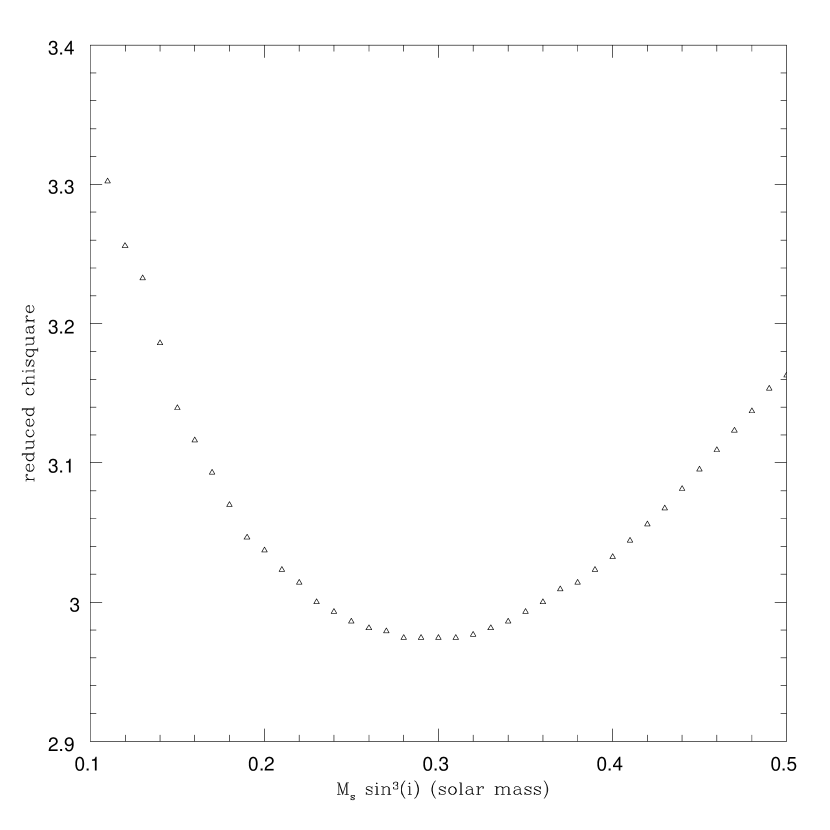
Figure 1: An eleven parameter least-square fit to the Keck data as a function of the parameter $m_{s}sin^{3}(i)$

In Fig. 1 we show the dependence of the reduced chi-square obtained by a least-square fit to the Keck data, as a function of the parameter $m_{s}sin^{3}(i)$. The minimum in the parameter space was found by a simplex program. Under the assumption that the two planets, and consequently the central star, all move on the same plane, we have eleven parameters in our fit. These correspond to the two planetary masses, the eight parameters which determine the initial positions and velocities of the planets in a plane at the time of the first Keck observation, and the component of relative uniform velocity of the center of mass of the system, $v_{o}$ along the line of sight. Alternatively, these parameters can be chosen to be the initial orbital elements of the osculating ellipses for the inner and outer planets. These elements are given in Table 1 with $v_{o}$=77.7 m/s.

We find that the minimum of the chi-square lies at $m_{s}sin^{3}(i)\approx.3$ solar masses which is remarkably close to the value of the mass of the central star obtained by Marcy et. al. (2001) from the mass-luminosity relation, $m_{s}=.32(.05)$ solar masses. The value of our reduced chi-square square of about 3 at the minimum, however, would seem to indicate a very poor fit to the Keck data. If the observational errors have not been underestimated, this must be due to physical sources for fluctuations of the Doppler shifted light which have not been taken into account yet. It is known that velocity fluctuations can occur due to the convective motion and turbulence in the chromosphere of a star, Saar, Butler and Marcy (1998), Saar and Fischer (2000). Therefore, the mean square of these fluctuation should be added to the square of the observational errors to obtain the actual reduced chi-square. Assuming that the reduced chi-square for our fit should be of order unity, we obtain an estimate for the magnitude of these fluctuation of 4-6 m/s comparable to the observational errors in the Keck data, which is 3-5 m/s. These fluctuations may also limit the accuracy to which the gravitational effects due to planets on the motion of the star can be observed.

An independent confirmation of our fit is obtained by applying the parameters from the Keck data to evaluate the reduced chi-square for the Lick data points. This fit, shown in Fig 2., has only a single parameter corresponding to the relative zero- point velocity between the Keck and Lick telescope systems. It can be seen that the reduced chi-square also increase rapidly for $m_{s}sin^{3}(i)$ below $.3$, but above this value it now approaches a constant. Since the statistical errors in the Lick data are about 3 times larger than those in the Keck data, evidently this fit is not very sensitive to interplanetary perturbations of the order of, or smaller than, its actual value. For $m_{s}=.32$ solar masses, these results imply that $sin(i)\approx 1$. In contrast, Laughlin and Chambers (2001) found that $sin(i)=.55$ from a fit to the Keck data, and $sin(i)=.78$ for a corresponding fit to the combined Keck and Lick data.

In Fig. 3 we show the dependence of the resulting masses of the two planets as a function of $m_{s}sin^{3}(i)$, where we have chosen for the planetary mass scale the observed magnitude of the central star. This dependence is well fitted by the relation

$$m_{j}=m_{jo}(.32/(m_{s}sin^{3}(i))^{(1/3)}$$ (5)

where $m_{jo}$ is a constant which is normalized at $m_{s}(sin(i)=.32$. From the minimum of our chi-square, we obtain $m_{1}=.6$ and $m_{2}=1.9$ in units of Jupiter’s mass, which is comparable to the results of Marcy et. al. 2001, but in disagreement with two different values for these planetary masses obtained by Laughlin and Chambers (2001) who found substantially larger values due to their smaller values of sin(i).

In Fig. 4 we show our result for the velocity modulations of the central star, with the Keck and Lick data points superimposed as squares and pentagons respectively. A blow-up of this plot is shown in Fig. 5 which exhibits the characteristic mid period oscillations which are signatures of the inner planet. The zero point in the time scale has been chosen at the first Keck data point, and we have extended our calculation to 4000 days to show the occurrence of a long term periodic modulation of about 3200 days of the rapid oscillations of about 60 days . These rapid oscillations are associated with the mean period of the outer planet, while the long term modulation is associated with the nearly uniform rotation of the major axis of the orbit of inner planet, as will be demonstrated in the next section. The apparent symmetry of these oscillation on reflection about an axis at $v_{o}\approx 78m/s$, Eq. 3, shifted by half the long modulation period, is due to the fact that this major axis rotates through $180^{0}$ during this half period. In addition, we see that the envelop exhibits also a medium length modulation of about 660 days which, as we shall see, correspond to the mean period of oscillations of the major axis of the planets and the eccentricity of the inner planet, and is associated with the oscillations from an exact 2:1 resonance which will be discussed later on.

4 Properties of the two planetary orbits of GJ876

From the numerical solution of the equations of motion one can determine directly the properties of the planetary orbits and the orbit of the central star. A typical example of the planetary orbits during a a single period of the outer planet is shown in Fig. 6. During this time interval, the inner planet turns approximately twice around the central star traveling along two orbits which are slightly displaced relative to each other due to the interplanetary perturbations and the motion of the central star. At the time that the inner planet first reaches its pericenter (triangle) the outer planet (triangle) is nearly aligned with the central star which is shown on this scale only as a dot. Approximately half a period later the inner planet has completed a revolution, and it is again at pericenter (square) while the outer planet (square) comes again into conjunction with the central star, but at the opposite side of the initial location on its orbit. Then, after the inner planet completes a second revolution, the outer planet also returns to conjunction with the star. This is the characteristic signature of a dynamical 2:1 resonance. The resulting motion of the central star with its position at ten equal time interval is shown in Fig. 7. When the inner and outer planet are aligned on the same side of the star we see that the motion of the star is accelerated, while when these planets are in conjunction on opposite sides of the star the motion is slowed down and a dimple appears in the orbit. These planets exchange angular momentum in an oscillatory fashion as shown in Fig. 8. The orbital periods of the planets are obtained by evaluating the time elapsed between successive passages at nearest distance, $r_{p}$, or largest distance, $r_{a}$, from the center of mass of the extra-solar planetary system. While the ratio of the mean periods of the outer and inner planet is approximately two, as obtained previously by Marcy et.al (2001), we find that these periods are not constants as had been assumed previously. As we have seen, during a single period of the outer planet the inner planet travels around two slightly different orbits with periods which each have a periodic oscillation of 660 days as shown in Fig. 9. In contrast, the variations of the period of the outer planet shown in Fig. 10, exhibits a longer term periodicity of 3200 days associated with the rotation period of the axis of the orbit of the inner planet. This period differs somewhat when it is defined relative to $r_{p}$ or $r_{a}$.

Correspondingly, we can define also an effective major axis $a=(1/2)(r_{a}+r_{p})$ and eccentricity $e=(r_{a}-r_{p})/(r_{a}+r_{p})$ for each planetary period. The results for the inner planet are shown in Fig. 11 and 12 which exhibit again periodicity around two orbits. While the major axis of the outer planet exhibits similar oscillations with a period of 660 days, Fig. 13, its eccentricity has a much longer periodicity of about 3200 days, Fig. 14, associated with the rotation period of the major-axis of the inner planet, which give rise to the long term modulation period shown in Fig. 4. This is shown in Fig.15 where we see that, apart from small 660 day oscillations, the longitude of the inner planet at pericenter rotates with nearly uniform angular velocity, and it is always approximately aligned at that time with the longitude of the central star and the outer planet, in accordance with a dynamical 2:1 resonance. In Fig. 16 we show the corresponding rotation of the pericenter of the outer planet which exhibits rapid changes when the eccentricity decreases rapidly, see Fig. 14.

5 The 2:1 resonance in GJ876

The occurrence of a 2:1 resonance in GJ876 keeps the inner and outer planets from getting too close to each other which can cause large perturbations which would disrupt the system. In the present case, when the eccentricity of the outer planet is very small compared to that of the inner planet, we require that each time the inner planet completes two turns around the center of mass of the system and returns to pericenter, the outer planet turns around only once, and becomes then aligned with the inner planet, the central star, and the center of mass of the system. That this condition is in fact approximately satisfied by GJ 876 can be seen in Fig. 6 which shows typical orbits of the inner and outer planet for two revolutions of the inner planet and one revolution of the outer planet. Analytically, this condition for a 2:1 resonance can be written in the form

$$\int_{0}^{2P_{i}}\omega_{o}(t)dt=2\pi-\int_{0}^{2P_{i}}(\Omega_{i}(t)-\Omega_{o}(t))dt$$ (6)

where $\omega_{o}(t)$ is the angular velocity of the outer planet, $\Omega_{i}(t)$ and $\Omega_{o}(t)$ are the rotation rates of the major axis of the inner and outer planets described previously, and $P_{i}$ is the mean period of two successive rotations of the inner planet. We assume here that the direction of rotation of the two planets is the same, but in opposite direction to that of the major axis. For $2P_{i}\approx P_{o}$ we obtain

$$(P_{o}-2P_{i})\omega_{o}(P_{o})=\int_{0}^{2P_{i}}(\Omega_{i}(t)-\Omega_{o}(t))dt$$ (7)

From this expression one can obtain the conventional relation for a 2:1 resonance, Murray and Dermott (2001), by replacing the rotation rates by their mean values, and by assuming also that the rotation rate of the outer planet is uniform or that $w_{o}(P_{o})=2\pi/P_{o}$, This latter condition, however, is not valid in general. The deviation from exact resonance gives rise to librations which have a mean period of 660 days, while the rotation of the axis of the orbit of the planets has a mean period of 3200 days. These librations are the origin of the oscillations in the orbital elements of the planetary orbits shown in Figs. 9-11 and 12-13, and can also be seen directly from the the data by observing the oscillations in the boundaries of the the fit to the Keck data, shown in Fig. 4. Sinusoidal librations were introduced by Laughlin and Chambers (2001) in an analytic model to a fit to the Keck and the Lick data which included oscillations in the major axis of the orbit planets, but their model neglected the corresponding oscillations in the eccentricities and periods, and the occurrence of a rapid oscillation with mean period $P_{i}$ between two effective elliptic orbits which characterize the motion of of the inner planet. The identification of two long term periodicities indicates that the 2:1 resonance motion in GJ876 is quasi-periodic.

6 Concluding remarks

The essential new feature in our analysis is the scale transformation, Eqs. 1 and 4, which shows that the mass $m_{s}$ of the central star and the inclination angle $i$ of the mean plane of its orbit are not independent parameters in a least square fit to the observational data. Instead, these two parameters appear as a single variable in the form of a product $m_{s}sin^{3}(i)$ which provides a lower limit to the mass of the star directly from observations of Doppler shifted oscillations of the emitted light. We have emphasized that the scaled gravitational interactions depends only on the ratios $m_{j}/m_{s}$ of the planetary masses to the mass of the central star, which is the reason why these ratios can be determined independently of a knowledge of the inclination angle $i$. When the effects of interplanetary interactions are important, the initial orbital elements of the osculating ellipses for the planetary orbits, which are commonly introduced in the analysis of extra solar planetary systems, do not correspond to mean properties of these systems. We have shown that for a 2:1 resonance, the motion of the inner planet is actually characterized by a continuous switching back and forth between two elliptical orbits during a single period of the outer planet as can be seen in Figs. 8 to 11. For the case of GJ876 the eccentricity for the outer planet oscillates between a minimum value of .006 and a maximum of .034, Fig. 14, while its initial value is .0018. The orientation of the major axis is not fixed, but rotates nearly uniformly in the case of the inner planet with a period of 3200 days, see Fig. 15, while for the outer planet it exhibits a somewhat more complicated motion, shown in Fig. 16. The rapid variation which appear here around t=3000 day occur near the minimum of the eccentricity of the outer plane, and is associated with the degeneracy for the major axis in the limit of a circular orbit. It is important to check the long time stability of any numerical solution of the equations of motion, as has been pointed out by Laughlin and Chambers(2001), and this has been verified for the solution presented here (Laughlin, private communication). In our analysis we neglected the difference between the inclination angles of the mean planes of the planetary orbits, and possible effects due to tidal distortions of the planets. The differences between our fit to the data for GJ876 and the corresponding fit of Laughlin and Chambers(2001) indicates that at present it is not yet possible to determine uniquely the properties of this system, but we expect that this ambiguity will be resolved by additional data from future observations.

Note added.- After the completion of this work, Marcy et. al (private communication) released 9 new data points, and revised the values for the velocities of the central star published previously. Our fit to this data gives a similar reduced chi-square as before, and the result showing the last 9 data points is given in Fig. 17. In addition, I have been informed that two additional papers analyzing GJ876 have appeared recently, one by Rivera and Lissauer (2001), and the other by Lee and Peale (2001).

Acknowledgments

I would like to thank John Chambers, Don Coyne, Greg Laughlin, Deborah Fischer, Geoff Marcy, Stan Peale, and Steve Vogt for helpful comments, and the Rockefeller Foundation for their hospitality at Villa Serbelloni in Bellagio, Italy, where this work was completed.

michael@mike.ucsc.edu.

Figure 2: A single parameter least-square fit to the Lick data based on the best fit to the Keck data

Figure 3: Masses of the inner and outer planet as a function of the parameter $m_{s}sin^{3}(i)$

Figure 4: Calculated velocity oscillations of the central star in GJ 876. The Lick and Keck data is shown as pentagons and squares respectively

Figure 5: A blow up of Fig. 4 for the velocity oscillations of the central star in GJ 876 which exhibits the variations at half period characteristic of the inner planet.

Figure 6: Orbits of the outer and inner planet showing the resonance alignment of these planets at resonance with the central star, triangles and squares, and their location when he outer planet is at quadrature, pentagons.

Figure 7: Orbits of the central star showing its position at ten equal time intervals during a single period of the outer planet.

Figure 8: Angular momentum of the inner planet, triangles and squares, and outer planet, pentagons, at pericenter.

Figure 9: Period oscillations for two successive orbits of the inner planet.

Figure 10: Oscillations for the period of the outer planet.

Figure 11: Major axis oscillations of two successive orbits of the inner planet.

Figure 12: Eccentricity oscillations of two successive orbits of the inner planet.

Figure 13: Major-axis oscillations of the outer planet.

Figure 14: Eccentricity variations of the outer planet.

Figure 15: The longitude of the inner planet at pericenter for successive orbits (triangles and squares), and the corresponding longitudes of the outer planet ( pentagons and hexagons).

Figure 16: The longitude at maximum and minimum distance from the center for the outer planet

Figure 17: Least square fit to latest Keck data point (squares).

Parameter	Inner	Outer
Period (days)	29.24	59.90
Mass ratios ($M_{J}$/$M_{S}$)	.00180	.00557
Major axis (AU)	.127	.205
Eccentricity	.228	.00185
pericenter (degrees)	-60.88	29.39
ecc. anomaly	269.83	43.85

Table 1: Initial osculating orbital elements and planetary mass ratios for $m_{s}sin^{3}(i)=.32$ solar masses and $v_{o}=77.7m/s$

References

- Laughlin and Chambers (2001) Laughlin, G., and Chamber, J.E. 2001, ApJ, 551, L109
- (2) Lee, M.H. & Peale, S.J. 2001, astro-ph preprint 0108104
- Marcy,Fischer,Butler &Vogt (2001) Marcy, G.W., Fischer, D.A., Butler, P.R.,& Vogt, S.S., Planetary Systems in the Universe: Observations, Formation and Evolution, ASKP Conference Series, vol. , (2001) Edited by A. J Penny, P. Artymowics, A.M. Lagrange, and S.S. Russell.
- Marcy et. al (2001) Marcy, G.W., Butler, R.P., Fischer, D.A., Vogt. S.S., Lissauer, J.J., & Rivera, E.J. 2001, ApJ, 556, 296
- Murray, C.D., & Dermott, S.F. (1999) Murray, C.D., & Dermott, S.F. 1999 Solar System Dynamics (Cambridge Univ. Press)
- (6) Rivera, E.J. & Lissauer,J.J. 2001, ApJ, 559, 392
- (7) Saar, S.H, Butler, R.P., & Marcy, G.W., 1998, ApJ, 498, L153
- (8) Saar, S.H, and Fischer, D., 2000, ApJ, 534 , L105
- Udry (2000) Udry, S., Etoiles Doubles, Ecole CNRS de Goutelas XXIII (2000) Edite par D. Egret, J.L. Halbwachs & J.M. Hameury