Two-Dimensional Topology of the 2dF Galaxy Redshift Survey

Abstract

We study the topology of the publicly available data released by the 2 degree Field Galaxy Redshift Survey team (2dFGRS). The 2dFGRS data contains over 100,000 galaxy redshifts with a magnitude limit of b_J=19.45 and is the largest such survey to date. The data lie over a wide range of right ascension (75^∘ strips) but only within a narrow range of declination (10^∘ and 15^∘ strips). This allows measurements of the two-dimensional genus to be made.

We find the genus curves of the NGP and SGP are slightly different. The NGP displays a slight meatball shift topology, whereas the SGP displays a bubble like topology. The current SGP data also have a slightly higher genus amplitude. In both cases, a slight excess of overdense regions are found over underdense regions. We assess the significance of these features using mock catalogs drawn from the Virgo Consortium’s Hubble Volume $\Lambda$CDM $z$=0 simulation. We find that differences between the NGP and SGP genus curves are only significant at the 1$\sigma$ level. The average genus curve of the 2dFGRS agrees well with that extracted from the $\Lambda$CDM mock catalogs.

We also use the simulations to assess how the current incompleteness of the Survey (the strips are not completely filled in) affects the measurement of the genus and find that we are not sensitive to the geometry; there are enough data in the current sample to trace the isolated high and low density regions.

We compare the amplitude of the 2dFGRS genus curve to the amplitude of a Gaussian random field with the same power spectrum as the 2dFGRS and find, contradictory to results for the 3D genus of other samples, that the amplitude of the GRF genus curve is slightly lower than that of the 2dFGRS. This could be due to a a feature in the current data set or the 2D genus may not be as sensitive as the 3D genus to non-linear clustering due to the averaging over the thickness of the slice in 2D.

1 Introduction

Matching the large scale structure of the universe remains one of the most important constraints for models of structure formation. Models have been primarily compared to observations using statistics such as the correlation function, power spectrum and counts-in-cells. These two-point statistics have shown that galaxies are indeed clustered and have allowed us to reject models, such as the standard cold dark matter model (SCDM) with $\Omega_{\rm m}=1,\Gamma=0.5$, as it does not have enough power on large scales. Similar constraints from the cosmic microwave background measurements, supernova Ia experiments, large scale structure and clusters (see Bahcall et al. 1999 for a recent review) have led to the development of a consensus flat cosmological constant-dominated CDM model.

All currently examined CDM models begin with Gaussian random phase initial conditions. Inflation predicts that the seeds for structure formation should derive from a Gaussian random phase distribution (Bardeen, Steinhardt & Turner 1983). This can be tested using topological statistics such as the genus statistic (Gott et al. 1986). The topology of the large scale structure is invariant during the linear growth of structure, thus, after appropriate smoothing on large scales, the topology of the present galaxy distribution can be related to that of the initial density field. This allows a test of the random phase hypothesis as any deviation of the measured topology might be evidence for non-Gaussian initial conditions. On relatively smaller scales, the topology of the smoothed galaxy density quantifies the degree of non-linear evolution and/or biasing of galaxy formation with respect to the mass density at the present epoch.

The genus statistic has been measured from many different galaxy redshift surveys. Gott et al. (1989) applied the 3D genus statistic to small samples of galaxies. It has since been applied to subsequently larger surveys; the 3D genus of the SSRS was measured by Park, Gott & da Costa (1992), Moore et al. (1992) applied it to the QDOT Survey, Rhoads et al. (1994) analyzed Abell Clusters, Vogeley et al. (1994) analyzed the CfA survey and Canavezes et al. (1998) analyzed the PSCz Survey. In 2D, the method has been applied to the CfA Survey (Park et al. 1993) and the LCRS survey (Colley 1997). The 2D genus of the microwave background has also been measured (Colley, Gott & Park 1996). These papers have all concluded that the genus curve obtained was consistent with the universe having Gaussian initial conditions but in some cases, results were limited by the size of the surveys. Some evidence for departure from Gaussianity was found as a result of non-linear gravitational evolution and/or biasing of galaxies as compared to the mass.

In this paper, we estimate the genus of the largest galaxy redshift survey that is publicly available, the 2 degree Field Galaxy Redshift Survey (2dFGRS). In section 2 we describe the survey in more detail. In section 3 we describe the genus statistic and in section 4 we present our results. We draw conclusions in section 5.

2 The 2dFGRS

The 2dFGRS is an optical spectroscopic survey of objects brighter than b_J=19.45 selected from the APM Galaxy Survey (Maddox et al. 1990a, b). The 2dFGRS survey is divided into two main regions, with additional random fields observed to improve the angular coverage for statistics such as the power spectrum. For this analysis we do not use the random fields. The two areas of interest are the South Galactic Pole (SGP) region, which covers the region $325^{\circ}<\alpha<52.5^{\circ}$, $-37.5^{\circ}<\delta<-22.5^{\circ}$ and a region which is close to the North Galactic Pole (NGP), $147.5^{\circ}<\alpha<222.5^{\circ}$, $-7.5^{\circ}<\delta<2.5^{\circ}$.

The data that we analyze are from the public release that was distributed to the community in June 2001 (Colless et al. 2001 and references therein). 102,426 galaxy redshifts were contained in the data release, making this the largest redshift survey that is publicly available. As the survey is not finished, the angular selection function is complicated. To match this when we construct random catalogs, required when estimating the genus, we use the software developed by the 2dFGRS team and distributed as part of the data release . For any given coordinates ($\alpha,\delta$), the expected probability of a galaxy being contained in the 2dFGRS survey region is returned.

We construct a volume-limited sample from the 2dFGRS in order to obtain a radial selection function that is uniform, thus the only variation in the space density of galaxies with radial distance is due to clustering. This means no weighting scheme is required when constructing the density field but it does restricts the number of objects in a volume-limited sample extracted from this data. We select a volume limit of $z_{\rm max}$=0.138. This value maintains the maximum number of galaxies in the sample. We adopt the global $k$-correction + evolution correction found for b_J selected galaxies in the ESO Slice Project (Zucca et al. 1997) and adopted by the 2dFGRS team (Norberg et al. 2001) and use

$$k+e=\frac{0.03z}{(0.01+z^{4})}.$$ (1)

Following the 2dFGRS team and to maintain consistency with the simulation we will describe in Section 4, we adopt a $\Omega_{\rm m}=0.3,\Omega_{\Lambda}=0.7$ cosmology when converting redshift into comoving distances. For this cosmology, the redshift limit of $z_{\rm max}$=0.138 corresponds to a comoving distance of 398$h^{-1}$Mpc.

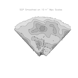
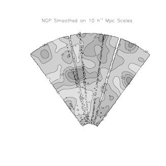
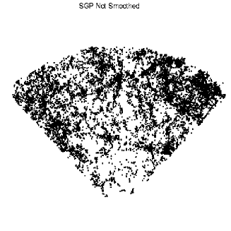
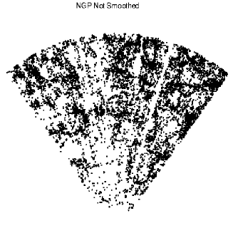
Figure 1: Smoothed and unsmoothed contour maps of the density of objects in the SGP and NGP slices. The darker the contour, the denser the region. In the smoothed plots, the darkest contours are 2$\sigma$ over-dense regions and the lightest contours are the 2$\sigma$ under-dense regions. The 2D smoothing kernel is a Gaussian with dispersion $\lambda=10h^{-1}$Mpc. Small differences in the qualitative appearance of the smoothed and unsmoothed maps are due to incompleteness of the survey. This incompleteness and the varying thickness of the slices with redshifts are accounted for in the smoothed maps.

In the NGP region we have 11375 galaxies and in the SGP region there are 12062 galaxies in our volume limited sample. The mean 3D galaxy-galaxy separation in the volume-limited samples is of order 7$h^{-1}$Mpc. This is then projected down into two dimensions, which reduces the mean 2D galaxy-galaxy separation. Therefore our choice of 10$h^{-1}$Mpc for the smoothing length in most of the genus calculations (see section 3) is large enough so that the genus signal is not dominated by Poisson shot noise.

2.1 The Simulation

To test the robustness of our statistical methods, estimate uncertainties in our measurement, and to test the currently best fitting variant of CDM, we use mock surveys drawn from the Virgo Consortium’s Hubble Volume $z=0$ $\Lambda$CDM simulation. This simulation contains 1 billion mass particles in a cube with side 3,000$h^{-1}$Mpc, large enough that many independent mock catalogs can be constructed. The cosmological parameters of the simulation are $\Omega_{\rm b}=0.04,\Omega_{\rm CDM}=0.26,\Omega_{\Lambda}=0.7,h=0.7,\Gamma=0.17$, close to the values suggested by median statistics analysis (Gott et al. 2001). The clustering amplitude of the dark matter particles closely matches that of present day, optically selected galaxies so no biasing has been applied. For more details see Frenk et al. (2000). This simulation does not include any gas physics but we generally smooth on large, 10$h^{-1}$Mpc, scales where the dark matter fluctuations might be expected to trace the clustering pattern of galaxies.

We construct samples that have the same geometry as the current 2dFGRS data using the same technique that we use to construct the random catalog. The only difference is that in the mock catalogs we sparsely sample the points to match the number density of galaxies in the 2dFGRS.

3 The Genus Statistic

The genus statistic is a quantitative measure of the topology of regions bounded by isodensity surfaces. In two-dimensions, that surface is simply the set of curves that separate high and low density areas. Here, we present results on the two-dimensional genus statistic (see Gott et al. 1986; Melott 1989; Melott et al. 1989; Gott et al. 1990; Park et al. 1992; Colley 1997). Following Melott et al., we define the 2-D genus to be

$$G_{2}={\rm number\;of\;isolated\;high\;density\;regions\;-\;number\;of\;isolated\;low\;density\;regions.}$$ (2)

The genus of a contour in a two-dimensional density distribution can also be calculated using the Gauss-Bonet theorem, in the two dimensional form, using

$$G_{2}=\frac{\int CdS}{2\pi}$$ (3)

where the line integral follows the contour and $C$ is the inverse curvature $r^{-1}$ of the line enclosing a high or low density region. This can be positive or negative depending on whether a high or low density region is enclosed. The genus of a contour enclosing an isolated high density region is positive, where as the genus of a contour enclosing a low density region is negative. This expression allows contributions from contours around regions that do not lie fully within the boundaries of the survey to be included.

For a Gaussian random field, the genus has a simple analytic form. The genus per unit area is expressed as

$$g_{2}=\frac{G_{2}}{\rm Area}=A\nu e^{-\nu^{2}/2},$$ (4)

where $\nu$ is the threshold value, above which a fraction, $f$, of the area has a higher density

$$f=(2\pi)^{-1/2}\int^{\infty}_{\nu}\exp(-x^{2}/2)dx$$ (5)

The value of the amplitude, $A$, depends on the shape of the power spectrum. Melott et al. (1989) describe the form that $A$ can take in extreme situations for varying power spectrum indices. i.e. if the smoothing length is much larger or smaller than the thickness of the slice. In our case the smoothing length is comparable to the thickness of the slice and the power spectrum index of the 2dFGRS is close to $n=-2$, thus neither of the approximations given in Melott et al. are appropriate here.

The steps to calculating the genus are as follows:

• Construct a random catalog of points for the NGP and SGP that have the same angular and radial selection function as the data points but with much higher number density

• Take the data points (the NGP and SGP points are considered separately) and the random points and place each of them on a grid. We have 256² cells in each grid. Calculate the density of data and random points in each cell.

• Smooth the data and random density field with a Gaussian kernel

• Divide the smoothed data density field by the smoothed random density field

• Mark the cells that lie outside the survey (i.e. the cells with density=0 in the unsmoothed random density field) with a negative value. These cells are then ignored by Contour2D

• Run CONTOUR2D

We smooth the data and random point density distributions by convolving the density field with a Gaussian of the form $e^{-r^{2}/(2\lambda)^{2}}$, where $\lambda$ is the smoothing scale, typically set here to 10$h^{-1}$Mpc. This value is chosen so that the structures that remain are in the quasi-linear regime. Note that this definition of the Gaussian smoothing length $\lambda$ differs from some earlier papers on the genus statistic (some earlier papers use $e^{-r^{2}/{\lambda}^{2}}$). The smoothed and unsmoothed NGP and SGP slices are shown in figure 1. Structures are clearly able to survive the small gaps in the currently incomplete data. The random points are used to mark the edge of the survey and to take out any contribution to the genus from the shape of the survey (c.f. the window function in power spectra analysis).

CONTOUR2D uses a two-dimensional variant of the angle deficit algorithm described by Gott et al. (1986). The density contour is specified by the fractional area contained in the high density region of the smoothed density field. The program classifies all cells as high or low density then evaluates the genus of the contour surface by summing the angle deficits at all vertices that lie on the boundary between the high and low density regions.

Figure 2: The genus of the NGP strip (open circles) and the SGP strip (filled circles) and the average genus (solid line). The points are offset slightly for clarity. A smoothing length of 10$h^{-1}$ Mpc was used in calculating the genus.

4 Results

In Figure 2, we present the genus of the 2dFGRS. We show the genus of the NGP (open circles) and the SGP (filled circles) as well as the average genus (solid line). The NGP and SGP genus curves have similar shapes, although the curves cross zero at different points. This is discussed in more detail in section 4.3. The amplitude of the SGP genus curve is also slightly higher than that of the NGP. In order to assess the significance of these results we compare the results to simulations and use a Mann-Whitney Rank Sum test to compare the data to the mock catalogs.

4.1 Simulations

To test the significance of the genus we measure from the 2dFGRS, we compare the results to a simulation, described in section 2.1. We extract 20 NGP and 20 SGP mock surveys from the $\Lambda$CDM Hubble Volume $z=0$ simulation.

We measure the genus of the 20 realizations of each slice and compute the average. We find that despite the different areas and thicknesses of the SGP and NGP regions the genus curves are very similar, shown in figure 3. The final SGP slice will be 5 degrees thicker than the NGP slice but currently the data cover similar declination ranges and thus similar genus curves are expected if the NGP and SGP data are large enough to cover representative regions of the universe. See Colless et al. (2001) for the masks of the public data release.

To test if the current geometry of the 2dFGRS significantly affects our estimate of the genus, we compare the genus derived from the mock catalogs to the genus found from simulation wedges that cover the full extent of the 2dFGRS (assuming the same averaged number density of points in the currently unobserved regions). Figure 4 shows the predicted final genus curve (solid line SGP, dashed line NGP) compared to the mock catalog genus curve for the NGP (open circles) and the SGP (filled circles). We see very little difference between the two NGP curves because the current NGP data covers most of the angle range of the expected final region. This shows that, despite the regions in the slice where there is no data, the genus curve can still be accurately recovered. In other words, the isolated peaks and holes in the density distribution are adequately sampled in the incomplete density distribution.

There is more difference between the simulated incomplete and complete SGP curves as the final slice will cover a region that is approximately 5 degrees thicker in declination than the current data. The thicker slice suppresses the number of isolated high and low density regions that can be detected because the data is effectively smoothed in the declination direction. This gives rise to a less than 1$\sigma$ difference in the curve, suggesting the genus curve presented here will be very similar to that from the final sample. If the complete data covers the full 15 degree declination range in the south, a scaling factor may be required if the genus of the NGP and SGP are to be averaged together or a 10 degree region could be extracted from the SGP region.

Data Source	Amplitude	Rank	Significance	Shift	Rank	Significance
2dFGRS NGP	8.2$\pm 1.2$	9	0.42 $<1\sigma$	-0.20$\pm-0.09$	6	0.28 $<1\sigma$
2dFGRS SGP	9.2$\pm 1.0$	15	0.71 $<1\sigma$	0.18$\pm-0.07$	18	0.86 $\sim 1\sigma$
2dFGRS Combined	8.8$\pm 0.85$	13	0.62 $<1\sigma$	-0.02$\pm-0.06$	12	0.57 $<1\sigma$

Table 1: The rank of the amplitude and shift for the NGP, SGP and average genus curves (smoothing length 10$h^{-1}$Mpc) as compared to the 20 realizations. The ranking gives the position of the data with respect to the 20 mock catalogs, i.e. a ranking of 9 means there are 8 mock catalogs with smaller values and 12 with larger values of the feature we are testing.

4.2 Error Analysis

We use the simulations as a method for estimating the errors on the genus curve measured from the 2dFGRS. The two-point clustering amplitude of the $\Lambda$CDM Hubble Volume simulation is close to that of present day, optically selected galaxies (see Hoyle et al. 1999). In figure 5, we compare the average simulation NGP and SGP genus curve with the curves measured from the 2dFGRS for two choices of the smoothing length. We find that the two curves have approximately the same shape and amplitude and therefore it seems reasonable to use the errors from the simulation as estimates for the errors in the data.

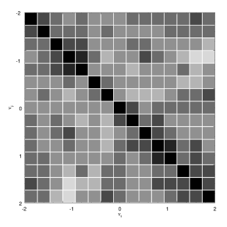
Figure 6: The normalized covariance matrix of genus estimates $G(\nu_{i})$. The diagonal elements show the variance. The off diagonal elements show the amount of correlation between different points. We normalize the covariance in each grid cell by $C^{\prime}_{i,j}=C_{i,j}/(\sqrt{C_{i,i}}\sqrt{C_{j,j}})$. The darkest shadings show where the covariance between points is the strongest. The lightest shadings show where points are strongly anti-correlated. Mid grey shadings show where there is no correlation (either positive or negative) between points. The values of $C^{\prime}_{i,j}$ shown by the different shadings are given in the legend above the covariance matrix.

The individual genus points are not independent, thus it is important to evaluate the full covariance matrix of the measurement. We average the mock NGP and SGP genus curves together to create mock average genus curves. From these, we calculate the covariance matrix. This is shown graphically in figure 6, where for clarity the value of the covariance in each bin has been normalized according to $C^{\prime}_{i,j}=C_{i,j}/\sqrt{(C_{i,i}C_{j,j})}$. The covariance matrix is strongest down the diagonal elements, as expected. Around the peaks of the genus curve, near $\nu=$ -1 and 1, there is strong covariance between neighboring points. This covariance makes physical sense; the maximum amplitude of the genus curve depends on the finite number of isolated clusters or voids that lie within the survey region. The peaks of the genus curve are anti-correlated with each other. This result might be explained by the anti-correlation between the physical locations of clusters and voids; a region of space with a few extra clusters is less likely to have an excess of large voids within it.

4.3 Amplitude and Shift of the Genus

To quantify departures away from the random phase genus curve, we can compute two statistics, termed Genus Meta-Statistics (see Vogeley et al. 1994 for an application in three dimensions). These are the amplitude of the genus curve and the shift of the genus curve (i.e. where the curve has a genus value of zero [a Gaussian random field has zero genus at the median density of $\nu=0$]). We use these two statistics to compare the measured genus curve with that of a Gaussian random field and an $\Lambda$CDM N-body simulation. The amplitude contains information about the slope of the power spectrum; the more power at large scales, the lower the amplitude of the genus curve. The amplitude of the genus curve also contains information about the non-linear clustering. A Gaussian random field that has not been allowed to evolve under gravity will have a higher genus amplitude than a field with the same power spectrum that has undergone non-linear evolution. We discuss this effect in more detail in below.

To measure the amplitude, we simply find the best fit Gaussian random phase curve (equation 4) to the data to minimize $\chi^{2}$. We could use the full covariance matrix in this calculation to prevent the result being biased by high or low points that are highly correlated. However, an accurate estimation of the covariance is hard to obtain as it depends on very high order moments of the galaxy density field. Even if the true clustering of galaxies is well described by the $\Lambda$CDM model, 20 mock surveys may be insufficient to accurately estimate the covariance.

Figure 3: The left hand plot compares the average genus of the $\Lambda$CDM mock NGP (open circles) and SGP (filled circles) catalogs and the genus found by averaging the NGP and SGP together (smoothing length 10$h^{-1}$Mpc). The points are slightly offset for clarity. The center and right hand plots show the NGP and SGP mock catalogs with the average genus shown by the dark line with error bars. 5 of the 20 independent realizations are shown in these figures to give an idea of the range of genus curves that can be obtained with the current 2dFGRS geometry.

Figure 4: A comparison of the genus from the mock NGP and SGP catalogs with the current incomplete geometry imprinted onto them (open points - NGP, filled points - SGP) to the NGP and SGP genus curves we predict for the completed regions (dashed lines - NGP, solid lines - SGP). All curves are for Gaussian smoothing length $\lambda=10h^{-1}$Mpc.

We fit the amplitude of the mock catalog genus curves to see how strongly the off-diagonal covariance matrix points affect the fitting of the amplitude. The amplitudes are slightly higher using only the diagonal elements as the points around the peaks are most strongly correlated, although we find that the amplitude of the fits to the simulations are consistent whether we only use the diagonal elements or the full covariance matrix. However, when we fit the 2dFGRS data, we find very different results with and without the off diagonal matrix elements. In the case of the NGP the best fit amplitude when we use the full covariance matrix is 4.2$\pm 1.1$ , which is clearly too low. This value is obtained due to points with negative $\nu$ which do not fit a Gaussian shape. When we use only the diagonal elements we find a value of 8.2$\pm 1.2$ for the NGP sample. Visually this looks consistent with the data. The SGP does not have the same problem; we find the result is 9.2$\pm 1.0$ using the diagonal elements only and 8.8$\pm 0.9$ using the full covariance matrix. We therefore just use the diagonal elements when fitting the amplitude of the data but we add a word of caution that these may be slightly high by $\sim 10\%$ due to the covariance between the points around the peaks of the genus curve. These values are given in table 1.

If the measured genus crosses zero at values less than zero then the data has a meatball topology, i.e. the isolated clusters are more emphasized then the low density regions, if the shift is to the right then the data has a bubble topology, i.e. there is an excess of isolated voids compared to the high density regions. Biased CDM models tend to display a more meatball like topology whereas hot dark matter models tend to have a bubble topology (Melott et al. 1989). We determine the zero point shift by simply looking at where the genus curves have zero value. This value can be read off the genus plots directly.

We compare the shift and amplitude values that we obtain from the 2dFGRS to the values that we estimate from the 20 mock catalogs. We perform a nonparametric, Mann-Whitney rank sum test to examine whether results from the data are consistent with the simulation. The rank of the various meta statistics as measured from the data is given in table 1. A rank of 8, for example, means there are 7 mock catalogs with smaller amplitude or lower zero point crossing than the data and thus 13 mock catalogs with larger values.

The NGP strip has a slightly lower amplitude than the SGP strip. The points near $\nu=-1$ have a lower amplitude in the NGP strip than in the SGP strip. This is probably the main source of the difference. The difference is around 1$\sigma$ only.

The NGP data also display a slight meatball topology whereas the SGP displays a bubble topology. On average, the difference is very small and consistent with the genus of a Gaussian random distribution.

We compare the $\chi^{2}$ values obtained when the data is fit by the best fit Gaussian curve and by the $\Lambda$CDM simulation. The curves are plotted in the right-most panel of figure 5. We find that the minimum $\chi^{2}$ value from the Gaussian curve is 25.5 where as the value of $\chi^{2}$ we obtain using the simulation is 30.2. We have 15 data points which suggests a $\chi^{2}$ per degree of freedom of order 2. However, the covariance matrix tells us that adjacent points are highly correlated, so this naive $\chi^{2}$ is not appropriate. Examination of the figure 5c shows that the fits are not that bad; the significant discrepancy near $\nu=+1$ is caused by three or four highly-correlated points that lie above the fitted curves. This departure suggests an excess of clusters in this data sample relative to a Gaussian distribution or the $\Lambda$CDM model but the excess is actually rather small when we consider the physical significance of this peak in the genus curve. Near $\nu=+1$ we measure the number of isolated clusters in the sample and obtain $G(1)\sim 7$. If the number of such structures within a region of this size obeys Poisson statistics, then this peak value has uncertainty of roughly $\pm\sqrt{7}$. Because peaks of a Gaussian random field are positively correlated, the fluctuations of the number of isolated clusters might be larger and the statistical significance of the apparent excess of clusters in the 2dFGRS may be quite smaller than the naive $\chi^{2}$ analysis suggests.

To examine whether the amplitude and shifts are dependent on the choice of the smoothing length, we also compute the genus curves for the 2dFGRS data using a smoothing of 5$h^{-1}$Mpc, using the identical volume-limited sample of the 2dFGRS. Note that 5$h^{-1}$Mpc is the smallest smoothing length for which both the correlation length of galaxies and the average galaxy-galaxy separation are smaller or comparable to the smoothing length. The genus curves for $\lambda=5h^{-1}$Mpc are shown in figure 7. We find again that the NGP curve has a slight meatball shift, whereas the SGP displays a slight bubble shift. There is better agreement between the amplitudes of the two curves than for $\lambda=10h^{-1}$Mpc, although in the 10$h^{-1}$Mpc case any difference between the amplitudes was less than 1$\sigma$. The difference between the genus curve of the data and the $\Lambda$CDM simulation using the smaller smoothing length is slightly larger. This difference is because we are probing smaller scales at which the clustering of the $\Lambda$CDM simulation does not match the clustering of present day, optically selected galaxies as well (see, for example, Hoyle et al. 1999). We compare the genus curve to a random phase curve, where the amplitude has been selected to minimize $\chi^{2}$. Again, we find that there is an excess of clusters over voids in the 2dFGRS data. Therefore we conclude that the results we present above are not dependent on the choice of the smoothing length.

Figure 5: A comparison of the measured 2dF genus compared to the mock catalog $\Lambda$CDM simulation genus curve (smoothing length 10$h^{-1}$Mpc). On the left we show the results for the NGP. In the center we show the results for the SGP. On the right, we compare the average genus of the 2dFGRS with the genus of the $\Lambda$CDM simulation (dashed line) and a best fit random phase curve (solid line) where the amplitude has been chosen to minimize $\chi^{2}$.

Figure 7: A comparison of the measured 2dFGRS genus compared to the mock catalog $\Lambda$CDM simulation genus curve calculated using a smoothing length of 5$h^{-1}$Mpc. On the left we show the results for the NGP, the SGP and the average genus curve of the 2dFGRS. On the right, we compare the average genus of the 2dFGRS calculated using a smoothing length of 5$h^{-1}$Mpc with the genus of the $\Lambda$CDM simulation (dashed line) and a best fit random phase curve (solid line) where the amplitude has been chosen to minimize $\chi^{2}$.

Figure 8: The 2dFGRS genus curve (smoothing length 10$h^{-1}$Mpc) compared to a genus curve taken from 10 realizations of a Gaussian Random Field with the power spectrum matching that of the 2dFGRS. We detect an excess of isolated clusters in the 2dFGRS genus curve.

4.4 Gaussian Random Field Comparison

As a final comparison, we compare the genus of the 2dFGRS with the genus of a Gaussian Random Field (GRF) that has the same power spectrum as the 2dFGRS. The power spectrum of the 2dFGRS has been measured by Percival et al. (2001) but is only presented in a form where it is divided by a linear theory power spectrum with values of $\Omega_{\rm m}h=0.2,\Omega_{\rm b}/\Omega_{\rm m}=0$ with $n$=1 and $\sigma_{8}$=1. We use CMBFAST to construct such a power spectrum, assuming that $h$=0.7 and that $\Omega=\Omega_{\rm m}+\Omega_{\Lambda}$=1. We multiply the points presented in Percival et al. to obtain an estimate of the 2dFGRS power spectrum. We also measure the power spectrum from the two NGP and SGP volume-limited samples we have constructed here to check consistency and find that the three power spectra have approximately the same shape. On scales larger than 10$h^{-1}$Mpc and up to 400$h^{-1}$Mpc, the 2dFGRS P(k) is fairly similar in shape to the CMBFAST power spectrum. To test how sensitive the genus curve is to the exact features in the power spectrum curve, we compare the genus curves we obtain using a power law with P$\propto k^{-2}$, the CMBFAST power spectrum and the estimate of the 2dFGRS power spectrum we obtain here and find little difference between the CMBFAST and 2dFGRS genus curves and only small differences between these genus estimates and ones created with the power law input. We construct the GRF on a 256³ array by assigning values to the real and imaginary parts of each Fourier mode which are Gaussian deviates. We then imprint the shape of the NGP and SGP regions onto the grid before we smooth the density field and calculate the genus, exactly as described above.

We compare the genus of the 2dFGRS with that of a GRF with the same power spectrum to see if the non-linear clustering that appears in the data and in the simulations affects the amplitude of the 2D genus. In previous papers that examine the genus in 3D, significant damping of the amplitude of the data genus curve has been found as compared to the genus curve of a GRF. Vogeley et al. (1994) found that for smoothing scales of 6$h^{-1}$Mpc that a GRF had a 2$\sigma$ higher amplitude than the genus curve of the CfA survey. On larger smoothing scales this difference was reduced and at 16$h^{-1}$Mpc, the two curves had consistent amplitude.

We find in 2D that we do not see the same damping that has previously been seen in the 3D genus. For values of $\nu<0$, the amplitude of the GRF genus curve is fairly similar to that of the 2dFGRS but on positive $\nu$ scales, the amplitude is lower than the 2dFGRS. On these large scales, the data is definitely showing an excess of overdensities, as shown earlier in figure 5. The best fitting Gaussian curve has a comparable amplitude to the underdense part of the genus curve but a lower amplitude than the overdense part of the genus curve.

Several factors could account for the apparent discrepancy between the 2 and 3D genus amplitude ratios. It may be that our smoothing length of 10$h^{-1}$ is close enough to the linear regime that no amplitude difference due to non-linear clustering may be seen. Note that our 10$h^{-1}$Mpc smoothing length would be $\lambda=14.14h^{-1}$Mpc if we used the smoothing length definition adopted in in older genus papers. Vogeley et al. (1994) found no effect in 3D for $\lambda=16h^{-1}$Mpc. It may also be that the non-linear clustering has a smaller effect on the 2D genus, where data are projected and thereby smoothed over the width of the survey, thus making the effective smoothing length larger. However, we repeated this analysis using a 2D smoothing length of only 5$h^{-1}$Mpc and found similar results. Because an excess of clusters may reflect biasing of the galaxies with respect to the mass distribution, it will be interesting to repeat this analysis with the final data set to examine whether the completed sample exhibits this amplitude excess in the genus curve at high density thresholds. If these partial data in the 2dFGRS strips were slightly biased toward high density regions, perhaps because denser fields were given targeting priority over lower density regions during early observations, then the complete sample might lack such a feature.

5 Conclusions

We measure the genus from a 100,000 galaxy redshift sample of the 2dFGRS, the largest redshift sample publicly available to date. We find that the genus curves of the NGP and SGP are slightly different, with the NGP region displaying an excess of isolated clusters and the SGP region displays a slight excess of isolated voids. These shifts are only significant at the 1$\sigma$ level when we compare the genus curves to mock catalogs drawn from a $\Lambda$CDM simulation. The results are qualitatively the same for two choices of the smoothing length. We average the NGP and SGP data and find that the average genus curve is consistent with the $\Lambda$CDM simulation. We find that the average 2dFGRS genus curve reveals a smaller number of isolated voids than clusters in the Survey, although the points in the genus curve that show this slight excess of clusters are highly correlated.

We demonstrate that in spite of the current incompleteness in the geometry, the genus can be accurately recovered. No bias is introduced into the shape of the genus curve by the current angular coverage.

We compare the 2dFGRS genus curve with that for a GRF with the same power spectrum. We do not find any significant amplitude depression in the amplitude of the 2dFGRS genus curve due to non-linear clustering. This may be due to the large smoothing length, may be a feature of the 2D genus, or may indicate a real excess in the number of isolated clusters in the the 2dFGRS that is not predicted directly from the power spectrum alone. Colley (1997) found that the 2D genus of the Las Campanas Redshift Survey agrees well with a Gaussian random field. A larger sample of galaxies will reveal whether there really is an excess of over dense regions, or whether this is a feature of the observing strategy applied so far.

References

- (1) Bardeen, J. M., Steinhardt, P. J., & Turner, M. S., 1983, Phys. Rev., 28, 679
- (2) Bahcall, N. A., Ostriker, J. P., Perlmutter, S. & Steinhardt, P. J, 1999, Science, 284, 1481
- (3) Canavezes, A., et al., 1998, MNRAS, 297, 777
- (4) Colless, M., et al., 2001, MNRAS submitted, astro-ph/0106498
- (5) Colley, W. N., 1997, ApJ, 489, 471
- (6) Colley, W. N., Gott, J. R. III, & Park, C., 1996, MNRAS, 281, L2
- (7) Frenk C.S.. et al., 2000, astro-ph/0007362
- (8) Gott, J.R. III, Vogeley, M.S., Podariu, S., & Ratra, B. 2001, ApJ, 549, 1
- (9) Gott, J. R. III, Melott, A. L., & Dickinson, M., 1986, ApJ, 306, 341
- (10) Gott, J. R. III, et al., 1989, ApJ, 340, 625
- (11) Hoyle F., Baugh C. M., Shanks T. & Ratcliffe A., 1999, MNRAS, 309, 659
- (12) Maddox, S. J., Efstathiou, G., Sutherland, W. J., & Loveday, J., 1990a, MNRAS, 243, 692
- (13) Maddox, S. J., Efstathiou, G., & Sutherland, W. J. 1990b, MNRAS, 246, 433
- (14) Melott, A. L., 1989, Physics Reports, 193, 1
- (15) Melott, A. L., Cohen, A. P., Hamilton, A., Gott, J. R. III, & Weinberg, D., 1989, ApJ, 345, 618
- (16) Norberg, P. et al., 2001, MNRAS submitted, astro-ph/0105500
- (17) Park, C., Gott, J. R. III, da Costa, L. N., 1992, ApJ, 392, L51
- (18) Park, C., Gott, J. R. III, Melott, A. L., & Karachentsev, I. D., 1992, ApJ, 387, 1
- (19) Percival, W. J., et al., 2001, MNRAS, submitted, astro-ph/astro-ph/0105252
- (20) Vogeley, M.S., Park, C., Geller, M. J., Huchra, J.P., & Gott, J.R. III, 1994, 420, 545
- (21) Zucca, E., et al., 1997, A&A, 326, 477