Neutrinos from active galactic nuclei as a diagnostic tool

Active galactic nuclei (AGN) are known as sources of high energy $\gamma$-rays. The emission probably results from non-thermal radiation of relativistic jets belonging to the AGN. Earlier investigations of these processes have suggested that neutrinos are among the radiation products of the jets and may be used to discriminate between hadrons and leptons as primary particles for the production of the high energy emission. Our calculation of the high energy neutrino emission from the jets of AGN is based on a recently published model for $\gamma$-ray production by a collimated, relativistic blast wave, in which the spectral evolution of energetic particles is determined by the interplay between the particle injection by sweep-up of the interstellar medium, the energy losses through radiation, and diffusive escape. It is important to note that the swept-up interstellar particles retain their relative velocities with respect to the jet plasma, but get isotropised in the jet rest frame by self-excited $\rm Alfv\acute{e}nic$ turbulence. The bulk of the neutrino emission is expected in the energy range between 100 GeV and a few TeV. It is shown that the neutrino flux is correlated with the flux of TeV $\gamma$-rays. This allows to distinctly search for neutrino emissions from the jets of AGN by using the TeV $\gamma$-ray light curves to drastically reduce the temporal and spatial parameter space. Given the observed TeV photon fluxes from nearby BL Lacs the neutrino signal from AGN may be detectable with future neutrino observatories as least as sensitive as IceCube.

1 Introduction

To date, more than 60 blazar-type active galactic nuclei (AGN) have been detected as emitters of MeV-GeV $\gamma$-rays by EGRET (von Montigny et al. cvm95 (1995), Mukherjee et al. muk97 (1997)), and another few BL Lacertae objects have been observed as sources of TeV $\gamma$-rays by ground-based Čerenkov telescopes (Catanese & Weekes cw99 (1999)). In these sources the bulk of luminosity is often emitted in the form of $\gamma$-rays. The $\gamma$-ray emission of the typical blazar is highly variable on all timescales down to the observational limits of days at GeV energies and hours at TeV energies (e.g. Mattox et al. mat97 (1997), Gaidos et al. gai96 (1996)). Emission constraints such as the compactness limit and the Elliot-Shapiro relation (Elliot & Shapiro es74 (1974)) are violated in some $\gamma$-ray blazars, even when these limits are calculated in the Klein-Nishina limit (Pohl et al. poh95 (1995), Dermer & Gehrels dg95 (1995)), which implies relativistic bulk motion within the sources. This conclusion is further supported by observations of apparent superluminal motion in many $\gamma$-ray blazars (e.g. Pohl et al. poh95 (1995), Barthel et al. bar95 (1995), Piner & Kingham 1997a ; 1997b ).

Most published models for the $\gamma$-ray emission of blazars are based on inverse Compton scattering of soft target photons by highly relativistic electrons in the jets of these sources. The target photons may come directly from an accretion disk (Dermer et al. dsm92 (1992), Dermer & Schlickeiser ds93 (1993)), or may be rescattered accretions disk emission (Sikora et al. sbr94 (1994)), or may be produced in the jet itself via synchrotron radiation (e.g. Bloom & Marscher bm93 (1996) and references therein). The criticism of these models focuses on the fact that an electron acceleration process would have to be very fast to compete efficiently with the radiative losses at high electron energies, and it is therefore unlikely that the electrons are the primary particles.

The radiating electrons can also be secondary particles produced in inelastic collisions by primary hadrons, in which case neutrinos would be emitted in parallel to the $\gamma$-rays. Neutrinos can therefore be used to distinguish between purely leptonic models and models which involve high energy hadrons as primary particles.

One class of hadronic models is based on proton acceleration to ultra high energies around $10^{20}\$eV, so that photomeson production on ambient target photons can provide many secondary electrons and positrons (Kazanas & Ellison ke86 (1986), Sikora et al. sik87 (1987), Mannheim & Biermann mb92 (1992)). Such systems are usually optically thick and a pair cascade develops. These models are particularly attractive because they allow a possible link be made between escaping ultra high energy hadrons and the cosmic ray spectrum at $10^{20}\$eV near earth (e.g. Waxman wax95 (1995)). Steady-state calculations indicate that blazars would produce a high flux of neutrinos with energies up to $10^{19}\$eV (Mannheim man95 (1995), Halzen & Zas hz97 (1997), Protheroe pro97 (1997)). Note, however, that some of these results appear to be in conflict with physical upper limits for the total neutrino intensity produced by ultra high energy hadrons in AGN (Waxman & Bahcall wb99 (1999), Bahcall & Waxman bw01 (2001)). It is unfortunate that time-dependent calculations of proton-induced cascades have never been performed. We can therefore not comment on possible correlations between the neutrino flux of a source and its variable GeV-TeV $\gamma$-ray emission, for the latter is also influenced by the presumably variable pair-pair optical depth.

Two of us have recently published a new model of particle energization in jets of AGN, which is motivated by the blast wave models of gamma-ray bursts (Pohl & Schlickeiser ps00 (2000)). There the AGN jet is assumed to be a cloud of dense plasma which moves relativistically through the interstellar medium of the AGN host galaxy. It was shown that swept-up ambient matter is quickly isotropised in the blast wave frame by a relativistic two-stream instability, which provides relativistic particles in the jet without invoking any acceleration process. The typical primary particle would be a proton with a Lorentz factor of the order of one hundred, distributed isotropically in a jet which also moves with a bulk Lorentz factor of the order of one hundred. Inelastic proton-proton collisions with the background plasma would then lead to the production of TeV $\gamma$-rays by $\pi^{0}$-decay as well as synchrotron, inverse Compton, and bremsstrahlung emission produced by secondary electrons at lower energies. The fully time-dependent calculations show that the observed variability behavior and $\gamma$-ray spectra of blazars can be explained with this model.

In this paper we are concerned with the neutrino emission which is produced in parallel to the $\gamma$-rays during the decay of the charged pions. We shall provide specific predictions for the neutrino flux and spectra in relation to the TeV $\gamma$-ray emission of AGN. These will allow observers to a) search for neutrino emission of AGN by using the TeV $\gamma$-ray light curves as indicator of activity, and b) perform a decisive test of at least one hadronic model of $\gamma$-ray production in AGN.

In Sect. 2 we briefly review the spectral evolution of the energetic protons, resulting from the interplay between the injection and the losses. We discuss some resulting proton spectra and show that the spectral evolution of the proton distribution depends on the geometry and the physical constitution of the blast wave. In Sect. 3 we discuss the various decay modes and present the the source functions for the decay processes of the charged pions as well as the subsequent decay of charged muons.

We also investigate the emission of electron anti-neutrinos caused by $\beta$-decay of neutrons produced in $p+p\rightarrow p+n+X$ reactions. We show that the power radiated in thus produced $\overline{\nu}_{e}$ emission is about two orders of magnitude smaller than the power radiated in the form of electron (anti-)neutrinos arising from the decay of muons. In Sect. 4 we discuss the spectral evolution of the neutrino emission, induced by the proton spectra presented in Sect.2. We show that (muon)-neutrino emission at energies around 1 TeV is correlated with TeV $\gamma$-emission.

2 The energy distribution of protons in an AGN jet

The AGN model of Pohl & Schlickeiser (ps00 (2000)) describes the jet as a plasma could consisting of electrons and protons, that is assumed to have a cylindrical shape with thickness $\rm{d}$, where $\rm{d}$ is small compared to the radius $\rm{R}$ (see also Fig.1). The jet is moving with a bulk Lorentz factor $\Gamma$ through the ambient medium. Viewed in the rest frame of the jet plasma cloud, the interstellar medium forms an electron-proton beam of density $n_{\rm i}=\Gamma\,n_{\rm i}^{*}$, which is small compared with the plasma density $n_{\rm b}$ of the jet cloud. Using kinetic theory Pohl & Schlickeiser (ps00 (2000)) have shown, that the incoming particles of the interstellar medium quickly get isotropised by self-excited $\rm Alfv\acute{e}nic$ turbulence, but retain their relative velocities with respect to the jet plasma. The jet plasma thus becomes enriched with relativistic particles, of which only the protons are of interest for us, for they can produce neutrinos.

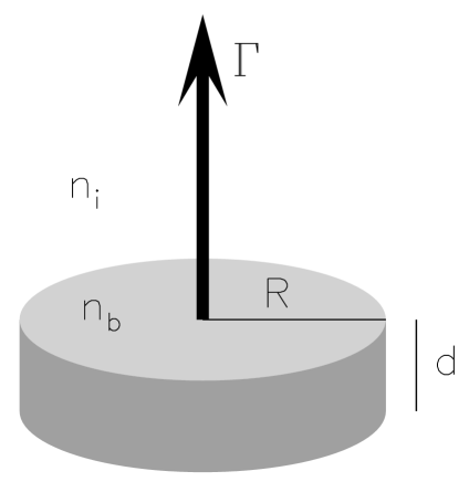
Figure 1: Sketch of the basic geometry. The thickness of the channeled blast wave $d$, measured in its rest frame, is much smaller than its halfdiameter. The blast wave moves with a bulk Lorentz factor $\Gamma$ through ambient matter of density $n_{\rm i}$.

Figure 2: A typical spectral evolution for protons in the blast wave, responsible for the neutrino emission. In this example the following parameters have been used: The radius of the plasma disk is $R=10^{14}\,\rm{cm}$,  the thickness of the disk amounts to $d=3\cdot 10^{13}\,\rm{cm}$  and the initial Lorentz factor is $\Gamma_{0}=300$.  The constant densities inside and outside the jet are $n_{b}=5\cdot 10^{8}\,\rm{cm^{-3}}$ and $n_{i}^{\ast}=0.2\,\rm{cm^{-3}}$, respectively. Note that the mentioned time refers to the observer frame and therefore depends on the viewing angle $\theta$, which we choose to be $0.1^{\circ}$ in this example.

This has two consequences:

a) the system is not stationary. For reasons of momentum conservation the Lorenz factor $\Gamma$ decreases at a rate

$$\dot{\Gamma}=-\frac{\pi\,R^{2}\,n_{i}^{*}\,c\,m_{p}}{M(t)}(\Gamma^{2}-1)^{3/2}.$$ (1)

Note that the relativistic mass

$$M(t)=\int_{1}^{\infty}\gamma\ m_{p}N(\gamma,t)\ d\gamma$$ (2)

is obtained from the particle spectrum in the jet plasma

$$N(\gamma,t)=V\,(n(\gamma,t)+n_{b}\,\delta(\gamma-1-\epsilon)).$$ (3)

in which, in contrast to the nomenclature used in Pohl and Schlickeiser (ps00 (2000)), we have have included the background plasma with a formal thermal energy $\epsilon=\frac{k\,T}{m_{p}\,c^{2}}\ll 1.$

b) relativistic protons are injected in the jet plasma at a rate

$$S(\gamma,t)=\pi R^{2}n_{i}^{*}c\sqrt{\Gamma(t)^{2}-1}\,\delta(\gamma-\Gamma(t))$$ (4)

where $\Gamma(t)$ is determined by Eq. 1. The temporal evolution of the proton spectra $N(\gamma,t)$ can be described by the continuity equation:

$$\frac{\partial N(\gamma,t)}{\partial t}+\frac{\partial(\dot{\gamma}N(\gamma,t))}{\partial\gamma}+\frac{N(\gamma,t)}{T_{E}}+\frac{N(\gamma,t)}{T_{N}}=S(\gamma,t)$$ (5)

We consider continuous energy losses from elastic and inelastic scattering at a rate of

$$-\dot{\gamma}=3\cdot 10^{-16}n_{b}\frac{\gamma}{\sqrt{\gamma^{2}-1}}+7\cdot 10^{-16}n_{b}\frac{(\gamma-1)^{2}}{\gamma+1}.$$ (6)

Additionally, one has to consider catastrophic particle losses arising from diffusive escape at the timescale of

$$T_{E}=\frac{3\,d^{2}}{\lambda\,\beta\,c}\,\simeq 1.67\,10^{-19}\,\frac{d^{2}\,\Gamma\,n_{i}^{\ast}}{\beta\,\sqrt{n_{b}}}\;\;\rm{s},$$ (7)

where $\lambda$ is the scattering length and $\beta=\sqrt{1-\gamma^{-2}}$.

Neutrons produced in $p\rightarrow n$ reactions are likely to escape the jet at a timescale of $T_{N}\simeq 3\cdot 10^{15}\,n_{b}^{-1}\;\rm{s}$ for $\gamma\gg 1$ (cf. Pohl and Schlickeiser ps00 (2000)).

Neglecting energy losses and additional particle losses, the continuity equation (5) becomes solvable and we get a $(\gamma^{2}-1)^{-3/2}$ spectrum for the particle distribution function $N(\gamma,t)$. However, more realistic cases require the use of numerical methods.

We use Eq. (1) to obtain the time $\tau^{\ast}$ at which the blast wave would be observed with a particular Lorentzfaktor $\Gamma$.

$$\tau^{\ast}=-\int_{\Gamma_{0}}^{\Gamma}\,d\Gamma^{\prime}\,\frac{\mathrm{M}(\Gamma^{\prime})\,}{C\,({\Gamma^{\prime}}^{2}-1)^{(3/2)}}\,\Gamma^{\prime}(1-\beta\cos\theta^{\ast})\,,$$ (8)

where $C=\pi\,R^{2}\,n_{i}^{\ast}\,c\,{m_{p}}$ and $\beta=\sqrt{1-\Gamma^{-2}}$. For the purpose of transformation to an observer frame one should bear in mind that the energy scales as well with the factor $\Gamma(1-\beta\cos\theta^{\ast})^{-1}$.

Figure 3: The proton spectra calculated with another set of parameters. Here we use $R=2\cdot 10^{15}\,\rm{cm}$ for the radius of the plasma disk and $d=10^{14}\,\rm{cm}$  for the thickness of the disk. The initial Lorentz factor stays at $\Gamma_{0}=300$.  The density in the jet has changed to $n_{b}=10^{8}\,\rm{cm^{-3}}$ and for the density outside the blast wave $n_{i}^{\ast}=1.5\,\rm{cm^{-3}}$ is assumed. Here the specified time refers to an viewing angle of $\theta=2^{\circ}$. In the bottom row the same spectra as in the top row are shown but with higher resolution.

In Fig. 2 and 3 we calculate typical examples of resulting proton distributions $N(\gamma,t)$, describing the number density of protons in terms of the Lorentz factor $\gamma$ w.r.t. the blast frame. Starting with an initial Lorentz factor of $\Gamma_{0}=300$ we show the distribution of protons for several instances of observed time corresponding to the reduced bulk Lorentz factors of the blast wave. According to Eq. 1 the Lorentz factor is monotonically decreasing. In all cases the sweep-up occurs at the present Lorentz factor in accordance with Eq. 4.

As mentioned before, the overall behaviour of the particle spectra is mainly determined by the competing modes of sweep-up and cooling of the particles. In Fig. 2 the swept-up particles cool down faster than the blast wave decelerates, whereas in Fig. 3, down to a Lorentz factor of $\Gamma=85$ the cooling is slow compared with the deceleration of the blast wave. Afterwards the deceleration rate of the blast wave is overtaken by the cooling rate of the particles. Then the competing mode of particle cooling is the more effective process. Determined by the initial parameters $d,R,n_{i}\ast$ and $n_{b}$ the spectra show a very different behavior. The time specified in the pictures refers to the observer frame and therefore depends on the viewing angle $\theta$.

3 The production of high energetic neutrinos

The energetic protons in the jet plasma produce pions in inelastic collisions with particles in the background plasma. For the calculation of the pion source spectra we use the Monte–Carlo model DTUNUC (V2.2) (Möhring & Ranft Moehring (1991), Ranft et al. Ranft (1994), Ferrari et al. 1996a , Engel et al. Engel (1997)), which is based on a dual parton model (Capella et al. Capella (1994)). Here we are concerned with high energetic neutrinos resulting from the decays of pions $\pi^{\pm}\rightarrow\mu^{\pm}+\,\nu_{\mu}(\overline{\nu}_{\mu})$ and subsequently $\mu^{\pm}\rightarrow e^{\pm}+\,\overline{\nu}_{\mu}(\nu_{\mu})+\,\nu_{e}(\overline{\nu}_{e})$.

3.1 Pion decay

Figure 4: The production rate of muon neutrinos resulting from the various decay modes calculated for one proton of kinetic energy $10\;\rm{GeV}$ and $100\;\rm{GeV}$, respectively. The emission rate does not change in the energy regime of a proton up to a range of $100\;\rm{GeV}$. Additionally we show the emission of $\gamma$-rays resulting from the decay $\pi^{0}\rightarrow 2\gamma$ displayed with the solid line. The emission from the positively charged pions and muons is slightly higher than the emission from the negative ones. The respective pion decay is more effective.

Figure 5: For a proton with the same kinetic energy as above the electron neutrino emission is shown here. The production of $\overline{\nu}_{e}$ and $\nu_{e}$ resulting from the muon decay is displayed by the solid line. The energy of anti-electron neutrinos produced by $\beta$-decay is about 2 orders of magnitude smaller. The complete rates of muon neutrinos and $\gamma$-rays are also depicted for reference.

The pion decay muon neutrino source function  $Q_{\nu}^{\pi}(E_{\nu},t)$ describing the energy spectrum of the neutrinos produced in the jet via pion decay can be written as

$$Q_{\nu}^{\pi}(E_{\nu},t)=\int\limits_{\gamma_{\pi\,min}}^{\infty}\,f(\gamma_{\pi})\,q_{\pi}(\gamma_{\pi},t)\;\;d\gamma_{\pi},$$ (9)

where $Q_{\pi}$ is the pion source function and

$$f(\gamma_{\pi})=\frac{1}{2\,{E_{\nu}^{0}}\,\sqrt{{\gamma_{\pi}}^{2}-1}}\,$$ (10)

is the normalized neutrino spectrum describing the two-body decay in the rest frame of the plasma (Stecker Stecker (1971), Marscher et al. Marscher (1980)). Here $E_{\nu}^{0}\simeq 29.79\;\rm{MeV}$ denotes the energy of the emitted neutrino in the CMS. The lower limit of integration is given by

$$\gamma_{\pi\,min}=\frac{E_{\nu}^{0}}{2\,{E_{\nu}}}+\frac{E_{\nu}}{2\,{E_{\nu}^{0}}}.$$ (11)

The pion source function giving the amount of pions per $\rm{cm^{3},\;GeV\;and\;s}$ can be calculated as an integral over the spectrum of energetic protons and the differential pion production cross section which we derive using the Monte–Carlo code DTUNUC.

$$q_{\pi}(\gamma_{\pi},t)=\int\limits_{1}^{\infty}n_{b}\,N(\gamma_{p},t)\,\beta\,c\,\frac{d\,\sigma(\gamma_{p})}{d\,\gamma_{\pi}}\;d\gamma_{p}\;\;\;$$ (12)

Here $\beta=v_{p}/c$ denotes velocity of the protons. It is convenient to perform the integration over the pion Lorentz factor in Eq. 9 first. Hence

$$Q_{\nu}^{\pi}(E_{\nu},t)=\int\limits_{1}^{\infty}n_{b}\,\beta\,c\,N(\gamma_{p},t)\!\!\!\!\!\!\int\limits_{\gamma_{\pi\,min}}^{\infty}\!\!\!\!\!f(\gamma_{\pi})\,\frac{d\,\sigma(\gamma_{p})}{d\,\gamma_{\pi}}d\gamma_{\pi}\;d\gamma_{p}\;\;\;$$ (13)

is the differential production rate of particles per $\rm{cm^{3}}$, GeV and s.

3.2 The neutrino production via decay of charged muons

In the decay of the pions charged muons emerge producing neutrinos in a second decay $\mu^{\pm}\rightarrow e^{\pm}+\,\overline{\nu}_{\mu}(\nu_{\mu})+\,\nu_{e}(\overline{\nu}_{e})$. The muon decay source functions for muon and electron neutrinos $Q_{\nu}^{\mu}(E_{\nu},t)$ are:

$$Q_{\nu}^{\mu}(E_{\nu},t)=\frac{1}{2}\!\!\!{\int\limits_{\gamma_{\mu,\,min}}^{\infty}\!\!\!\!f(E_{\nu})\!\!\int\limits_{\chi_{min}}^{1}\!\!q_{\pi}(\gamma_{\pi},t)\;{\frac{\partial{\gamma_{\pi}}}{\partial{\gamma_{\mu}}}}\,d\chi d\gamma_{\mu}}$$ (14)

with the neutrino spectrum $f(E_{\nu},\gamma_{\mu})$ in the rest frame of the plasma describing the three-body muon decay (Marscher et al. Marscher (1980), Zatsepin & Kuz’min Zatsepin (1962)): $\displaystyle f(E_{\nu})=16\,{\gamma_{\mu}}^{5}\,(\,\frac{3}{{\gamma_{\mu}}^{2}}-\frac{4}{3}(3+{\beta_{\mu}}^{2})\,\zeta\,)\,\zeta^{2}\,\frac{1}{m_{\mu}\;c^{2}}$

for

$$0\,\leq\,\zeta\,\leq\,\frac{1-\beta_{\mu}}{2}$$ (15)

and

$$f(E_{\nu})=\frac{(\frac{5}{3}+\frac{4}{(1+{\beta_{\mu}})^{3}}(\frac{8\,\zeta}{3}-3(1+{\beta_{\mu}}))\,\zeta^{2}\,)}{{\beta_{\mu}}\,\,{\gamma_{\mu}\;m_{\mu}\;c^{2}}}$$

for

$$\frac{1-\beta_{\mu}}{2}\,\leq\,\zeta\,\leq\,\frac{1+\beta_{\mu}}{2}\;$$ (16)

for muon neutrinos $\nu_{\mu}$ and electron neutrinos $\nu_{e}$. The spectra for the production of anti-muon neutrinos $\overline{\nu}_{\mu}$ and anti-electron neutrinos $\overline{\nu}_{e}$ are calculated by:

$$f(E_{\nu})=32\,{\gamma_{\mu}}^{5}\,(\,\frac{3}{{\gamma_{\mu}}^{2}}-2(3+{\beta_{\mu}}^{2})\,\zeta\,)\,\zeta^{2}\,\frac{1}{{m_{\mu}\;c^{2}}}$$

for

$$0\,\leq\,\zeta\,\leq\,\frac{1-\beta_{\mu}}{2}$$ (17)

and

$$f(E_{\nu})=\frac{(1+\frac{4}{(1+{\beta_{\mu}})^{3}}(4\,\zeta-3(1+{\beta_{\mu}}))\,\zeta^{2}\,)}{{2\beta_{\mu}}\,{\gamma_{\mu}\;m_{\mu}\;c^{2}}}$$

for

$$\frac{1-\beta_{\mu}}{2}\,\leq\,\zeta\,\leq\,\frac{1+\beta_{\mu}}{2}\;$$ (18)

where $\zeta=(\frac{E_{\nu}}{\gamma_{\mu}\,m_{\mu}\,c^{2}})$ and $\beta_{\mu}=v_{\mu}/c.$ Here $\gamma_{\pi}(\gamma_{\mu},\chi)$ denotes the Lorentz factor of the parent pion:

$${\gamma_{\pi}}=\frac{{\varepsilon_{2}}\,{\varepsilon_{1}}+\chi\,\sqrt{{\varepsilon_{2}}^{2}-{\varepsilon_{1}}^{2}+\chi^{2}}}{{\varepsilon_{1}}^{2}-\chi^{2}},$$ (19)

where ${\varepsilon_{1}}=3.68$,   ${\varepsilon_{2}}=3.55\,\gamma_{\mu}$ and $\chi$ is the CMS interaction angle cosine.

The lower limits of integration of (14) are:

$$\gamma_{\mu,\;min}=\frac{E_{\nu}\,}{m_{\mu}\,c^{2}}+\,\frac{m_{\mu}\,c^{2}}{4\,E_{\nu}}$$ (20)

and

$$\chi_{min}=\left\{\begin{array}[]{c@{\quad:\quad}l}-1&{\varepsilon_{1}}\leq{\varepsilon_{2}}\\ \sqrt{{\varepsilon_{1}}^{2}-{\varepsilon_{2}}^{2}}&{\varepsilon_{1}}>{\varepsilon_{2}}\end{array}\right.$$

The calculation of the source function $Q_{\pi}(\gamma_{\pi}(\gamma_{\mu},\chi),t)$ is based on the Monte Carlo code DTUNUC again and is calculated analogous to the previous case with formula 12.

Figure 6: The evolution of the muon neutrino emission resulting from the proton spectra of Fig. 2. The viewing angle is $\theta=0.1^{\circ}$ and the redshift of the AGN is $z=0.5$. All the other parameters are chosen as in Fig. 2. In the top row we see the $F_{\nu}$ spectra and in the bottom row the $\nu\,F_{\nu}$ spectra. The spectral evolution of the $\gamma$-ray production spectra is also shown for reference.

3.3 Neutron $\beta$-decay

The emission of electron anti-neutrinos resulting from the $\beta$-decay of secondary neutrons $n\rightarrow p+e+\overline{\nu}_{e}$ is described by the electron $\beta$-decay source function $Q_{\overline{\nu}_{e}}(E_{\nu},t)$ calculated analogous to Jones (Jones (1963)) treating the neutrino as a particle without mass:

$$Q_{\overline{\nu}_{e}}=\frac{1}{2}\int\limits_{0}^{Q}\!\frac{f(E_{\nu}^{0})}{E_{\nu}^{0}}\!\!\int\limits_{\gamma_{min}}^{\infty}\!\frac{Q_{n}(\gamma_{n},t)}{\sqrt{{\gamma_{n}}^{2}-1}}\,d{\gamma_{n}}\;dE_{\nu}^{0}$$ (21)

with the upper limit of integration $Q=m_{n}\;c^{2}-m_{p}\;c^{2}$ and the lower limit of integration $\gamma_{min}$ given as:

$$\gamma_{min}=\frac{1}{2}\;(\frac{E_{\nu}}{E_{\nu}^{0}}+\frac{E_{\nu}^{0}}{E_{\nu}})$$ (22)

The CMS normalized antineutrino spectrum is given as (Leon Leon (1973)):

$$f(E_{\nu}^{0})=C\;(Q-E_{\nu}^{0})\sqrt{(Q-E_{\nu}^{0})^{2}-m_{e}^{2}\,c^{4}}\;{E_{\nu}^{0}}^{2}$$ (23)

Again $E_{\nu}^{0}$ denotes the energy of the emitted neutrino in the CMS. $C$ is the constant for normalization and is 1.2 $\rm{MeV^{-5}}$. For the description of the neutron source function $Q_{n}(\gamma_{n},t)$ we use a discrete sum of intensities of monoenergetic neutrons, each one modeled as a $\delta$-distribution. So one assumes that the thermal protons take part in the collision process as well as the relativistic ones. The approximation for the source function $Q_{n}(\gamma_{n},t)$ is:

$$Q_{n}=\int\limits_{1}^{\infty}\frac{N(\gamma_{p},t)}{\tau}\,\left(\delta(\gamma_{n}-\frac{\gamma}{2})+\delta(\gamma_{n}-1.1)\right)\;d\gamma_{p}$$ (24)

with $\tau=3\cdot 10^{15}\;n_{b}^{-1}$. The second $\delta$-function with the argument 1.1 accounts for the thermal protons. Again we change the order of integration:

$$Q_{\overline{\nu}_{e}}=\int\limits_{1}^{\infty}\frac{N(\gamma_{p},t)}{2\;\tau}\int\limits_{0}^{Q}\frac{f(E_{\nu}^{0})}{E_{\nu}^{0}}\!\int\limits_{\gamma_{min}}^{\infty}\!\!\frac{D(\gamma_{n})}{\sqrt{{\gamma_{n}}^{2}-1}}\;d{\gamma_{n}}\;dE_{\nu}^{0}\;d\gamma_{p}$$

               (25)

with $D(\gamma_{n})=\delta(\gamma_{n}-\frac{\gamma}{2})+\delta(\gamma_{n}-1.1)$. To obtain the results in the observer frame one has to consider the transformation:

$$Q^{\ast}(E_{\nu}^{\ast},\tau^{\ast})=\frac{Q(E_{\nu}(E_{\nu}^{\ast}),\tau^{\ast})}{\Gamma^{2}\,(1-\beta\cos\theta^{\ast})^{2}},$$ (26)

where all quantities indexed by “^∗”  are calculated in the observer system.

Figure 7: The second set of parameters used in Fig. 3 results in these spectral evolution. In this example we use the viewing angle $\theta=2^{\circ}$. The strong dependence of the observed emission from the angle $\theta$ is due to the high Lorentz factors in our model. This is responsible for the strong rise after 1000 h. The set of parameters is the same as in Fig. 3 and the redshift is again $z=0.5$.

4 The evolution of the neutrino emission spectra in comparison with $\gamma$-ray production

In this paper we focus on the high energy muon neutrino emission resulting from the decay mode of pions $\pi^{\pm}\rightarrow\mu^{\pm}+\,\nu_{\mu}(\overline{\nu}_{\mu})$ and subsequently $\mu^{\pm}\rightarrow e^{\pm}+\,\overline{\nu}_{\mu}(\nu_{\mu})+\,\nu_{e}(\overline{\nu}_{e})$.

In Fig. 6 and Fig. 7 we show two examples of spectral evolution of total muon neutrino emission calculated with the model proton spectra seen in Fig.3 and in Fig.3. We assume a constant density of the background plasma. The production rate of $\gamma$-ray resulting from the decay $\pi^{0}\rightarrow 2\gamma$ is depicted as well for reference. The bulk of muon neutrino emission lies between 100 GeV and 1 TeV and follows strictly the evolution of $\gamma$-ray production. All spectra are calculated using the Monte-Carlo code DTUNUC described earlier in this paper. Emitted $\gamma$-ray photons may be absorbed by collisions with infrared background photons in the intergalactic medium, but neutrino emission is unaffected by any interaction. So for known $\gamma$-ray production the neutrino emission may even exceed the calculated rates.

Despite large production rates the detection of high energy neutrino emission requires large water or ice telescopes, based on detection of Čerenkov light (for example the AMANDA experiment at the south pole). In this section we want to estimate whether or not neutrino emission from blazars will be observable, given their TeV $\gamma$-ray fluxes.

Suppose a TeV source is observed with a $\gamma$-ray flux of

$$N_{\gamma}\simeq 10^{-10}\ {\rm ph.\,cm^{-2}\,sec^{-1}}\qquad{\rm at\ a\ few\ TeV}$$ (27)

As we have seen, this implies a similar flux of muon neutrinos at about a TeV. Following the treatment by Gaisser & Stanev (gai84 (1984)), we can calculate the differential flux of muons produced in deep-inelastic interactions of the incoming neutrinos with the ice material as

$${{dN_{\mu}}\over{dE_{\mu}}}\simeq{{N_{\rm Av}\,\sigma}\over\alpha}\,E_{\nu}\,N_{\nu}\approx 10^{-19}\ {\rm GeV^{-1}\,cm^{-2}\,sec^{-1}}$$ (28)

when the deep-inelastic cross section $\sigma$, the muon energy loss rate $\alpha$, the Avogadro number $N_{\rm Av}$, and the neutrino flux according to the $\gamma$-ray flux (27) are inserted. The muon spectrum is flat for $E_{\mu}\ll E_{\nu}$ and the mean energy $\overline{E_{\mu}}\simeq 1/3\,\overline{E_{\nu}}\simeq 0.3\$TeV. Then the total muon flux is approximately

$$N_{\mu}\simeq\overline{E_{\mu}}\,{{dN_{\mu}}\over{dE_{\mu}}}\simeq 3\cdot 10^{-17}\,{\rm cm^{-2}\,sec^{-1}}$$ (29)

The number of neutrino-caused event now depends on the effective area of the detector $A_{\rm eff}$, and the observing time $t_{\rm obs}$. The effective area of the AMANDA detector, which is operational to date, is about $A_{\rm eff_{A}}\simeq 10^{4}\ {\rm m^{2}}$, whereas the projected IceCube experiment may have $A_{\rm eff_{I}}\simeq 10^{6}\ {\rm m^{2}}$.

The number of events from a TeV $\gamma$-ray source with photon flux (27) in the two detectors is then

$$N_{\rm A}\simeq 0.01\ \left({t_{\rm obs}\over{\rm Month}}\right)\qquad\qquad N_{\rm I}\simeq 1\ \left({t_{\rm obs}\over{\rm Month}}\right)$$ (30)

Equation (30) makes clear that the observation of neutrinos from AGN is, if at all, only possible with future neutrinos observatories like IceCube.

Is it possible to identify an AGN neutrino signal in the data of IceCube? The actual detection of some neutrino events in the detector is not sufficient for them being identified as coming from an AGN. We need to observe a local excess of events on top of the nearly isotropical distribution of events caused by atmospheric neutrinos. The intensity of atmospheric neutrinos at 1 TeV is about (Volkova, Zatsepin and Kuzmichev vzk80 (1980))

$$I_{\nu_{\rm atm}}\simeq 10^{-7}\ {\rm cm^{-2}\,sec^{-1}\,sr^{-1}}\qquad\rm{at}\ 1\ {\rm TeV}$$ (31)

It varies by a factor of five between vertically and horizontally incident particles, but can be taken as locally flat. At muon energies around 300 GeV the muon follows the flight direction to within slightly more than one degree. No matter how well the detector can reconstruct the muon flight direction, the uncertainty in the reconstructed neutrino flight direction will in any case be worse than one degree. For our purpose it may suffice to assume that the neutrino incidence direction can be reconstructed to within two degrees, which leaves some room for uncertainties in the muon event reconstruction. We can then define a resolution element, $\Omega\simeq 3.8\cdot 10^{-3}\ {\rm sr}$, and the number of events of atmospheric neutrinos per resolution element $N_{\rm atm}$ for Icecube as

$$N_{atm}=I_{\nu_{\rm atm}}\,\Omega\;A_{\rm eff_{I}}\;t\simeq 4\;\left({t_{\rm obs}\over{\rm Month}}\right)\quad\rm{at}\ 1\ {\rm TeV}$$ (32)

which is four times the expected event number of neutrinos from an AGN with $\gamma$-ray flux (27).

The expected number $N_{\rm AGN}$ of atmospheric neutrino events per resolution element would be well defined, for we can use thousands of resolution elements to determine it. Given an observed number of events, $N_{\rm obs}$, we would deduce the number of events due to AGN neutrinos as

$$N_{\rm AGN}=N_{\rm obs}-N_{\rm atm}\simeq N_{\rm obs}-4\;\left({t_{\rm obs}\over{\rm Month}}\right)$$ (33)

In the null hypothesis $N_{obs}$ follows a Poissonian distribution.

$$P(N_{obs},N_{atm})=\frac{N_{atm}^{N_{obs}}}{N_{obs}!}\;exp(-N_{atm})$$ (34)

Figure 8: The required rate of AGN neutrino events in IceCube for a $3\sigma$ excess per resolution element as a function of the observing time. The neutrino rate expected for a TeV $\gamma$-ray source with a $\gamma$-ray flux as in Eq. 27 would be one per month. Therefore an observing time of nearly one year would be needed to produce a $3\sigma$ signal.

Equation (33) allows us to determine the event rate of AGN neutrinos required to provide a signal of specified significance by appropriate summation of the Poissonian probability distribution (34). As an example we give the result for a $3\sigma$ excess in Fig 8. Please note that the significance applies for an excess in an predetermined resolution element.

Apparently much more than 10 events are necessary to detect signals from AGN. By approximating the width of the Poissonian distribution by the square root of its mean we can therefore derive a simple formula to calculate the signal to noise ratio as a function of the exposure time $t$, effective area $A$ and the $\gamma$ source flux $N_{\gamma}$ from AGN:

$$n\simeq\frac{1}{2}\;\left(\frac{N_{\gamma}}{10^{-10}\;{\rm cm^{-2}s^{-1}}}\right)\;\;{\rm\left(\frac{A_{eff}}{10^{6}m^{2}}\right)^{1/2}\left(\frac{t_{obs}}{Month}\right)^{1/2}}$$ (35)

Mkn501 has been observed to emit a $\gamma$-ray flux of $0.5\cdot 10^{-10}{\rm cm^{-2}\;s^{-1}}$ at a few TeV for about half a year (Quinn et al. qin (1999)). Mkn421 has been similarily active in the first half of 2001, as discussed at the ICRC 2001. So this indicates the flare states of many AGN would have to be co-added to expect a meaningful neutrino signal in the IceCube detector. Nevertheless, because forthcoming TeV Cherenkov telescopes will provide much better sampled light curves of many more AGN, the detection of a neutrino signal from AGN is still possible.

5 Discussion

We have calculated the neutrino emission resulting from jets of AGN, under the assumption of a channeled blast wave model. Therefore we have investigated the decay modes of pion and subsequent muon decay. Neutrino emission resulting from the decay of secondary neutrons has been described as well. We have shown that neutrinos resulting from $\beta$-decay of neutrons possess an energy about two orders of magnitude lower than that of the other decay channels we considered. The bulk of the neutrino emission is expected to be in the energy range between 100 GeV and 1 TeV.

The emission rate resulting from a proton pair in the energy regime between $1$ GeV and $100$ GeV does not vary much. Therefore the time dependence of the emission spectra is completely determined by the changing spectra of incoming protons. We additionally discuss some spectra resulting from the channeled blast wave model of Pohl and Schlickeiser (ps00 (2000)) and observe that their shape is determined by the ratio between the cooling rate of the particles in the blast wave and the deceleration rate of the blast wave itself.

Neutrino emission should be correlated with the emission of $\gamma$-rays. It allows to distinctly look for neutrino emission from the jets of AGN by using the TeV $\gamma$-ray light curves to drastically reduce the temporal and spatial parameter space in the search for neutrino outbursts. Given the observed TeV photon fluxes from nearby BL Lacs the neutrino flux can be detectable with future neutrino observatories.

- (1) Bahcall, J. & Waxman, E. 2001, Phys. Rev. D, 64, 023002
- (2) Barthel, P. D., Conway, J. E., Myers, S. T. et al. 1995, ApJ 444, L21
- (3) Bloom, S. D., Marscher. A. P. 1996, ApJ, 461, 657
- (4) Capella, A., Sukhatme, U., Tan, C-I., Trân Tranh Vân, J. 1994, Phys Rep., 236, 227
- (5) Catanese, M. & Weekes, T. C. 1999, PASP 111, 1193
- (6) Dermer, C. D., Gehrels, N. 1995, ApJ, 447, 103
- (7) Dermer, C. D., Schlickeiser, R. 1993, ApJ, 416, 458
- (8) Dermer, C. D., Schlickeiser, R., Mastichiadis A. 1992, A&A, 256, L27
- (9) Elliot, J. D., Shapiro, S. L. 1974, ApJ, 192, L3
- (10) Engel, R., Ranft, J., Roesler, S. 1997, Phys. Rev. D, 55, 6957
- (11) Ferrari, A., Sala, P. R., Ranft, J., Roesler, S. 1996a, Z. Phys. C, 70, 413
- (12) Gaidos, J. A., Akerlof, C. W., Biller, S. et al. 1996, Nature, 383, 319
- (13) Gaisser, T. K. & Stanev, T. 1984, Phys. Rev. D, 30-5, 985
- (14) Gaisser, T. K., Halzen, F., Stanev, T. 1995, Physics Reports, 258, 173
- (15) Halzen, F. & Zas, E. 1997, ApJ, 488, 669
- (16) Jones, F. C. 1963, J. Geophys. Res., 68, 4399
- (17) Kazanas, D., Ellison, D. 1986, ApJ, 304, 178
- (18) Leon, M. 1973, Particle Physics, (Academic Press)
- (19) Mannheim, K., 1995, ApPh, 3, 295
- (20) Mannheim, K., Biermann, P. L. 1992, A&A 253, L21
- (21) Marscher, A. P., Vestrand, W. T., Scott, J. S. 1980, Astrophys. J., 241, 1166
- (22) Mattox, J. R., Wagner, S. J., Malkan, M. et al. 1997, ApJ, 472, 692
- (23) Mukherjee, R., Bertsch, D. L., Bloom, S. D. et al. 1997, ApJ, 490, 116
- (24) Möhring, H.-J., Ranft, J. 1991, Z. Phys. C, 52, 643
- (25) Piner, B. G., Kingham, K. A. 1997a, ApJ, 479, 684
- (26) Piner, B. G., Kingham, K. A. 1997b, ApJ, 485, L61
- (27) Pohl, M. & Schlickeiser, R., 2000 A&A, 354, 395
- (28) Pohl, M., Reich, W., Krichbaum, T. P. et al. 1995, A&A, 303, 383
- (29) Protheroe, R. 1997, in Accretion phenomena and related outflows, IAU Coll. 163, ASP Conference Series, Vol. 121, p.585
- (30) Quinn, J., et al. 1999, ApJ, 518, 693
- (31) Ranft, J., Roesler, S. 1994, Z. Phys. C, 62, 329
- (32) Sikora, M., Kirk, J. G., Begelman, M. C., Schneider, P. 1987, ApJ, 320, L81
- (33) Sikora, M., Begelman, M. C., Rees, M. J. 1994, ApJ, 421, 153
- (34) Stecker, F. W. 1971, Cosmic Gamma Rays
- (35) Volkova, L. V., Zatsepin, G. T., Kuzmichev, L. A. 1980, Yad. Fiz., 31, 1510
- (36) von Montigny C., Bertsch D. L., Chiang J. et al. 1995, ApJ, 440, 525
- (37) Waxman, E. 1995, ApJ, 452, L1
- (38) Waxman, E. & Bahcall J. 1999, Phys. Rev. D, 59, 023002
- (39) Zatsepin, G. T., Kuz’min, V. A. 1962, Soviet Phys. JETP, 14, 1294