Detection of an Extrasolar Planet Atmosphere

Abstract

We report high precision spectrophotometric observations of four planetary transits of HD 209458, in the region of the sodium resonance doublet at 589.3 nm. We find that the photometric dimming during transit in a bandpass centered on the sodium feature is deeper by $(2.32\pm 0.57)\times 10^{-4}$ relative to simultaneous observations of the transit in adjacent bands. We interpret this additional dimming as absorption from sodium in the planetary atmosphere, as recently predicted from several theoretical modeling efforts. Our model for a cloudless planetary atmosphere with a solar abundance of sodium in atomic form predicts more sodium absorption than we observe. There are several possibilities that may account for this reduced amplitude, including reaction of atomic sodium into molecular gases and/or condensates, photoionization of sodium by the stellar flux, a low primordial abundance of sodium, or the presence of clouds high in the atmosphere.

1 Introduction

Since the discovery of planetary transits in the light curve of HD 209458 (Charbonneau et al., 2000; Henry et al., 2000; Mazeh et al., 2000), this star has been the subject of intensive study: Multicolor observations (Jha et al., 2000; Deeg, Garrido, & Claret, 2001) have confirmed the expected color-dependence of the light curve due to the stellar limb-darkening. Radial-velocity monitoring during transit (Queloz et al., 2000; Bundy & Marcy, 2000) has yielded variations in excess of the orbital motion, due to the occultation of the rotating stellar limb by the planet. Very-high-precision photometry (Brown et al., 2001, hereafter B01) permitted an improved estimate of the planetary and stellar radii, orbital inclination, and stellar limb-darkening, as well as a search for planetary satellites and circumplanetary rings.

Transiting extrasolar planets present a unique opportunity for us to learn about the atmospheres of the objects. Wavelength-dependent variations in the height at which the planet becomes opaque to tangential rays will result in wavelength-dependent changes in the ratio of spectra taken in and out of transit. Several groups (Seager & Sasselov, 2000; Brown, 2001; Hubbard et al., 2001) have pursued theoretical explorations of this effect for a variety of model planetary atmospheres. These studies have demonstrated that clouds, varying temperature structure and chemical composition, and even atmospheric winds, all produce variations that would be observed, should the requisite precision be achieved. Based on these calculations, the expected variations could be as large as 0.1% relative to the stellar continuum.

A previous search by Bundy & Marcy (2000) for variations between spectra of HD 209458 observed in and out of transit (using extant spectra gathered for radial velocity measurements) was sensitive to features with a relative intensity greater than 1–2% of the stellar continuum. Moutou et al. (2001) conducted a similar study, and achieved a detection threshold of 1%. Although the precision achieved by both these studies was insufficient to address any reasonable model of the planetary atmosphere, Moutou et al. (2001) placed limits on the models of the planetary exosphere. Searches for absorption due to a planetary exosphere have also been conducted for 51 Peg during the times of inferior conjunction (Coustenis et al., 1998; Rauer et al., 2000).

2 Observations and Data Analysis

We obtained 684 spectra of HD 209458 with the HST STIS spectrograph, spanning the times of four planetary transits, on UT 2000 April 25, April 28–29, May 5–6, and May 12–13. The primary science goal of this project was to improve the estimate of the planetary and stellar radii, orbital inclination, and stellar limb-darkening, as well as conduct a search for planetary satellites and circumplanetary rings; we presented these results in B01. In selecting the wavelength range for these observations, the desire to maximize the number of detected photons led us to consider regions near 600 nm, where the combination of the instrumental sensitivity and the stellar flux would be optimized.

The secondary science goal was to pursue the prediction by Seager & Sasselov (2000) (and, later, Brown, 2001; Hubbard et al., 2001) of a strong spectroscopic feature at 589.3 nm due to absorption from sodium in the planetary atmosphere. Thus we chose to observe the wavelength region $581.3\leq\lambda\leq 638.2$ nm, with a medium resolution of $R=\lambda/\Delta\lambda=5540$, corresponding to a resolution element of 0.11 nm.

The details of the data acquisition and analysis are presented in B01, and we refer the reader to that publication. In summary, the data reduction consisted of (1) recalibrating the two-dimensional CCD images, (2) removing cosmic-ray events, (3) extracting one-dimensional spectra, (4) summing the detected counts over wavelength to yield a photometric index, and (5) correcting the resulting photometric time series for variations that depend on the phase of the HST orbit and for variations between visits. The only difference in these procedures between B01 and the current work is in step (4): Previously, we summed the spectra either (a) over the entire available wavelength range, or (b) over the blue and red halves of the available range. In the present paper, we restrict greatly the wavelength span over which we perform the integration.

As described in B01, observations of the first transit (UT 2000 April 25) were partially compromised by a database error in the location of the position of the spectrum on the detector. The result was that the spectrum was not entirely contained within the CCD subarray. In the subsequent data analysis, we ignored these data. Furthermore, as described in B01, the first orbit (of 5) for each visit shows photometric variability in excess of that achieved for the remaining orbits. These variations are presumably due to the spacecraft; we omit these data as well. This leaves 417 spectra of the 684 acquired.

Since we do not know the precise width of the feature we seek, we select three bands of varying width, each centered on the sodium feature. We refer to these bands as “narrow” ($n$), “medium” ($m$), and “wide” ($w$). The $n$ band is the smallest wavelength range that still encompasses the stellar sodium lines; the $w$ band is the widest wavelength range that permits an adjacent calibrating band to the blue. The $m$ band is roughly intermediate (by ratio) between these two extremes; it is $\sim 1/3$ the range of the $w$ band, and $\sim 3$ times the range of the $n$ band. We further define, for each of these, a “blue” ($b$) and a “red” ($r$) band, which bracket the “center” ($c$) band. The names and ranges of these nine bands are given in Table 1, and displayed in Figure 1. For each of these 9 bands, we produce a photometric time series by the procedure described above. The photometric index at a time $t$ is then identified by a letter indicating the width, and a subscript indicating the position (e.g. “$w_{r}(t)$” indicates the photometric index in the wide band, red side, at time $t$). Each of these is a normalized time series, with a value of unity when averaged over the out-of-transit observations; the minimum values near the transit centers are approximately 0.984.

We denote the time of the center of the photometric transit by $T_{c}$. In what follows, we consider the in-transit observations, (i.e. those that occur between second and third contacts, $|t-T_{c}|<66.111$ min), which we denote by $t_{in}$, and the out-of-transit observations (those that occur before first contact, or after fourth contact, $|t-T_{c}|>92.125$ min), which we denote by $t_{out}$. There are 171 in-transit observations, and 207 out-of-transit observations. We ignore the small fraction (7%) of observations that occur during ingress or egress.

2.1 Stellar Limb-Darkening

One potential source of color-dependent variation in the transit shape is stellar limb-darkening (see Figure 6 in B01; also Jha et al., 2000; Deeg, Garrido, & Claret, 2001). In order to investigate this possibility, we produce (for each width) the difference of the red and blue bands:

$$\begin{array}[]{ccccc}n_{d}(t)&=&n_{b}(t)&-&n_{r}(t)\phantom{string}\\ m_{d}(t)&=&m_{b}(t)&-&m_{r}(t)\phantom{string}\\ w_{d}(t)&=&w_{b}(t)&-&w_{r}(t).\end{array}$$ (1)

The observed standard deviations in these time series (measured over the out-of-transit observations) are $\sigma[n_{d}(t_{out})]=3.3\times 10^{-4}$, $\sigma[m_{d}(t_{out})]=3.6\times 10^{-4}$, and $\sigma[w_{d}(t_{out})]=5.4\times 10^{-4}$. These values match the predictions based on photon noise.

In order to check for changes in the transit depth due to stellar limb-darkening, we then calculate, for each of the time series above, the difference in the mean of the relative flux, between the in-transit observations and the out-of-transit observations:

$$\begin{array}[]{ccccccc}\Delta n_{d}&=&\overline{n_{d}(t_{in})}&-&\overline{n_{d}(t_{out})}&=&(-2.0\pm 2.5)\times 10^{-5}\phantom{string}\\ \Delta m_{d}&=&\overline{m_{d}(t_{in})}&-&\overline{m_{d}(t_{out})}&=&(+0.1\pm 2.7)\times 10^{-5}\phantom{string}\\ \Delta w_{d}&=&\overline{w_{d}(t_{in})}&-&\overline{w_{d}(t_{out})}&=&(-3.1\pm 4.1)\times 10^{-5}.\end{array}$$ (2)

Overbars indicate averages over time, and each quoted error is the estimated standard deviation of the mean. All of these values are consistent with no variation. Thus, we have no evidence for color-dependent limb-darkening between these bands, which span about 15 nm.

We compared these results to predictions based on a theoretical model of the stellar surface brightness. The model was produced by R. Kurucz (personal communication, 2000). We denote it by $S(\lambda,\mu)$, where $\mu$ is the cosine of the angle between the line of sight and the normal to the local stellar surface. The stellar parameters were taken to be the best-fit values as found by Mazeh et al. (2000): $T_{eff}=6000$ K, $\log g=4.25$, and $[{\rm Fe}/{\rm H}]=0.00$. The model is evaluated at a spectral resolution of $R=2~{}000~{}000$ (greatly in excess of the STIS resolution, $R=5540$), and at 17 values of $\mu\in[0,1]$

The stellar model allows us to produce a theoretical transit curve over a chosen bandpass, which includes the effects of stellar limb-darkening. We do not force the limb-darkening to fit a parameterized model. Rather, we interpolate between the values of $\mu$ on which the model of $S(\lambda,\mu)$ is initially calculated. For each $\lambda$, we produce the theoretical transit curve, $T(\lambda,t)$, for all $t$ at which we have data. The curve is calculated by integrating over the unocculted portion of the stellar disk as described in Charbonneau et al. (2000) and Sackett (1999). We assume the best-fit values from B01 for the stellar radius ($R_{s}=1.146~{}R_{\sun}$), planetary radius ($R_{p}=1.347~{}R_{\rm Jup}$, where $R_{\rm Jup}=71492$ km is the equatorial radius of Jupiter at a pressure of 1 bar; Cox (2000)), orbital period ($P=3.52474$ days), orbital inclination ($i=86{\fdg}6$) and semi-major axis ($a=0.0468$ AU), assuming a value for the stellar mass of $M_{s}=1.1~{}M_{\sun}$ (Mazeh et al., 2000).

We note that the STIS data have an effective continuum that is tilted relative to the theoretical values, due to the wavelength dependent sensitivity of the instrument. We wish to emulate the data, where each $\lambda$ is weighted by the observed number of photons. To do so, we fit a low-order polynomial (in $\lambda$) to the model disk-integrated spectrum, and a second low-order polynomial to the STIS data. We subsequently divide the calculated $T(\lambda,t)$ for each $t$ by the ratio of these polynomials.

Next, we integrate $T(\lambda,t)$ in $\lambda$ over each of the band passes in Table 1. We subsequently difference the model light curve as calculated for the blue and red bands (emulating what we did with the data in eq. [1]), and then evaluate the mean of the difference (as in eq. [2]):

$$\begin{array}[]{cccc}\Delta n_{d}&{\rm(theory)}&=&-0.44\times 10^{-5}\phantom{string}\\ \Delta m_{d}&{\rm(theory)}&=&-0.58\times 10^{-5}\phantom{string}\\ \Delta w_{d}&{\rm(theory)}&=&-0.85\times 10^{-5}.\end{array}$$ (3)

These results can be compared directly with equation (2). Each of these is much smaller than the observational precision we achieved, and thus consistent with our observational result of no significant offset.

Furthermore, the results stated in equation (2) demonstrate that the data remain photon-noise limited at these high levels of precision: We have taken the mean of two large groups of data (roughly 200 observations apiece), and found that the difference is consistent with photon-noise limited photometry, with a typical precision $3\times 10^{-5}$.

2.2 The Sodium Band

In order to search for variations in the sodium band relative to the adjacent bands, we produce (for each width) the mean light curve of the blue and red bands, and difference this from the light curve for the center band:

$$\begin{array}[]{ccccccccc}n_{Na}(t)&=&n_{c}(t)&-&[n_{b}(t)&+&n_{r}(t)]&/&2\phantom{string}\\ m_{Na}(t)&=&m_{c}(t)&-&[m_{b}(t)&+&m_{r}(t)]&/&2\phantom{string}\\ w_{Na}(t)&=&w_{c}(t)&-&[w_{b}(t)&+&w_{r}(t)]&/&2.\end{array}$$ (4)

This linear combination removes the variations due to the color dependence of the limb-darkening of the stellar continuum. As we found above (§ 2.1), this effect is very small (eq. [3]). We consider the effect of the deviations in the limb-darkening that occur in the cores of stellar absorption features in § 4.1, and show that this effect is also negligible. The three time series in equation (4) are plotted as a function of absolute value of the time from the center of transit in Figure 2. The observed standard deviations in these time series over the out-of-transit observations are $\sigma[n_{Na}(t_{out})]=5.5\times 10^{-4}$, $\sigma[m_{Na}(t_{out})]=3.7\times 10^{-4}$, and $\sigma[w_{Na}(t_{out})]=3.5\times 10^{-4}$. These achieved values match the predictions of the photon-noise-limited precision.

In order to look for changes in the transit depth in the sodium-band relative to the adjacent bands, we calculate, for each of the time series above, the difference in the mean as observed in and out of transit:

$$\begin{array}[]{ccccccc}\Delta n_{Na}&=&\overline{n_{Na}(t_{in})}&-&\overline{n_{Na}(t_{out})}&=&(-23.2\pm 5.7)\times 10^{-5}\phantom{string}\\ \Delta m_{Na}&=&\overline{m_{Na}(t_{in})}&-&\overline{m_{Na}(t_{out})}&=&(-13.1\pm 3.8)\times 10^{-5}\phantom{string}\\ \Delta w_{Na}&=&\overline{w_{Na}(t_{in})}&-&\overline{w_{Na}(t_{out})}&=&(-{\phantom{0}}3.1\pm 3.6)\times 10^{-5}.\end{array}$$ (5)

As before, the errors shown are the 1-$\sigma$ errors of the mean. The results indicate that we have detected a deeper transit in the sodium band for the narrow and medium bandwidths, with a significance of $4.1~{}\sigma$ and $3.4~{}\sigma$, respectively. We find no significant offset for the wide bandwidth.

Furthermore, we calculate the three quantities in equation (5) for each of the three transits separately. These results confirm the conclusion that there is a deeper signal in the narrow and medium bands. The variations between visits for the same band are not significant given the precision of the data.

In Figure 3, we plot histograms of the in-transit data and the out-of-transit data, for the narrow band. This plot shows that each of these sets of points appears to be drawn from a normal distribution with a standard deviation as predicted by photon-counting arguments. However, the in-transit points scatter about a mean that is significantly offset from that defined by the out-of-transit points. This indicates that we have not skewed these distributions by our analysis procedures: Rather, the in-transit observations appear to represent a shifted version of the out-of-transit observations.

We bin $n_{Na}(t)$ in time, and plot these results in Figure 4. These further illustrate that we have observed a deeper transit in the sodium band.

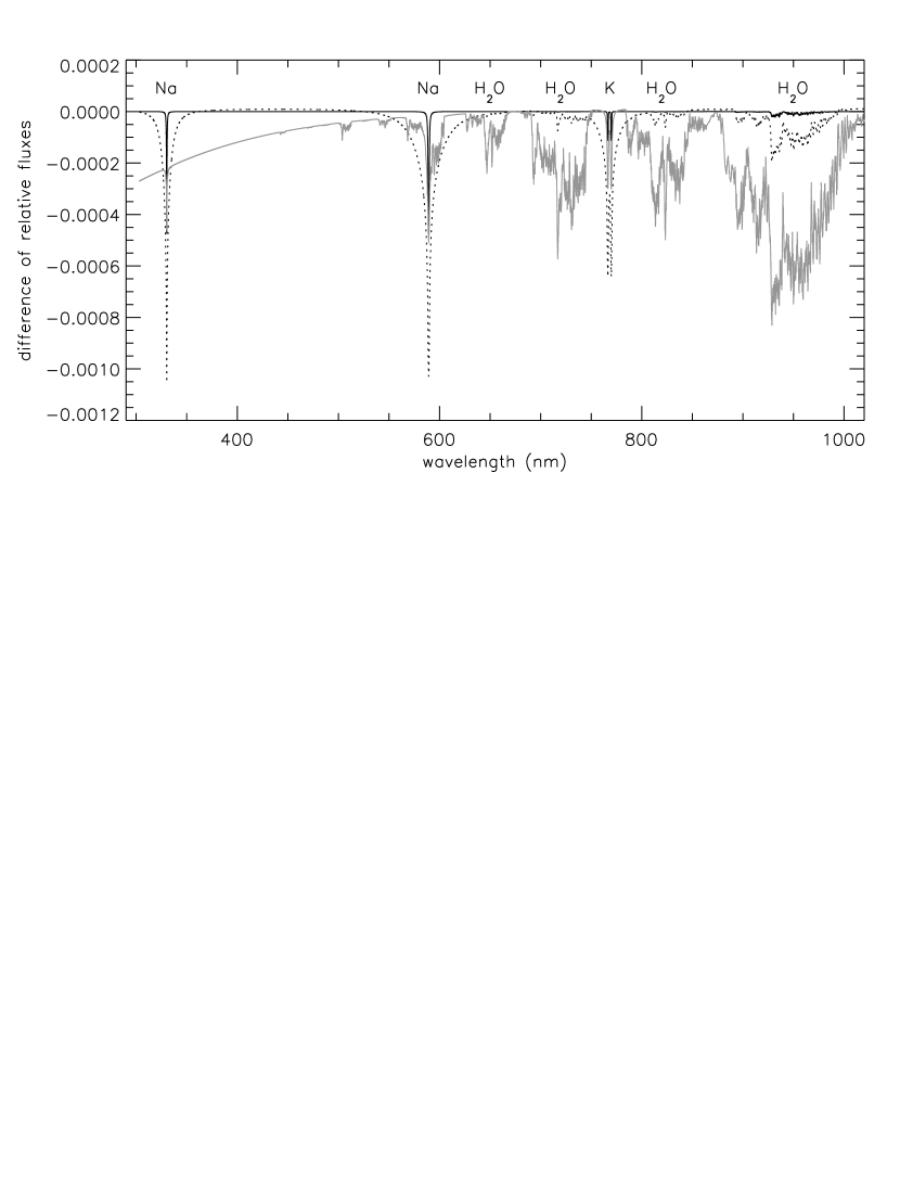
Figure 5: Shown are three model transmission spectra for HD 209458 over a wavelength range that exceeds that of our current data set. The fiducial model (s1) with a solar abundance of sodium, and cloud tops at 0.0368 bar, is shown as a dotted line. This model is excluded by the data, which do not permit such a deep sodium feature. One possibility is that very high clouds reduce the depth of the sodium absorption feature; such a model is shown as the solid line. Another possibility is that the abundance of atomic sodium in the planetary atmosphere is reduced greatly from the solar value; this is shown as the gray line. Observations of the transmission spectrum over the range shown here should allow for us to distinguish between these two broad categories of models.

We investigate the possibility that the observed decrement is due to non-linearity in the STIS CCD: Since the observed value of $\Delta n_{Na}$ is $-2.32\times 10^{-4}$ for a change in mean intensity inside to outside transit of $-1.6\times 10^{-2}$, a non-linearity of $\sim 1$% across this range would be required. Gilliland, Goudfrooij, & Kimble (1999) derive an upper limit that is an order of magnitude lower than this. We further test this effect directly by selecting 18 strong stellar absorption features in our observed wavelength range. For each spectral feature, we define a set of band passes with the same wavelength range as those listed in Table 1, but now centered on the spectral line. We derive $\Delta n$ and $\Delta m$ for each of these as in equation (5). The results are shown in Figure 5. We find no correlation of either $\Delta n$ or $\Delta m$ with spectral line depth. These tests also confirm our evaluation of the precision we achieve in equation (5): We find that the values of $\Delta n$ or $\Delta m$ are normally distributed, with a mean consistent with 0, and a standard deviation as we found above (eq. [5]).

3 Comparison with Theoretical Predictions

As described above, the quantity that we observe is the difference in the transit depth in a band centered on the Na D lines to the average of two flanking bands, as a function of time from the center of transit: We denoted these by $n_{Na}(t)$, $m_{Na}(t)$, and $w_{Na}(t)$, above. We wish to compare these results to models of the planetary atmosphere. Several steps are required to transform the model predictions into the same quantity as the observable, and we describe these steps here.

We first produce several model calculations of the change in the effective planetary radius as a function of wavelength, as prescribed by Brown (2001). For all the models, we use the best-fit values from B01 for $R_{p}$, $R_{s}$, $i$, $a$, $M_{s}$ as given in § 2.1. We further specify the planetary mass ($M_{p}=0.69~{}M_{\rm Jup}$) and the stellar effective temperature ($T_{s}=6000$ K), both as given by Mazeh et al. (2000). We set the equatorial rotational velocity of the planet to $v_{rot}=2.0{\rm\;km\,s^{-1}}$. This is the value implied by the measured planetary radius, under the assumption that the planet is tidally locked (i.e. the rotational period is the same as the orbital period). Each model includes the effect of photoionization as described in Brown (2001), which reduces the core strength of the Na D lines, but does not significantly change the wings.

The fiducial model has a cloud deck with cloud tops at a pressure of .0368 ( = 0.1 / e) bar, and solar metallicity (the measured value for HD 209458; Mazeh et al., 2000). We also consider a number of variants to the fiducial model, representing changes to either the metal abundance, or the cloud height. These variants are listed in Table 2. For each model (denoted by the index $m$), we have the theoretical planetary radius $R_{p}(\lambda,m)$, where $\lambda$ denotes the wavelength. For each of these, we renormalize $R_{p}(\lambda,m)$ so that the average value of the planetary radius over the entire STIS bandpass is the best-fit value determined by B01 ($1.347~{}R_{\rm Jup}$). These renormalized functions $R_{p}(\lambda,m)$ are shown in Figure 6.

We use the theoretical model of the stellar surface brightness [$S(\lambda,\mu)$; described in § 2.1] to include the effects of the wavelength-dependent limb-darkening of the star. This approach allows us to account for both the continuum limb-darkening, and the deviations that occur from this in the cores of absorption lines; these can be significant in the case of the sodium features. In general, the limb-darkening is less pronounced in the cores of the sodium lines than in the adjacent continuum, and thus for a planetary radius that is independent of wavelength, the transit light curve near $T_{c}$ is deeper and more rounded as observed in the continuum than as observed in the core of an absorption line.

We proceed as described in § 2.1, with the exception that $R_{p}(\lambda,m)$ is now a function of wavelength: For each $\lambda$, we produce the theoretical transit curve, $T(\lambda,t,m)$. We bin these results in the wavelength bands as described in § 2, and difference the values in the band centered on the sodium lines from the average of the flanking bands, as prescribed by equation (4). The result is a theoretical time series that closely resembles the observed STIS time series, with the effect of a wavelength-dependent planetary radius included. These model time series are shown in Figure 7, and may be compared directly with the data shown in Figures 2 & 4.

We find that most of the models listed in Table 1 produce differential transits that are significantly deeper than our observational result. Only models n4 or c3, which represent, respectively, extreme values of high cloud height or depleted atomic sodium abundance, produce transits of approximately the correct depth.

4 Discussion

We have detected a significantly deeper transit in the sodium band relative to the adjacent bands. We interpret the signal as due to absorption by sodium in the planetary atmosphere. We are encouraged in this interpretation by the following two considerations: First, a sodium feature in the transmission spectrum of HD 209458 was predicted unanimously by the current modeling efforts (Seager & Sasselov, 2000; Brown, 2001; Hubbard et al., 2001). Second, observed spectra of L-type objects (e.g. Kirkpatrick et al., 1999), T-dwarfs (e.g. Burgasser et al., 1999) and, in particular, the brown dwarf Gl 229 B (e.g. Oppenheimer et al., 1998), show very strong absorption from alkali metal lines (Burrows, Marley, & Sharp, 2000). These objects span a temperature range of 900-2000 K, which includes the equilibrium temperature of HD 209458 b, $T_{eff}=1430~{}(1-A)^{\frac{1}{4}}$ K (where $A$ indicates the Bond albedo). (It should be noted that these objects are at roughly the same temperature as HD 209458 b for very different reasons: The planet is heated by its proximity to the parent star, whereas the temperatures for the other objects are set by their ongoing contraction.)

In the following discussion, we first consider alternate interpretations of our result, then discuss the constraints that we can place on the planetary atmosphere, and finish by looking ahead to near-future complementary observations.

4.1 Alternate Explanations

We must take care that the observed decrement is not the result of the distinctive limb-darkening exhibited by the sodium line relative to that of the adjacent continuum. In order to quantify the amplitude of this effect, we generated model transit curves (for a planet of constant radius) as described in § 2.1, and integrated these in $\lambda$ over the nine band passes listed in Table 1. We then recreated the linear combination of these results as given in eq (4). We found that the predicted offsets were:

$$\begin{array}[]{cccc}\Delta n_{Na}&{\rm(theory;constant}~{}R_{p}{\rm)}&=&+1.52\times 10^{-5}\phantom{string}\\ \Delta m_{Na}&{\rm(theory;constant}~{}R_{p}{\rm)}&=&+0.39\times 10^{-5}\phantom{string}\\ \Delta w_{Na}&{\rm(theory;constant}~{}R_{p}{\rm)}&=&+0.47\times 10^{-5}.\end{array}$$ (6)

These values are much smaller than the signal we detect. Moreover, they are of the opposite sign: Since the net decrement toward the limb is less in the sodium line than in the adjacent continuum, the transit as observed in a band centered on the sodium lines would be expected to be less deep near $T_{c}$ than that observed in a band in the adjacent spectral region. We note that the above quantities should be subtracted from the observed values of $\Delta n_{Na}$, $\Delta m_{Na}$, and $\Delta w_{Na}$ given in equation (5) for comparison with future modeling efforts that do not explicitly include the wavelength-dependent limb-darkening. For the purposes of the present paper, our models explicitly account for this effect by making use of the model stellar surface brightness, and thus no adjustment is needed.

A second concern is that the star might appear smaller when observed at the wavelength of the sodium lines, producing a deeper transit for the same-sized planet. In fact, we expect the opposite to be true: The solar limb should be slightly larger in the core of the Na D lines because of the great opacity in these lines. Model calculations (E. H. Avrett, personal communication) yield an intensity-weighted solar radius increase, after averaging over even the narrowest bandpass containing the Na D lines, of less than 10 km. This will have a completely negligible effect on the observed transit depth in the bandpass containing the Na D lines.

4.2 Constraints on the Planetary Atmosphere

Our fiducial model (s1), which has cloud tops at 0.04 bar and a solar abundance of sodium in atomic form, predicts values for $\Delta n_{Na}$ and $\Delta m_{Na}$ that are $\sim$3 times deeper than we observe. This conclusion awaits confirmation from other more detailed models, such as those performed by Seager & Sasselov (2000) and Hubbard et al. (2001). Here we consider several possible physical effects that may contribute to the reduced sodium absorption relative to the predictions of our model:

It may be that a significant fraction of atomic sodium has combined into molecules, which may either be present as gaseous species, or sequestered from the atmosphere as condensates. Chemical equilibrium models for substellar and planetary atmospheres (Fegley & Lodders, 1994, 1996; Burrows & Sharp, 1999; Lodders, 1999) indicate that Na₂S, NaCl, NaOH, NaH, and more complicated species (such as NaAlSi₃O₈) may be present in the planetary atmosphere. In particular, Lodders (1999) finds that, at these temperatures, the competition for sodium is predominantly between Na₂S (solid) and monatomic Na (gas). At temperatures above the Na₂S-condensation line, sodium is predominantly in atomic form, and gases such as NaCl, NaOH, and NaH never become the most abundant sodium-bearing species (K. Lodders, personal communcation). If the disparity between the observed values for $\Delta n_{Na}$ and $\Delta m_{Na}$ and the predictions for these quantities based on our fiducial model (s1), is due entirely to this effect (and not, for example, mitigated by the effect of high cloud decks), then this would indicate that less than 1 % of the sodium is present in atomic form. This statement is based on the fact that even our model c3 fails to reproduce the observed values.

Our current models (Brown, 2001) account for the ionization of sodium by the large stellar flux incident upon the planetary atmosphere. However, it is possible that the effect is larger than predicted by our calculations: This would require a sink for free electrons, the effect of which would be to lower the recombination rate.

Perhaps HD 209458 began with a depleted sodium abundance, or, more generally, a depleted metal abundance. The current picture of gas-giant planet formation predicts that planets should present a metallicity at or above the value observed in the parent star; Jupiter and Saturn are certainly metal-rich relative to the Sun (see discussion in Fegley & Lodders, 1994). Metallicity appears to play an important role in the formation of planets: Parent stars of close-in planets appear to be metal rich (Gonzalez, 1997, 2000) relative to their counterparts in the local solar neighborhood (Queloz et al., 2000b; Butler et al., 2000). Furthermore, the observed lack of close-in giant planets in the globular cluster 47 Tuc (Gilliland et al., 2000) may be due, in part, to a reduced planet-formation rate due to the low-metallicity of the globular cluster. The relationship linking metallicity and planet formation is not clear.

Clouds provide a natural means of reducing the sodium absorption, by creating a hard edge to the atmosphere, and thereby reducing the effective area of the atmosphere viewed in transmission. If the difference between the observed values of $\Delta n_{Na}$ and $\Delta m_{Na}$ and the predictions for these quantities based on our fiducial model (s1) is due entirely to clouds, then this would require a very high cloud deck, with cloud tops above 0.4 mbar (model n4). Ackerman & Marley (2001) have recently produced algorithms to model cloud formation in the atmospheres of extrasolar planets. The effect of the stellar UV flux on the atmospheric chemistry has not been explicitly included. We urge investigations of the production of condensates, such as photochemical hazes, by this mechanism. Such photochemical hazes are present in the atmospheres of the gas giants of the solar system, and produce large effects upon the observed reflectance spectra of these bodies (Karkoschka, 1994). The stellar flux incident upon the atmosphere of HD 209458 b is roughly 20,000 times greater than that upon Jupiter.

4.3 Future Observations

In the present work, we have demonstrated that by using existing instruments, it is possible to begin the investigation of the atmospheres of planets orbiting other stars. Wide-field surveys conducted by dedicated, small telescopes (e.g. Borucki et al., 2001; Brown & Charbonneau, 2000) promise to detect numerous close-in, transiting planets over the next few years. The parent stars of these planets should be sufficiently bright to permit similar studies of the planetary atmosphere.

Based on the results presented here, we believe the observed value of sodium absorption from the planetary atmosphere may have resulted from a high cloud deck, a low atomic sodium abundance, or a combination of both. Observations of the transmission spectrum over a broader wavelength range should allow us to distinguish between these two broad categories of models (Figure 8). If the effect is predominantly due to clouds, the transmission spectrum from 300–1000 nm will show little variation with wavelength, other than additional alkali metal lines. If, on the other hand, the clouds are very deep or not present, then the transmission spectrum may show deep features redward of 500 nm due to water, and absorption due to Rayleigh scattering blueward of 500 nm. These are only two extremes of the many possibilities; the actual case may share characteristics of both of these effects. Further diagnostics could be provided by near-IR spectroscopy, which could detect features due to molecular species (such as ${\rm H_{2}O}$, CO, and ${\rm CH_{4}}$) that are expected to be present in planetary transmission spectra (Seager & Sasselov, 2000; Brown, 2001; Hubbard et al., 2001). Suitable observations in the 1–5 $\mu$m region would allow inferences about the atmosphere’s thermal structure and composition, permitting a more definite interpretation of the sodium signature. Brown et al. (2000) have presented preliminary near-IR spectra of HD 209458 in and out of transit. These spectra demonstrate that it should be possible to search for near-IR atmospheric signatures with existing instruments, such as the NIRSPEC spectrograph (McLean et al., 1998) on the Keck II telescope.

Observations of the reflected light spectrum (wavelength-dependent geometric albedo) as pursued for the $\tau$ Boo system (Charbonneau et al., 1999; Collier Cameron et al., 1999) would complement the results of transmission spectroscopy. Predictions for the albedo as a function of wavelength vary by several orders of magnitude (Seager & Sasselov, 1998; Marley et al., 1999; Goukenleuque et al., 2000; Sudarsky, Burrows, & Pinto, 2000). These observations should be facilitated in the case of a transiting system (Charbonneau & Noyes, 2000). If possible, the observation of the phase function (variation in the reflected-light with orbital phase) would constrain greatly the nature of particulates in the planetary atmosphere (Seager, Whitney, & Sasselov, 2000). Observations of molecular absorption features from thermal emission spectra, such as sought in the recent study of the $\tau$ Boo system (Wiedemann, Deming, & Bjoraker, 2001), would clearly complement these studies. Finally, infrared photometry of the secondary eclipse would provide a direct measurement of the effective temperature of the planetary atmosphere, should the requisite precision be achieved.

Table 1: Wavelength Bands

width	blue (nm)	center (nm)	red (nm)
narrow	$n_{b}$: 581.8–588.7	$n_{c}$: 588.7–589.9	$n_{r}$: 589.9–596.8
medium	$m_{b}$: 581.8–587.4	$m_{c}$: 587.4–591.2	$m_{r}$: 591.2–596.8
wide	$w_{b}$: 581.8–584.3	$w_{c}$: 584.3–594.3	$w_{r}$: 594.3–596.8

Table 2: Model Atmosphere Parameters

identifier	cloud tops	metal abundance
	(bar)	(relative to solar)
s1	0.036800	1.00
n1	3.680000	1.00
n2	0.368000	1.00
n3	0.003680	1.00
n4	0.000368	1.00
c1	0.036800	2.00
c2	0.036800	0.50
c3	0.036800	0.01

Figure 1: Shown is a portion of a STIS spectrum of HD 209458, centered on the Na D lines. The vertical axis is the number of detected photoelectrons per wavelength pixel after integrating over 17 pixels in cross-dispersion. The vertical lines indicate the band passes over which we integrate the spectrum to produce the photometric time series. The band $n_{c}$ is the set of pixels between the two dotted lines; $m_{c}$ is the set between the dashed lines; $w_{c}$ is the set between the dot-dashed lines. The corresponding blue bands ($n_{b}$, $m_{b}$, and $w_{b}$) are the set of pixels between the left solid line and the left boundary of the center band. Similarly, the corresponding red bands ($n_{r}$, $m_{r}$, and $w_{r}$) are the set of pixels between the right edge of the center band and the right solid line.

(Previous page)  The unbinned time series $n_{Na}$, $m_{Na}$, and $w_{Na}$ are plotted in the top, center, and bottom panels, respectively, as a function of absolute time from the center of transit. The mean of the in-transit values of $n_{Na}$ and $m_{Na}$ are both significantly offset below 0.

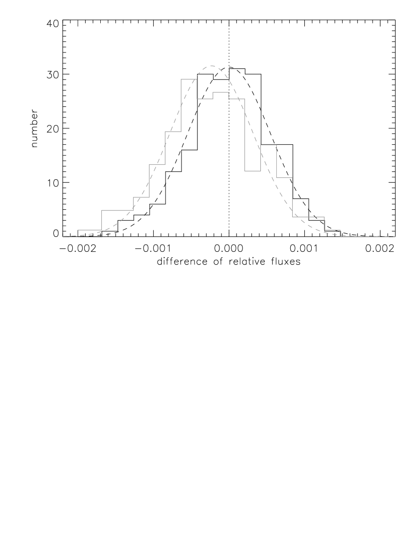
Figure 2: The dark solid line is a histogram of the out-of-transit values of $n_{Na}$ (the data shown in the upper panel of Figure 2). The dashed dark curve is a Gaussian distribution with a mean of 0, $\sigma=5.5\times 10^{-4}$ as prescribed from photon-noise-predictions, and normalized to the same area. The gray solid line is a histogram of the in-transit values of $n_{Na}$, renormalized to the same number of observations as the dark solid line. The dashed gray curve is a Gaussian distribution with the same $\sigma$ as the dark curve, but with a mean of $-2.32\times 10^{-4}$ (the observed value). The gray histogram is significantly offset from 0.

Figure 3: The upper panel shows the unbinned time series $n_{Na}$ (the data shown in the upper panel of Figure 2). The lower panel shows these data binned in time (each point is the median value in each bin). There are 10 bins, with roughly equal numbers of observations per bin (42). The error bars indicate the estimated standard deviation of the median. The solid curve is a model for the difference of two transit curves (described in § 3), scaled to the observed offset in the mean during transit, $\Delta n_{Na}=-2.32\times 10^{-4}$.

(Previous page)  The upper panel shows a typical spectrum of HD 209458, over the full spectroscopic range that we observed. We selected 18 strong features in addition to the Na D lines; these are indicated by vertical dashed lines. The middle panel shows the results for the narrow ($n$) band pass. The black diamond is the value of $\Delta n_{Na}$. The wavelength ranges of the bands $n_{b}$, $n_{c}$, and $n_{r}$ are shown as the horizontal gray bars. We then repeated the analysis, i.e. same band widths, but now centered over each of the 18 features that are indicated. The resulting values are shown as white diamonds. The lower panel shows the corresponding results for the middle ($m$) band pass. In each case, the white diamond points appear to be normally-distributed, with a mean of 0, and a standard deviation as prescribed by photon statistics. In particular, the residuals do not correlate with the depth of the spectral feature. Some correlations between adjacent white points are evident, as expected, since the band passes are wider than the separation between points. In the middle and lower panels, the black diamond point is inconsistent with no variation at the level of 4.1 $\sigma$ and 3.4 $\sigma$, respectively. Note that the y-axis in the lower panel has been scaled so that the error bars appear the same size as in the middle panel.

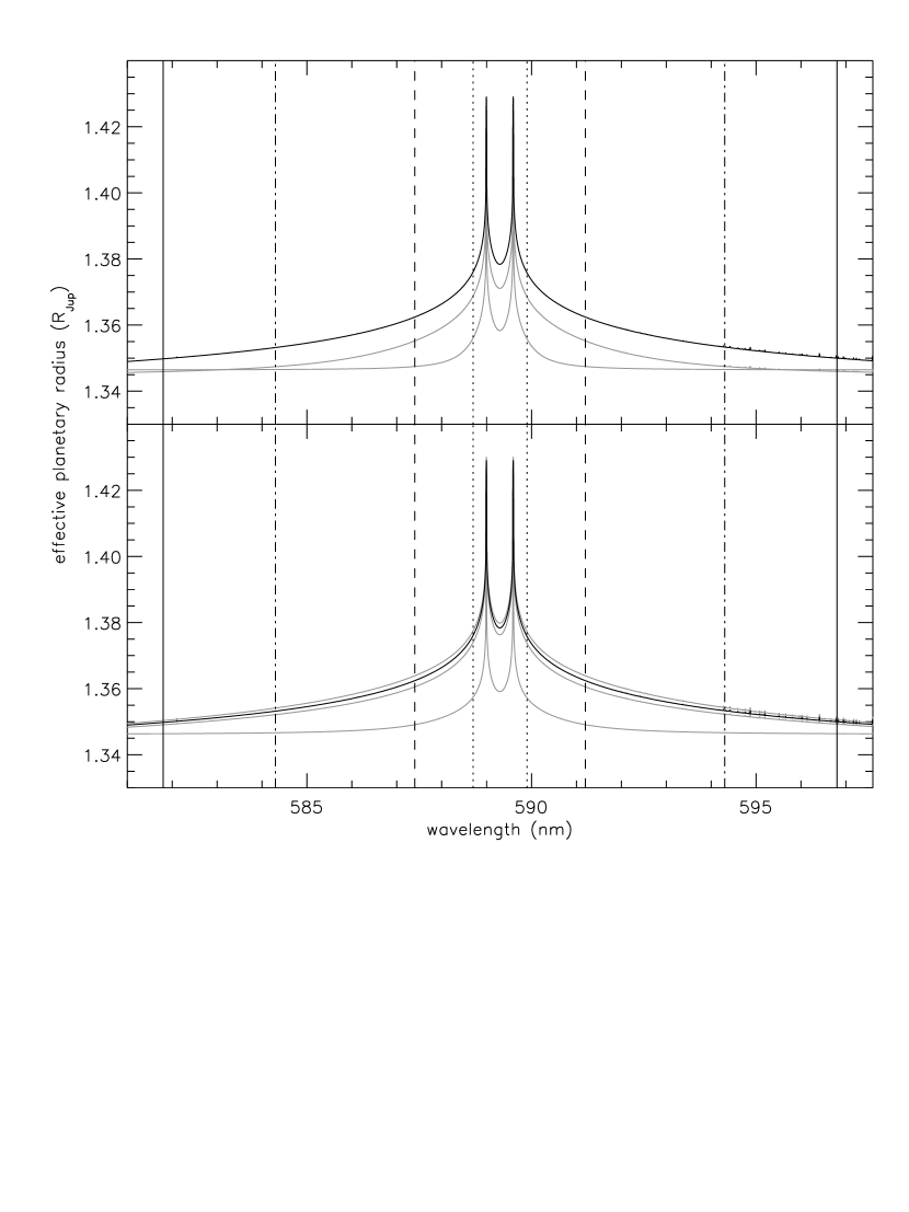
Figure 4: The effective planetary radius is shown as a function of wavelength for a variety of atmospheric models; the vertical lines indicate the bandwidths, and are the same lines as those in Figure 1. In both panels, the dark line shows the planetary radius for the fiducial model (s1). In the upper panel, we show the variation with cloud height; the upper and lower gray curves are models n3 and n4, respectively. (The results for models n1 and n2 are indistinguishable on this plot from that for s1). In the lower panel, we show the variation with sodium abundance; the gray curves are, from top to bottom, models c1, c2, and c3.

(Previous page)  The solid curve in the top panel shows the model curve for $n_{Na}$ for the fiducial model (s1). The solid curves in the middle and lower panels are the results for $m_{Na}$ and $w_{Na}$, respectively, for this same model. The dashed lines show the variations due to cloud height: Within each panel, the upper dashed curve is for model n4, and the lower dashed curve is for model n3. (The results for models n1 and n2 are indistinguishable on this plot from that for s1). The solid gray lines show the variations due to atomic sodium abundance: Within each panel, the gray curves correspond (from top to bottom) to models c3, c2, and c1. These curves may be compared directly with the data presented in Figures 2 and 4.

References

- Ackerman & Marley (2001) Ackerman, A. S. & Marley, M. S. 2001, ApJ, 556, 872
- Borucki et al. (2001) Borucki, W. J., Caldwell, D., Koch, D. G., Webster, L. D., Jenkins, J. M., Ninkov, Z., & Showen, R. 2001, PASP, 113, 439
- Brown (2001) Brown, T. M. 2001, ApJ, 553, 1006
- Brown et al. (2001) Brown, T. M., Charbonneau, D., Gilliland, R. L., Noyes, R. W., & Burrows, A. 2001, ApJ, 552, 699
- Brown & Charbonneau (2000) Brown, T. M. & Charbonneau, D. 2000, in ASP Conf. Ser. 219: Disks, Planetesimals, and Planets, ed. F. Garzón, C. Eiroa, D. de Winter, & T. J. Mahoney (San Francisco: ASP), 557
- Brown et al. (2000) Brown, T. M. et al. 2000, American Astronomical Society Meeting, 197, 1105
- Bundy & Marcy (2000) Bundy, K. A. & Marcy, G. W. 2000, PASP, 112, 1421
- Burgasser et al. (1999) Burgasser, A. J. et al. 1999, ApJ, 522, L65
- Burrows, Marley, & Sharp (2000) Burrows, A., Marley, M. S., & Sharp, C. M. 2000, ApJ, 531, 438
- Burrows & Sharp (1999) Burrows, A. & Sharp, C. M. 1999, ApJ, 512, 843
- Butler et al. (2000) Butler, R. P., Vogt, S. S., Marcy, G. W., Fischer, D. A., Henry, G. W., & Apps, K. 2000, ApJ, 545, 504
- Collier Cameron et al. (1999) Collier Cameron, A., Horne, K., Penny, A., & James, D. 1999, Nature, 402, 751
- Cox (2000) Cox, A. N. 2000, Allen’s Astrophysical Quantities, 4th ed., ed. A. N. Cox, (New York: AIP Press)
- Charbonneau et al. (2000) Charbonneau, D., Brown, T. M., Latham, D. W. & Mayor, M. 2000, ApJ, 529, L45
- Charbonneau & Noyes (2000) Charbonneau, D., & Noyes, R. W. 2000, in ASP Conf. Ser. 219: Disks, Planetesimals, and Planets, ed. F. Garzón, C. Eiroa, D. de Winter, & T. J. Mahoney (San Francisco: ASP), 461
- Charbonneau et al. (1999) Charbonneau, D., Noyes, R. W., Korzennik, S. G., Nisenson, P., Jha, S., Vogt, S. S., & Kibrick, R. I. 1999, ApJ, 522, L145
- Coustenis et al. (1998) Coustenis, A., et al. 1998, ASP Conf. Ser. 134, Brown Dwarfs and Extrasolar Planets, ed. R. Rebolo, E. Matín, & M. R. Zapatero Osorio (San Francisco:ASP), 296
- Deeg, Garrido, & Claret (2001) Deeg, H., Garrido, R. & Claret A. 2001, New Astronomy, 6, 51
- Fegley & Lodders (1994) Fegley, B., Jr., & Lodders, K. 1994, Icarus, 110, 117
- Fegley & Lodders (1996) Fegley, B., Jr., & Lodders, K. 1996, ApJ, 472, L37
- Gilliland, Goudfrooij, & Kimble (1999) Gilliland, R. L., Goudfrooij, P., & Kimble, R. A. 1999, PASP, 111, 1009
- Gilliland et al. (2000) Gilliland, R. L. et al. 2000, ApJ, 545, L47
- Gonzalez (1997) Gonzalez, G. 1997, MNRAS, 285, 403
- Gonzalez (2000) Gonzalez, G. 2000, in ASP Conf. Ser. 219: Disks, Planetesimals, and Planets, ed. F. Garzón, C. Eiroa, D. de Winter, & T. J. Mahoney (San Francisco: ASP), 523
- Goukenleuque et al. (2000) Goukenleuque, C., Bézard, B., Joguet, B., Lellouch, E., & Freedman, R. 2000, Icarus, 143, 308
- Henry et al. (2000) Henry, G. W., Marcy, G. W., Butler, R. P., & Vogt, S. S. 2000, ApJ, 529, L41
- Hubbard et al. (2001) Hubbard, W. B., Fortney, J. J., Lunine, J. I., Burrows, A., Sudarsky, D., & Pinto, P. A. 2001, ApJ, 560, 413
- Jha et al. (2000) Jha, S., Charbonneau, D., Garnavich, P. M., Sullivan, D. J., Sullivan, T., Brown, T. M., & Tonry, J. L. 2000, ApJ, 540, L45
- Karkoschka (1994) Karkoschka, E. 1994, Icarus, 111, 174
- Kirkpatrick et al. (1999) Kirkpatrick, J. D. et al. 1999, ApJ, 519, 802
- Lodders (1999) Lodders, K. 1999, ApJ, 519, 793
- Marley et al. (1999) Marley, M. S., Gelino, C., Stephens, D., Lunine, J. I., & Freedman, R. 1999, ApJ, 513, 879
- Mazeh et al. (2000) Mazeh, T., et al. 2000, ApJ, 532, L55
- McLean et al. (1998) McLean, I. S. et al. 1998, Proc. SPIE, 3354, 566
- Moutou et al. (2001) Moutou, C., Coustenis, A., Schneider, J., St Gilles, R., Mayor, M., Queloz, D., & Kaufer, A. 2001, A&A, 371, 260
- Oppenheimer et al. (1998) Oppenheimer, B. R., Kulkarni, S. R., Matthews, K., & van Kerkwijk, M. H. 1998, ApJ, 502, 932
- Queloz et al. (2000) Queloz, D., Eggenberger, A., Mayor, M., Perrier, C., Beuzit, J. L., Naef, D., Sivan, J. P., & Udry, S. 2000, A&A, 359, L13
- Queloz et al. (2000b) Queloz, D. et al. 2000, A&A, 354, 99
- Rauer et al. (2000) Rauer, H., Bockelée-Morvan, D., Coustenis, A., Guillot, T., & Schneider, J. 2000, A&A, 355, 573
- Sackett (1999) Sackett, P. D. 1999, NATO ASIC Proc. 532: Planets Outside the Solar System: Theory and Observations, 189
- Seager & Sasselov (1998) Seager, S. & Sasselov, D. D. 1998, ApJ, 502, L157
- Seager & Sasselov (2000) Seager, S. & Sasselov, D. D. 2000, ApJ, 537, 916
- Seager, Whitney, & Sasselov (2000) Seager, S., Whitney, B. A., & Sasselov, D. D. 2000, ApJ, 540, 504
- Sudarsky, Burrows, & Pinto (2000) Sudarsky, D., Burrows, A., & Pinto, P. 2000, ApJ, 538, 885
- Wiedemann, Deming, & Bjoraker (2001) Wiedemann, G., Deming, D., & Bjoraker, G. 2001, ApJ, 546, 1068