Deep Westerbork 1.4 GHz Imaging of the Bootes Field

Abstract

We present the results from our deep (16$\times$12 hour) Westerbork Synthesis Radio Telescope (WSRT) observations of the approximately 7 square degree Bootes Deep Field, centered at $14^{\rm h}32^{\rm m}05\fs 75$, $34\arcdeg 16\arcmin 47\farcs 5$ (J2000). Our survey consists of 42 discrete pointings, with enough overlap to ensure a uniform sensitivity across the entire field, with a limiting sensitivity of 28$\mu$Jy (1$\sigma_{\mbox{rms}}$). The catalog contains 3172 distinct sources, of which 316 are resolved by the $13\arcsec\times 27\arcsec$ beam. The Bootes field is part of the optical/near-infrared imaging and spectroscopy survey effort conducted at various institutions. The combination of these data sets, and the deep nature of the radio observations will allow unique studies of a large range of topics including the redshift evolution of the luminosity function of radio sources, the K-$z$ relation and the clustering environment of radio galaxies, the radio / far-infrared correlation for distant starbursts, and the nature of obscured radio loud AGN.

1 Introduction

One of the main goals of radio astronomy is to fully understand the physics of the population of extragalactic radio sources (RSs). Issues include the onset and demise of the radio activity and related starbursts, the influence of the environment on the characteristics of the RSs and the appearance of the first RSs and their relation to the formation of galaxies, massive black holes and the reionization of the universe.

Detailed investigation of complete samples of bright RSs with redshift information have been carried out over the last decades (e.g., 3CRR: Laing, Riley & Longair 1983; 6CE: Eales 1985, Eales et al. 1997, Rawlings, Eales & Lacy 2001) and led to many interesting discoveries. For example, it is now well established that the comoving number density of $z\approx 1$ powerful RSs is about two orders of magnitude larger than it is locally (e.g., Longair 1966, Dunlop & Peacock 1990). Another example is that the environment of RSs changes with redshift, with bright RSs at higher redshifts located in denser environments than locally (e.g., Best, Longair & Röttgering 1998).

Through the selection of RSs that are bright and have very steep radio spectra ($<-1.3$), more than 150 powerful galaxies with $2<z<5.2$ have been found (De Breuck et al., 2000). The large starformation rates (Dey et al., 1997) and extremely clumpy optical/IR morphologies (Penterrici et al., 1999) provide strong evidence that these galaxies are massive galaxies close to the epoch of formation. Powerful radio emission is most likely caused by accretion onto massive black holes (M${}_{\rm BH}>10^{9}$ M_☉; McLure et al. 1999, Laor 2000), indicating that such massive black holes formed alongside or possibly before the formation epoch of their host galaxies (e.g., Kauffmann & Haehnelt 2000). Recent VLT observations have revealed the existence of a large scale structure of Ly-$\alpha$ emitting galaxies around the radio galaxy 1138$-$262 ($z=2.2$), reinforcing the idea that high redshift radio galaxies (HzRGs) can be used as tracers of proto-clusters of galaxies (Pentericci et al., 2000).

At very faint flux densities (e.g., a few tens of $\mu$Jy at 1.4 GHz) the radio source counts are dominated by the $z\lesssim 1$ starburst population (e.g., Richards et al. 1999). Long observations with the VLA + MERLIN (Richards, 2000; Muxlow et al., 1999) and WSRT (Garrett et al., 2000) reach such faint levels, and have enabled important constraints to be placed upon the redshifts and nature of distant starburst galaxies.

1.1 Survey Rationale

Figure 1: Composition of the radio source population as function of 325 MHz flux. The fraction of flat spectrum sources increases dramatically with decreasing flux, whereas the steep spectrum component (dominated by AGN) drops precipitously. Data are from the source overlap between the WENSS and NVSS surveys, at 325 and 1400 MHz respectively. The errorbars represent Poissonian errors, and may be smaller than the symbol size in some cases. Note that WENSS sample incompleteness sets in around 20 mJy, affecting the steep source count most.

Our WSRT survey reaches a 1$\sigma$ detection threshold of 28 $\mu$Jy at 1.4 GHz, within a factor of 2-3 of the deepest radio observations carried out so far (cf. Windhorst et al. 1999, Richards 2000). The surveyed area is, however, large enough (about 7 square degrees) to yield enough sources to not be severely affected by low number statistics for the RS populations under scrutiny. As can be seen in Fig. 1, the composition of the radio population changes dramatically towards lower flux density limits. The higher flux levels are dominated by RSs with steep spectra ($<-0.5$), and a cross-over to flat-spectrum sources appears to occur at the 10-100 mJy (at 325 MHz) level. The former are mostly identified with (powerful) radio sources residing in massive ellipticals (e.g., Eales et al. 1997), whereas the latter can be tied to a population of starforming late-type galaxies, especially towards sub-mJy 1.4 GHz flux density levels (e.g., Windhorst 1999, Richards et al. 1999). Therefore, deeper observations will not only increase the number of detected sources, but it will also provide a better handle on the relative makeup of the radio population at $\mu$Jy  flux density levels.

Figure 2: Expected redshift distribution of the radio source population for our survey, based on the luminosity functions of Dunlop & Peacock (1990, PLE model), and Hopkins et al. (1998, the Phoenix survey).

The radio source population properties do not only change as a function of flux density, they also vary with redshift. Using radio luminosity functions for AGN (Dunlop & Peacock, 1990) and starbursting populations (Hopkins et al., 1998), we can model the expected source counts for a given redshift (and limiting flux density). This is plotted in Fig. 2 for a limiting flux density of 140$\mu$Jy. Beyond a redshift of $z\sim 0.3$ the number counts for our survey are expected to be dominated by the AGN population. The combination of information presented in Figs. 1 and 2 makes it clear how dependent on limiting flux density a perceived radio source population is. Indeed, for a limiting flux density of 1 mJy (at 1.4 GHz) the population is dominated by AGN-type sources at all redshifts (Hopkins et al., 1998).

The survey can detect radio sources at the FR I / FR II break level (10²⁵ W Hz^-1 at 1400 MHz, Owen & White 1991) out to a redshift of $z\sim 3$. Fainter FR I type sources with a mean radio power of 10²⁴ W Hz^-1 drop out of the sample around $z\approx 1$, and the much fainter starforming systems will not be detected beyond $z\sim 0.15$ at the 10²² W Hz^-1 level. The local starbursting system M82 has, for comparison, a radio spectral power of $10^{21.99}$ W Hz^-1, given its 1400 MHz flux density of 8.363 Jy (White & Becker, 1992) and the adopted cosmology. Thus the survey provides ample data for evolutionary studies of radio loud systems out to at least a redshift of 1, whereas a more complete census of radio sources down to the spiral / starburst level has to be limited to sources within $z\sim 0.1$.

1.2 Relation to non-Radio Surveys

Key ingredients for follow-up studies are optical / near-infrared identifications and redshift information for at least a large fraction of the radio sources. For this purpose a number of other surveys are either being carried out or are planned for the same part of the sky. These include:

The NOAO Deep Wide-Field Survey (PI’s Jannuzi and Dey). This survey consists of a Northern and a Southern part, with the former field located in Bootes (near the North Galactic Pole), covering a $3\times 3$ degree region, and the latter located in a $2\times 4.5$ degree equatorial region in Cetus. Both fields have been selected for their low mid- to far-infrared cirrus emission, their low H I column densities and the availability of high resolution ($\sim 5\arcsec$) VLA – FIRST survey radio data. Of particular interest to our program is the Bootes field, which will be imaged to a limiting surface brightness of about 28^th magnitude per square arcsecond in $B$, $V$, and $R$, and down to $\sim 22^{\rm nd}$ magnitude per square arcsec in $J$, $H$, and $K$. These detection limits will permit the optical and near-infrared study of faint, sub-L_∗ galaxies out to redshifts of about unity (an L_∗ galaxy will have $K=19.82$ at $z=1$, based on an absolute magnitude of $K=-24.44\pm 0.06$, cf. Kochanek et al. 2001). The typical host galaxies of luminous radio sources, with masses well in excess of L_∗ galaxies, can be detected out to very large redshifts (based on the $K-z$ diagram, e.g., Jarvis et al. 2001, De Breuck et al. 2002). Given our radio source population mix of powerful radio sources associated with intrinsically bright galaxies at high redshift and less luminous starforming systems at much lower redshifts, we expect to be able to detect optical / near-infrared counterparts for most of them. The NOAO survey limits are well matched to our expected counterpart population.

The IRAC Shallow Survey (PI. Eisenhardt). The Bootes field will be covered by SIRTF’s InfraRed Array Camera (IRAC) in four IR bands ranging from 3.6$\mu$m to 8$\mu$m. Coverage towards the longer IR bands up to 160$\mu$m will be provided by the Multiband Imaging Photometer (MIPS), and some spectroscopy by the InfraRed Spectrograph (IRS, PI in both cases is J. Houck).

The NOAO and SIRTF wide field surveys are aimed to study, among other things, (i) the evolution of large-scale structure from $z\sim 1-4$, (ii) the formation and evolution of ellipticals and starforming galaxies, and (iii) the detection of very distant ($z>4$) young galaxies and quasars. The SIRTF IRAC and MIPS observations will also detect star-forming galaxies at mid- to far-infrared wavelengths. It is this multi-wavelength aspect of the project, covering a large fraction of the electromagnetic spectrum (2 radio frequencies, several optical and near-infrared bands, and the mid- to far-infrared space based SIRTF observations) that distinguishes this effort from other deep radio-optical/near-infrared surveys like the Phoenix survey, (Hopkins et al., 1998; Georgakakis et al., 1999), and the Australia Telescope ESO Slice Project (ATESP) (Prandoni et al., 2000a, b, 2001).

1.3 Relation to other Radio Surveys

Figure 3: Comparison between the various radio surveys covering the Bootes field. The triangles represent literature surveys, and the stars are our Bootes WSRT and VLA surveys. Overplotted are representative radio spectra with varying spectral indices: $\alpha=-0.25,-0.75,\mbox{and}-1.25$, for flat-, normal-, and steep-spectrum radio sources. Any given radio source in the VLA-BF survey with a slopes shallower than $-1.25$ should also be present in WSRT-BF. On the other hand, of the sources in WSRT-BF fainter than the VLA-BF limit ($\sim 0.5$ mJy), only the objects with slopes steeper than $-1.25$ should be present in VLA-BF.

The Bootes field has been covered by previous radio surveys, most notably by the Westerbork Northern Sky Survey (WENSS, Rengelink et al. 1997) at 325 MHz, by the NRAO VLA Sky Survey (NVSS, Condon et al. 1998), and by the Faint Images of The Radio Sky at Twenty-cm survey (FIRST, Becker et al. 1995), both at 1.4 GHz. A comparison between the literature surveys and our Bootes surveys (WSRT at 1.4 GHz in this paper, and VLA 325 MHz) is shown in Fig. 3, and tabulated in Table 1. The varying survey depths and frequencies make combining catalogs to obtain spectral index information less than straightforward. For instance, combining NVSS and 87GB (at 5 GHz, Gregory & Condon 1991) only makes sense if one is interested in radio sources with strongly inverted spectra. For our purpose, since the bulk of the radio source population has a spectral index of around $-0.75$ (cf. Fig. 10), a combination of surveys like the WENSS and NVSS / FIRST is best, as can be inferred from the overplotted common radio spectra in Fig. 3.

However, these surveys do not go deep enough to effectively probe the transition in radio source population occurring around the 1 mJy level (cf. Figs. 1, 9, and, e.g., Windhorst et al. 1999). Our WSRT observations do go deep enough, but will need low frequency data of matching sensitivity. We use the VLA at 325 MHz for this purpose, and the data from this program will be described in an subsequent paper. However, both the NVSS and FIRST survey data have been used to calibrate our survey flux densities and positions (cf. Sections 4.1 and 4.2).

2 Observations

The observations were carried out by the Westerbork Synthesis Radio Telescope (WSRT) operating at 1.380 GHz. The WSRT consists of 14 25m telescopes, arranged in a 2.7km East-West configuration. As the back-end, we used the Digital Continuum Backend (DCB) with 8 sub-bands of 10 MHz bandwidth each. The smallest baseline (9$-$A) was set to 54m to limit shadowing at the expense of a reduction in large spatial structure sensitivity ($\sim 800\arcsec$ for this minimum baseline and frequency).

2.1 Field Layout and Instrumental Setup

We designed a survey layout consisting of 42 discrete pointings. The separation between the grid points was chosen to be 60% of the FWHM of the primary beam. Given the used tiling and the known attenuation of the beam, a more or less uniform noise-background is obtained with this spacing (85% of the survey area has a local rms within $\sqrt{2}\sigma_{\mbox{\tiny median}}$, cf. Sect 4.3 and Fig. 8). This strategy is similar to the one used for the Australia Telescope Compact Array (ATCA) ATESP survey (see Prandoni et al. 2000a for a detailed description). The total number of pointings (42) was dictated by the need to cover the 325 MHz VLA primary beam with a uniform sensitivity (noise) level.

During each observing block of 12 hours, the telescopes were continuously cycled between 3 individual grid positions. This “mosaicing” mode (Kolkman, 1993) allows multiple fields to be observed, while still retaining a 12 hour $uv$-coverage for the fields individually (albeit sampled non-continuously). The basic integration time for the observations is 10 seconds. A typical observing cycle can be broken down to a 10s slew-time between the grid positions, and $5\times 10$s on-source time. Even though the net slewing time is less than 10s, some extra time is needed for the array to settle itself after the move. The observing efficiency with this scheme is therefore 83.3%  resulting in $3\times 200^{\rm m}$ net observing time per 12 hour cycle. Given the total allocated time for this project (192 hours), we used the remaining two 12 hour blocks to cycle through all 42 positions. In this setup, each position was revisited every 42 minutes (instead of every 3 minutes), resulting in a rather sparse $uv$-sampling and less than $15^{\rm m}$ on-source time per block.

Each 12 hour block was sandwiched between two phase and polarization calibrators, typically 3C 286 and 3C 147, more than adequate given the system stability. A log of the observations can be obtained from the ftp-site (cf. Sect 4).

3 Reduction

The mosaic was reduced, calibrated, and assembled using the MIRIAD (Sault et al., 1995) software package. The data was typically of high quality, and only a few percent had to be flagged. Usually the bad data was concentrated in channel 5 (of the 8), which, around 1380 MHz, is the frequency band most affected by interference due to the Global Positioning System. Every field pointing was mapped using a multi frequency synthesis approach, where the measurements of the 8 bands individually are gridded simultaneously in the uv plane. This significantly reduces bandwidth smearing problems. Then a three step iterative phase self-calibration cycle was used, using typically around 100 000 clean iterations. The clean was done down to the 3 sigma level, so as not to incorporate too much flux in faint sources that does not belong there. In the few fields with strong sources present we performed amplitude self calibration as well, in all other cases this did not improve the final outcome. In the fourth, and final cycle, spectral index effects on beam-shape were taken into account (Sault & Conway, 1999). The final maps improved significantly by correcting for the small primary beam shape variations across the 8 10 MHz wide frequency channels.

After all the field pointings were reduced in this manner, they were assembled into a final mosaic. This step basically adds up the maps after performing the proper primary beam correction. Since the dirty beam changes slightly across the field, we restored all the data with a fixed synthesized beam of $13.0\arcsec\times 27.0\arcsec$, at a position angle of zero degrees. The mosaic was then further mapped onto $4\arcsec\times 4\arcsec$ pixels, for a total of $\sim 2750^{2}$ pixels.

4 Results

We used automated routines for the source extraction and catalog creation. These were slightly modified from their WENSS counterparts, but the applied methods are exactly the same, all of which are described in detail in Rengelink et al. (1997).

The software works on rectangular patches of sky only, so we tiled the circular overall shape of the survey into three rectangular areas, as outlined in Fig. 8. All of the low noise areas have been included this way, and only a few parts of the noisy edges have not been cataloged. The total cataloged survey area covers 6.68 square degrees.

Part of the catalog, to illustrate its format, has been listed in Table 2. The full version (with 3172 sources) can be obtained through anonymous ftp to ftp://ftp.nfra.nl/pub/Bootes. The complete mosaic, individual pointing maps, and tables with various additional data are available from the same address, all of which are described in the README file.

4.1 Flux Accuracy and Error Estimates

Figure 4: Flux density comparison between sources in common to NVSS and WSRT. Only unresolved WSRT sources (and hence unresolved in NVSS) have been included. The increase in NVSS flux density relative to the WSRT close to its detection limit is possibly due a combination of Malmquist and NVSS clean biases. Errorbars are 1$\sigma$ errors, and may be smaller than the symbol size in some cases.

Figure 5: Relative flux density errors, as function of Signal-to-Noise ratio. WSRT fluxes are compared to NVSS fluxes for unresolved radio sources present in both catalogs. The overplotted solid lines are expected upper and lower envelopes to the flux density fraction, assuming values for $C_{1}$ and $C_{2}$ (cf. Eqn. 3) of $0.04$ and $1.3$ respectively. The dashed lines are for $C_{1}=0.0$ and $C_{2}=2.0$, and illustrate that $C_{1}$ is most dominant at high SNR  while $C_{2}$ is it at low SNR.

We have compared the flux densities of unresolved sources present in both our uncalibrated Bootes and the NVSS catalog. Since the resolution of NVSS (at 45″) is slightly worse than ours ($13\arcsec\times 27\arcsec$), a source which is unresolved in our catalog is consequently unresolved in NVSS. While we could compare our fluxes to the deeper FIRST data, the latter’s much higher angular resolution typically resolves point sources in our catalog, making a direct comparison difficult. The results of the comparison are plotted in Fig. 4. It is clear from the plot that our uncalibrated fluxes are a little too high in comparison to the NVSS fluxes, at least for $S>10$ mJy. Below these fluxes, the NVSS values are systematically too high, and are presumably due to a combination of Malmquist and clean biases. This overestimate of NVSS fluxes close to their detection limit ($\sim 2.5$ mJy) is also evident in the Condon et al. (1998) comparison of NVSS fluxes to deep WSRT (Katgert-Merkelijn et al., 1985) flux densities, cf. Fig. 31 in Condon et al. (1998). Also, Prandoni et al. (2000b) noticed the same effect in comparing their ATCA radio survey fluxes to the NVSS values.

Using flux density weighting, we calculated the offset to be $4.5\pm 3.0$% too high. We reduced our fluxes accordingly (cf. Fig. 5). Following Rengelink et al. (1997), the relative flux density errors can be written as:

$$\frac{\sigma_{S}}{S}=\left(C_{1}^{2}+C_{2}^{2}\left(\frac{\sigma_{\mbox{rms}}}{S}\right)^{2}\right)^{\frac{1}{2}}$$ (1)

This equation reflects the two components of the measurement error, with $C_{1}$ due to a constant systematic error, and $C_{2}$ being dependent on the Signal-to-Noise Ratio (SNR). Ideally, one would like to compare our measured (and corrected) fluxes to their true values in order to determine the constants $C_{1}$ and $C_{2}$ which best fit the observed $S_{\tiny\mbox{WSRT}}/S_{\tiny\mbox{true}}$ ratio. Unfortunately, we do not have such a control data set, instead we use the NVSS measurements. If we assume that the NVSS measurements have a similar error dependence, we can define the flux density ratio as:

$$\frac{S_{\tiny\mbox{WSRT}}}{S_{\tiny\mbox{NVSS}}}=\frac{1\pm\left(C_{1}^{2}+C_{2}^{2}\left(\frac{\sigma_{\tiny\mbox{WSRT}}}{S_{\tiny\mbox{true}}}\right)^{2}\right)^{\frac{1}{2}}}{1\pm\left(C_{1}^{2}+C_{2}^{2}\left(\frac{\sigma_{\tiny\mbox{NVSS}}}{S_{\tiny\mbox{true}}}\right)^{2}\right)^{\frac{1}{2}}}$$ (2)

with $\sigma_{\tiny\mbox{WSRT}}$ and $\sigma_{\tiny\mbox{NVSS}}$ being the median noise in the sky, and $S_{\tiny\mbox{true}}$ the true value of the source flux. The $\sigma$’s are quoted as $0.45$ mJy for the NVSS (Condon et al., 1998), and $0.028$ mJy for our survey. If we further assume that $S_{\tiny\mbox{WSRT}}$ and $S_{\tiny\mbox{NVSS}}$ are approximately equal to $S_{\tiny\mbox{true}}$, and that $\mbox{SNR}_{X}=S_{X}/\sigma_{X}$ with $X$ being either WSRT or NVSS, we can rewrite Eqn. 2 as:

$$\frac{S_{\tiny\mbox{WSRT}}}{S_{\tiny\mbox{NVSS}}}=\frac{1\pm\left(C_{1}^{2}+\left(\frac{C_{2}}{{\tiny\mbox{SNR}}}\right)^{2}\right)^{\frac{1}{2}}}{1\pm\left(C_{1}^{2}+\left(\frac{16.1\times C_{2}}{{\tiny\mbox{SNR}}}\right)^{2}\right)^{\frac{1}{2}}}$$ (3)

based on $\sigma_{\tiny\mbox{NVSS}}=16.1\times\sigma_{\tiny\mbox{WSRT}}$, which implies $\mbox{SNR}_{\tiny\mbox{WSRT}}=16.1\times\mbox{SNR}_{\tiny\mbox{NVSS}}$. The results using Eqn 3 has been overplotted on Fig. 5 such that the maximum (upper) envelope is given by setting the $\pm$ to $1+()/1-()$, and the minimum envelope by $1-()/1+()$ in the equation. The $C$ parameters have been set to $0.04$ and $1.3$ respectively, identical to the values in Rengelink et al. (1997). The model is most sensitive to the $C_{1}$ value, which basically sets the envelope separation at high SNR. The $C_{2}$ value, which scales the SNR dependence is far less constrained. Values of $C_{2}=2$ (e.g., Kaper et al. 1966) are not excluded. Given the assumptions and the assumed uncertainties about the NVSS errors, we adopt the WENSS values of $0.04$ and $1.3$. The quoted flux density errors in the final catalog are calculated with these particular values.

Figure 6: WSRT positional check against FIRST and optical APM positions. Only WSRT point sources are used. FIRST positions are indicated by the solid circles, and APM identifications are potted as open circles. The larger scatter in the APM correlation is due to the association of radio positions with unrelated nearby optical objects. The mean offsets (indicated by the crosses) are $\Delta$RA$=+0.60\arcsec$, $\Delta$DEC$=-0.17\arcsec$ for FIRST  and $\Delta$RA$=+0.51\arcsec$, $\Delta$DEC$=+0.02\arcsec$ for the APM match.

Figure 7: Positional offsets from FIRST / APM positions as a function of the signal-to-noise ratio (SNR). Overplotted as solid squares are the 67 percentile values for a given SNR. The bottom curve represents the best fitting 1$\sigma$ error envelope (cf. Eqn. 4, with $C_{1}=0.44$ and $C_{2}=5.5$. The top curve is identical to the one modeled for the WENSS survey (Rengelink et al. 1997).

4.2 Positional Accuracy

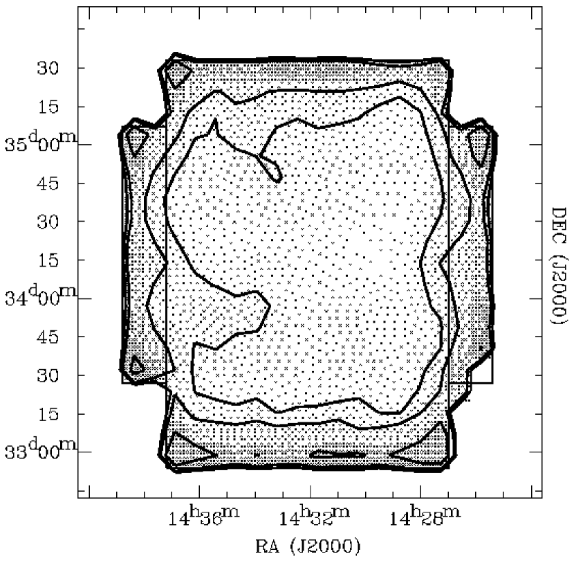
Figure 8: Map of the rms noise inside the source extraction area (outlined by the boxes). The noise levels and relative surface area are, from inside out: $20-30$$\mu$Jy (60.9%), $30-40$$\mu$Jy (23.9%), $40-80$$\mu$Jy (13.3%), and $80-160$$\mu$Jy (2.0%).

Optical identifications can only be securely made if the radio positions are known accurately. The optical source density becomes high enough towards fainter magnitudes to effectively have one potential counterpart per beam. For instance, the mean source separation in the Deeprange $I$-band field survey is about $17\arcsec$ at the 23^rd magnitude level (Postman et al., 1998). This separation is actually smaller than the WSRT beam size at 1400 MHz. Good positional matches are therefore essential.

We compared the cataloged positions for point sources against their FIRST positions and against Automatic Plate Measuring (APM) machine identifications. The APM facility (in Cambridge, UK) catalogs identifications and positions based on scanned UK and POSS II Schmidt plates, covering currently more than 15 000 square degrees of sky.

The relative offsets for the individual sources are plotted in Fig. 6. It is clear that the FIRST and APM positions agree rather well with each other (indicated by the crosses), but that our positions are systematically off in RA. Without more frequent observations of additional calibrators, which would adversely affect our uv coverage, astrometric accuracy of the WSRT is known not to be better than about $0.5\arcsec$ (e.g., Oort & Windhorst 1985), consistent with our offset value. We corrected all the positions in RA with $-0.56\arcsec$, i.e., the mean of the FIRST and APM RA offsets. This correction corresponds to about 4% of the beam width, small but significant enough when accurate positional coincidences are needed.

Analogously to Eqn. 1 for the flux density errors, we can describe the flux density dependence on positional accuracy in the form:

$$\sigma_{\alpha,\delta} = \left(C^{2}_{1}+C^{2}_{2}\left(\frac{\sigma_{\mbox{rms}}}{S}\right)^{2}\right)^{\frac{1}{2}}$$ (4)

$$= \left(C^{2}_{1}+C^{2}_{2}\left(\mbox{SNR}\right)^{-2}\right)^{\frac{1}{2}}$$

The absolute distances from the FIRST positions have been plotted in Fig. 7 as a function of signal-to-noise. Our survey positions have been corrected for the RA offset first. Since the FIRST resolution is higher than our survey and may lead to 2 (or more) FIRST catalog positions for any of our positions, we only considered FIRST point sources within our survey field. The inclusion of resolved sources (either in FIRST or our survey) unnecessarily complicates the comparison.

In Fig. 7 a clear decrease in positional offset with increasing SNR can be seen. To characterize this trend, we fitted Eqn. 4 to the 67th percentile points (solid squares) in order to get a 1$\sigma$ positional error estimate. The best fitting values for the constants are: $C_{1}=0.44$ and $C_{2}=5.5$, both in arcseconds. An outer envelope to the offset distribution is given by $C_{1}=0.44$ and $C_{2}=15.0$. The value for $C_{2}$ is actually the mean beam size (taken to be 20″) divided by 1.3, a value identical to the one quoted for the WENSS survey (Rengelink et al., 1997). We adopt the first set of constants (the 1$\sigma$ equivalents) for our source catalog.

4.3 Completeness and Reliability

The background noise in our survey is not uniformly flat, but has a marked upturn towards the edges. The tiling was set up in such a way that in the interior regions the noise should be flat. This can be verified in Fig. 8, which plots the actual background noise. The median noise level of the inner parts is 28$\mu$Jy. The large 30 to 40$\mu$Jy “intrusion” at 14^h36^m, 34^d00^m is most likely due to the somewhat higher noise levels in those four particular pointings.

Figure 9: Differential source counts as function of flux density $S$ (vertical bars). The counts have been normalized to the expected number for a Euclidean universe. The lengths of the vertical bars are set by the $\sqrt{N}$ error-bars. Overplotted are the differential source counts for the NVSS (stars) and FIRST (open squares) surveys. Note the onset of incompleteness in NVSS at 12 mJy, in FIRST around 2 mJy, and in our survey at about 0.2 mJy.

The survey completeness can be gleaned from Fig. 9, in which the differential source counts are plotted against flux. The number counts have been normalized by the expected number in a Euclidean universe, given by $N_{\mbox{Eucl}}=K_{\nu}S_{\nu}^{-5/2}$, with the unitless constant $K_{\nu}=225$ (consistent with e.g., Oort & Windhorst 1985 and Oort 1987, but see Wall (1994) who lists $K_{\nu}=200$, however). Our source counts are compared to the ones based on the NVSS and FIRST catalogs, which due to their much larger survey area extend further towards higher flux densities. There is good agreement (within the 1$\sigma$ errorbars) over the range 10 – 100 mJy between the surveys. The small deviation in our differential counts around the 4 mJy bin appears to be real and might indicate the presence of an overdense region within our field (e.g., a cluster). Since our survey field is relatively small at 6.68 square degrees, any local overdensity could skew the number counts significantly. The NVSS and FIRST number counts are not affected by this, and serve as a useful baseline.

All three plotted surveys have different completeness limits, and if one marks the first systematic deviation from a low-order polynomial fit as the completeness limit, we measure 12 mJy for NVSS, 2 mJy for FIRST, and 0.2 mJy for our survey. However, since the noise in our survey is not constant across the source extraction area, but varies within the 30% level over $\sim$90% of the survey, the 0.2 mJy value is not strictly correct. It represents a mean value over the survey area, with completeness levels slightly lower and higher in the inner and more outer parts of the survey respectively.

4.4 Source Confusion

With the $13\arcsec\times 27\arcsec$ beam size and the faint flux density levels reached in this survey, considerable source confusion might be present. We therefore modeled this by randomly distributing the cataloged source population over the survey area a large number of times (10^4-5). Each time the likelihood of having close pairings of sources was recorded. Given a large enough sampling, a more or less accurate estimate of the frequency of occurrence is possible. The results are given in Table 3. Since we used the actual catalog, a strong flux dependency is to be expected. In other words, having two bright ($\gtrsim 10$ mJy) objects very close together almost always means they are physically associated, whereas two faint ($\lesssim 0.5$ mJy) objects with a similar separation are most likely unconnected. Based on the numbers from Table 3 we can state that sources with a double morphology, with flux densities $>3$ mJy, and angular separations of $<1$ arcminute have a 96% chance of being true physical doubles. All of the listed resolved sources with flux densities $>10$ mJy in Table 2 should therefore be considered single physical entities and hence accurately classified.

Assuming the approximately 2-fold increase in unrelated object count continues toward fainter flux levels, a similar WSRT survey would become confusion dominated (i.e. with on average 2 faint objects in the synthesized beam) around the 15 $\mu$Jy mark. For this survey, with a 5$\sigma$ limit of 140 $\mu$Jy, on average 10% of the beams are confused.

4.5 Source Catalog

The final catalog, which lists every source with a flux density over 5 times the local $\sigma$ (corresponding to 140$\mu$Jy  in the center of the survey field), contains 3172 sources. Roughly 10% of these are resolved (316) by the $13\arcsec\times 27\arcsec$ beam. A complete break down of source morphology is given in Table 4. More complete catalogs with varying threshold $\sigma$’s are available from the ftp site. The total number of included sources decreases with increasing SNR limits: 3172, 2767, 2367, 2061, 1854, and 1692 sources for 5, 6, …, 10$\sigma$ thresholds respectively. Also, detailed radio maps of the complete survey area are provided, with the cataloged sources clearly indicated. This will allow for a direct visual assessment whether a particular source is to be considered real or not.

The 73 brightest resolved objects have been listed in Table 2, all of which have flux densities in excess of 10 mJy. Contour plots for these particular sources are presented here in Fig.11.

Our survey catalog contains 143 sources which are also detected in the WENSS survey. Fig. 10 plots the 325$-$1400MHz spectral index distribution of these sources. There appears to be a trend for the more luminous sources ($>100$ mJy) to have slightly steeper spectral indices than the fainter part of the sample ($<100$ mJy). The actual mean values are $-0.60\pm 0.31$ and $-0.81\pm 0.13$ for the flux bins $10-100$ and $100-1000$ mJy respectively. The quoted errors are the 1$\sigma$ standard deviations. This overall flattening of the spectral index with decreasing flux density levels is consistent with the data presented in Fig. 1, which shows the change in radio source population as a function of flux density based on the WENSS and NVSS surveys. Unfortunately, we cannot use our much deeper survey (compared to NVSS) to extend this towards even lower flux densities. To the left of the slanted line in Fig. 10 the WENSS survey was not deep enough to detect the radio sources at 325MHz. We will use our deep VLA observations of the Bootes field for this purpose.

Ten of the radio sources in our catalog have redshifts given in the literature, and these are listed in Table 5. Alternative (radio catalog) names for some of our objects are given in the footnotes to Table 2.

Figure 10: Spectral index distribution as as a function of 1400MHz flux. The 325MHz data is from the WENSS survey. The slanted line represents the WENSS sensitivity limited spectral index, using a 3$\sigma$ detection threshold of 11 mJy at 325MHz. The two solid horizontal lines are the spectral index means for the flux density ranges 10 to 100, and 100 to 1000 mJy, respectively. The dashed boxes outline the 1$\sigma$ area.

5 Summary

We presented the results from our deep WSRT observations of the Bootes Deep Field. The survey reached a 1$\sigma$ limiting flux density of 28$\mu$Jy  in the central region, and 3172 sources were detected above the 5$\sigma$ level in a 6.68 square degree area. The survey is deep enough to sample the change in radio source population properties at the few mJy level. In combination with our lower frequency VLA data, these datasets will provide key information pertaining, among other things, to the nature and evolution of radio sources, both in the local and the high redshift universe.

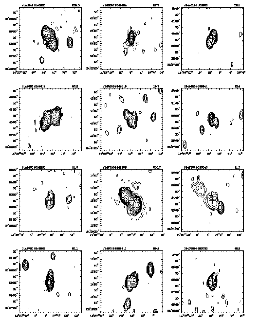
Figure 11: Plots of resolved sources with $S>10$ mJy. The contour levels are given by $(1+2^{n})\sigma$, with $n=1,2,...$ and $\sigma$ as the local background noise. Negative contours have the same spacing, and are plotted as dotted lines. The cross represents the nominal source center, and the object name and 1400 MHz flux densities are given in the upper left and right corners.

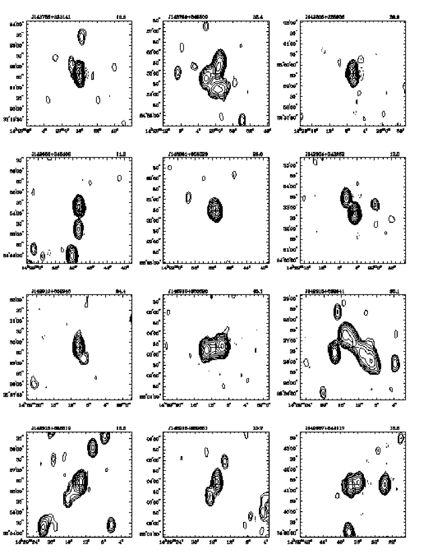
Figure 11: Continued

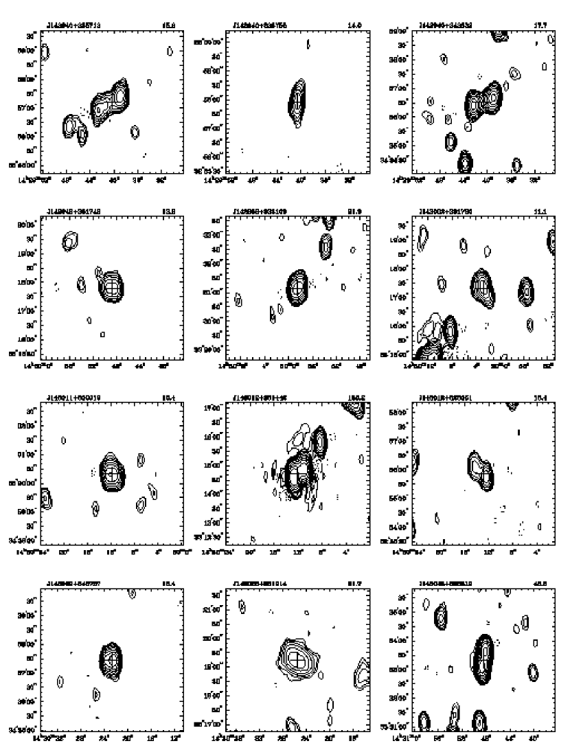
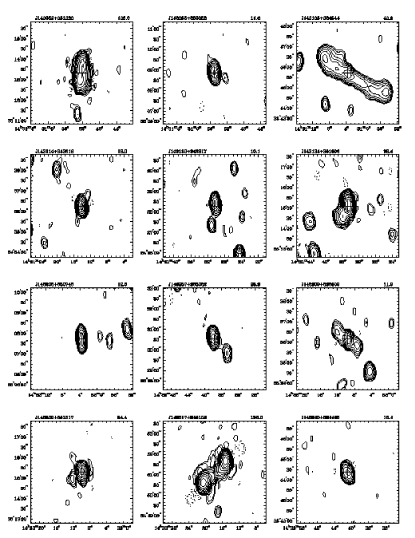
Figure 11: Continued

Figure 11: Continued

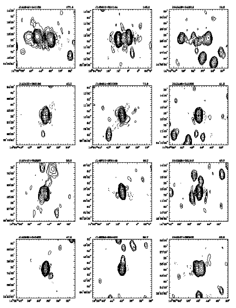
Figure 11: Continued

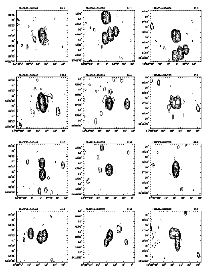
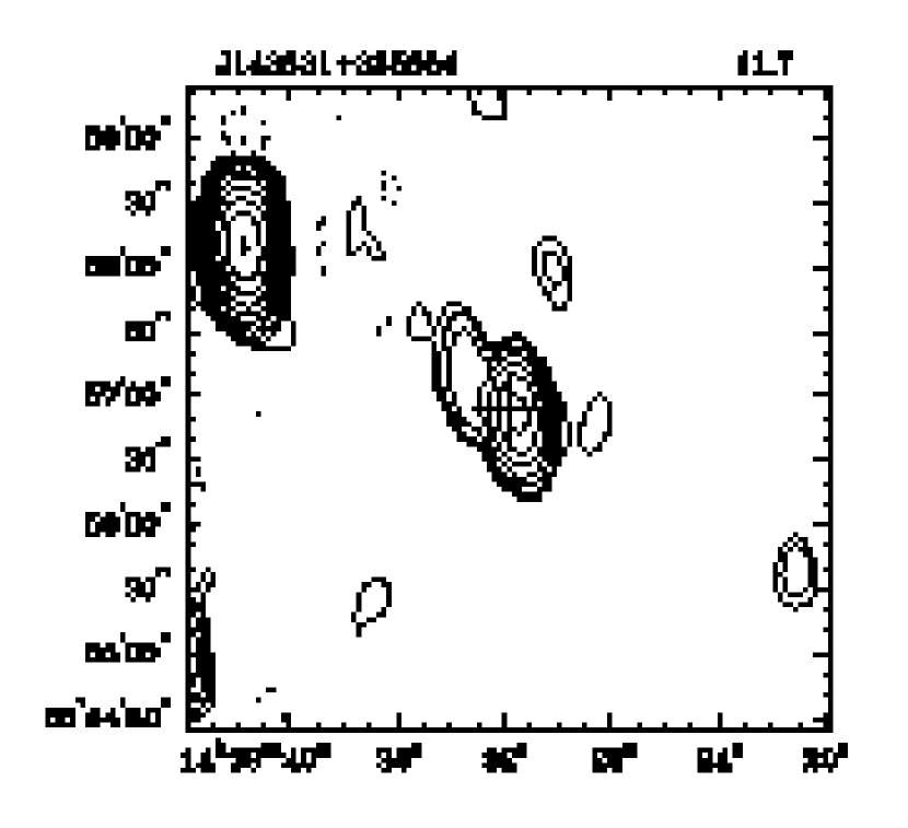
Figure 11: Continued

Figure 11: Continued

Table 1: Comparison between various radio surveys covering the Bootes field

Survey	Frequency	Resolution	Flux density limit	Detections in Bootes Field
WENSS	325	$54\arcsec\times 99\arcsec$	15	180
VLA-Bootes	325	$6\arcsec$	0.5	1200
NVSS	1400	$45\arcsec$	2.5	438
FIRST	1400	$5\arcsec$	1.0	749
WSRT-Bootes	1400	$13\arcsec\times 27\arcsec$	0.140	3172
87GB	4850	$222\arcsec\times 198\arcsec$	18	22

Table 2: Resolved sources with flux densities $>$10 mJy.

Source	RA (J2000)	Dec (J2000)	$\delta$POS	F	F${}_{\mbox{int}}$	rms	$\Theta\tablenotemark{c}_{\mbox{ma}}$	$\Theta\tablenotemark{c}_{\mbox{mi}}$	PA	LAS
			[$\arcsec$]		[mJy]	[mJy]	[$\arcsec$]	[$\arcsec$]	[$\arcdeg$]	[$\arcsec$]
J142541+345826	14 25 41.40	+34 58 26.6	0.4	M	$262.60\pm 10.5$	0.102	244	89	27	243
J142607+340424	14 26 07.73	+34 04 24.0	0.4	M	$37.73\pm 1.51$	0.048	111	49	164	108
J142610+333936	14 26 10.88	+33 39 36.6	0.4	M	$29.78\pm 1.19$	0.050	159	67	155	157
J142620+344012	14 26 20.94	+34 40 12.6	0.4	M	$87.01\pm 3.48$	0.034	231	77	130	229
J142639+344318	14 26 39.42	+34 43 18.6	0.4	M	$15.88\pm 0.64$	0.031	150	91	22	148
J142650+332941	14 26 50.53	+33 29 41.6	0.4	M	$13.41\pm 0.54$	0.038	103	60	22	99.4
J142656+352230	14 26 56.47	+35 22 30.9	0.4	M	$11.31\pm 0.46$	0.066	177	76	172	175
J142659+341159	14 26 59.96	+34 11 59.4	0.4	E	$305.74\pm 12.2$	0.042	229	81	48	227
J142702+333346	14 27 02.23	+33 33 46.1	0.4	E	$11.73\pm 0.47$	0.034	243	73	46	241
J142702+345905	14 27 02.24	+34 59 05.2	0.4	M	$21.14\pm 0.85$	0.031	150	56	179	148
J142716+331411	14 27 16.20	+33 14 11.5	0.4	M	$29.81\pm 1.19$	0.049	145	90	140	142
J142739+330750	14 27 39.33	+33 07 50.3	0.4	M	$43.62\pm 1.75$	0.049	128	71	161	125
J142756+332141	14 27 56.02	+33 21 41.3	0.4	M	$18.77\pm 0.75$	0.027	106	52	7	103
J142759+345500	14 27 59.82	+34 55 00.7	0.4	M	$32.37\pm 1.30$	0.026	178	94	167	176
J142806+325936	14 28 06.69	+32 59 36.7	0.4	M	$29.93\pm 1.20$	0.067	109	54	178	106
J142850+345408	14 28 50.51	+34 54 08.6	0.4	M	$11.18\pm 0.45$	0.024	180	36	178	178
J142851+353029	14 28 51.07	+35 30 29.5	0.4	M	$22.95\pm 0.92$	0.050	130	79	4	127
J142904+343252	14 29 04.89	+34 32 52.4	0.4	M	$12.98\pm 0.52$	0.018	142	43	24	139
J142910+352945	14 29 10.13	+35 29 45.1	0.4	M	$24.37\pm 0.98$	0.045	112	50	8	109
J142910+350320	14 29 10.88	+35 03 20.6	0.4	M	$43.10\pm 1.72$	0.025	159	80	108	157
J142913+332641	14 29 13.34	+33 26 41.3	0.4	M	$36.06\pm 1.44$	0.027	215	123	57	213
J142913+335619	14 29 13.51	+33 56 19.6	0.4	M	$18.51\pm 0.74$	0.027	172	76	151	170
J142915+330351	14 29 15.18	+33 03 51.4	0.4	M	$10.71\pm 0.43$	0.044	151	53	160	149
J142937+344117	14 29 37.07	+34 41 17.9	0.4	M	$15.33\pm 0.61$	0.022	104	76	131	100
J142940+335713	14 29 40.29	+33 57 13.0	0.4	M	$15.76\pm 0.63$	0.026	178	68	127	176
J142940+325755	14 29 40.48	+32 57 55.6	0.4	M	$14.04\pm 0.57$	0.071	162	58	175	160
J142940+343632	14 29 40.61	+34 36 32.0	0.4	M	$17.68\pm 0.71$	0.021	164	72	116	162
J142948+351748	14 29 48.72	+35 17 48.3	0.4	M	$13.18\pm 0.53$	0.031	125	97	25	122
J142958+333109	14 29 58.44	+33 31 09.6	0.4	M	$21.92\pm 0.88$	0.027	130	83	166	127
J143002+331720	14 30 02.68	+33 17 20.2	0.4	M	$11.07\pm 0.44$	0.032	141	79	17	138
J143011+350019	14 30 11.80	+35 00 19.4	0.4	M	$15.40\pm 0.62$	0.025	120	93	4	117
J143012+331442	14 30 12.02	+33 14 42.4	0.4	E	$185.15\pm 7.41$	0.034	142	61	148	139
J143012+325551	14 30 12.80	+32 55 51.6	0.4	M	$15.43\pm 0.63$	0.083	126	64	32	123
J143022+343727	14 30 22.68	+34 37 27.0	0.4	M	$16.44\pm 0.66$	0.023	99	74	3	95.2
J143025+351914	14 30 25.43	+35 19 14.6	0.4	M	$21.68\pm 0.87$	0.033	172	130	42	170
J143048+333319	14 30 48.35	+33 33 19.9	0.4	M	$46.61\pm 1.86$	0.027	183	54	171	181
J143052+331320	14 30 52.10	+33 13 20.5	0.4	M	$127.98\pm 5.12$	0.034	222	80	174	220
J143054+350852	14 30 54.99	+35 08 52.5	0.4	M	$11.61\pm 0.47$	0.028	104	59	10	100
J143103+334544	14 31 03.64	+33 45 44.1	0.4	E	$43.89\pm 1.76$	0.026	443	81	60	442
J143114+343616	14 31 14.08	+34 36 16.4	0.4	M	$18.03\pm 0.72$	0.023	109	50	175	106
J143130+342817	14 31 30.34	+34 28 17.9	0.4	M	$10.09\pm 0.40$	0.024	169	41	173	167
J143134+351506	14 31 34.68	+35 15 06.7	0.4	M	$98.43\pm 3.94$	0.033	130	58	165	127
J143203+330743	14 32 03.59	+33 07 43.7	0.4	M	$12.57\pm 0.51$	0.037	169	61	2	167
J143237+353032	14 32 37.63	+35 30 32.3	0.4	M	$28.30\pm 1.13$	0.056	136	54	32	133
J143309+333609	14 33 09.55	+33 36 09.8	0.4	M	$11.86\pm 0.48$	0.026	152	64	47	150
J143309+351517	14 33 09.92	+35 15 17.8	0.4	E	$34.40\pm 1.38$	0.033	102	68	175	98.4
J143317+345108	14 33 17.83	+34 51 08.1	0.4	E	$195.03\pm 7.80$	0.035	244	56	136	243
J143340+334423	14 33 40.88	+33 44 23.3	0.4	M	$15.39\pm 0.62$	0.029	128	80	17	125
J143341+341138	14 33 42.00	+34 11 38.1	0.4	E	$170.40\pm 6.82$	0.035	181	64	76	179
J143410+331144	14 34 10.42	+33 11 44.2	0.4	M	$144.96\pm 5.80$	0.039	142	67	101	139
J143429+342812	14 34 29.69	+34 28 12.2	0.4	E	$18.58\pm 0.74$	0.023	251	60	88	250
J143433+352136	14 34 33.20	+35 21 36.3	0.4	M	$39.99\pm 1.60$	0.040	113	67	167	110
J143434+351009	14 34 34.23	+35 10 09.6	0.4	M	$71.27\pm 2.85$	0.036	96	53	6	92.1
J143445+341220	14 34 45.20	+34 12 20.3	0.4	M	$41.91\pm 1.68$	0.028	104	61	5	100
J143445+332825	14 34 45.36	+33 28 25.8	0.4	M	$36.54\pm 1.46$	0.027	157	47	163	155
J143510+335445	14 35 10.11	+33 54 45.2	0.4	M	$40.66\pm 1.63$	0.034	110	55	5	107
J143528+331145	14 35 28.15	+33 11 45.5	0.4	M	$48.45\pm 1.94$	0.033	108	58	158	105
J143529+343423	14 35 29.15	+34 34 23.1	0.4	M	$47.94\pm 1.92$	0.024	99	54	3	95.2
J143539+344400	14 35 39.74	+34 44 00.7	0.4	M	$26.71\pm 1.07$	0.024	109	50	178	106
J143547+335536	14 35 47.78	+33 55 36.7	0.4	M	$53.21\pm 2.13$	0.034	99	93	62	95.2
J143553+352359	14 35 53.88	+35 23 59.8	0.4	M	$22.30\pm 0.89$	0.041	146	69	5	143
J143602+334353	14 36 02.94	+33 43 53.2	0.4	M	$11.15\pm 0.45$	0.030	210	92	127	208
J143604+334539	14 36 04.58	+33 45 39.5	0.4	M	$13.84\pm 0.56$	0.031	100	83	12	96.3
J143621+335949	14 36 21.94	+33 59 49.5	0.4	E	$127.08\pm 5.08$	0.037	163	64	5	161
J143623+352713	14 36 23.49	+35 27 13.7	0.4	M	$23.43\pm 0.94$	0.060	114	55	179	111
J143626+334703	14 36 26.19	+33 47 03.1	0.4	M	$10.13\pm 0.41$	0.030	140	112	117	137
J143703+343442	14 37 03.20	+34 34 42.0	0.4	M	$11.75\pm 0.47$	0.026	240	43	1	238
J143718+344653	14 37 18.98	+34 46 53.2	0.4	M	$11.76\pm 0.47$	0.030	126	85	2	123
J143739+343716	14 37 39.43	+34 37 16.5	0.4	M	$22.15\pm 0.89$	0.032	176	69	179	174
J143749+345452	14 37 49.78	+34 54 52.9	0.4	M	$41.87\pm 1.68$	0.045	132	89	133	129
J143814+342002	14 38 14.79	+34 20 02.0	0.4	M	$11.83\pm 0.48$	0.056	145	52	159	142
J143826+335023	14 38 26.37	+33 50 23.6	0.4	M	$15.66\pm 0.63$	0.056	235	103	15	233
J143831+335654	14 38 31.83	+33 56 54.5	0.4	M	$11.68\pm 0.47$	0.055	109	62	29	106

Table 3: Source Confusion Limits.

Lower flux limit	Expected Number of Objects within radius R
[mJy]	R = 30″	R = 60″	R = 120″
0.05	0.11	0.43	1.70
0.10	0.10	0.43	1.69
0.20	0.074	0.29	1.18
0.40	0.041	0.17	0.65
0.80	0.025	0.097	0.38
1.60	0.012	0.057	0.23
3.20	0.0083	0.036	0.14
6.40	0.0052	0.019	0.073
12.80	0.0026	0.0090	0.039
25.60	0.0012	0.0055	0.021
51.20	0.0007	0.0024	0.0095
102.40	0.0002	0.0005	0.0031
204.80	0.00002	0.0001	0.0007

Note. — The listed counts are the number of unrelated objects within a search radius R around a preselected target. For the total source count within a radius R, 1 should be added to this count therefore. The lower 2 flux density bins are affected by the incompleteness of the catalog at those levels; otherwise a factor of $\sim 2$ decrease in expected counts with increasing flux density threshold seems to be present. Also note the surface area factor of 4 in count levels between the columns. Objects within the 30″ radius are too close to be resolved by the WSRT beam, and would mistakenly be classified as a single source. To keep the number of significant digits approximately constant we had to increase the number of simulations with increasing flux density threshold.

Table 4: Catalog morphology break-down.

Morphology	Number	Density / sq.degree	Example object
Unresolved	2856	427.5
Barely resolved	43	6.4	J142851+353029
Double	136	20.4	J143703+343442
Triple	13	1.9	J143309+333609
Asymmetric	112	16.7	J143604+334539
Complex / Other	12	1.8	J143429+342812
Total	3172	474.9

Table 5: Sources with known redshifts.

Name	Alt. Name	RA (J2000)	DEC	ID	$z$	$V$	F1400
J142744+333829		14 27 44.49	+33 38 29.2	G	1.237	$\cdots$	14.18
J142823+331514	UGC 09284	14 28 23.42	+33 15 14.2	G: Sa?	0.01386	14.86	0.93
J142932+333038	CG 0447	14 29 32.66	+33 30 38.4	G	0.02638	17	0.12
J142934+352742	NGC 5646	14 29 34.07	+35 27 42.2	G: SBb	0.02861	14.99	1.37
J143025+351914	NGC 5656	14 30 25.43	+35 19 14.6	G: SAab	0.01051	12.73	15.33
J143119+343803	CG 0457	14 31 19.91	+34 38 03.9	G	0.01440	17.20	1.25
J143125+331349	CG 0459+0460	14 31 25.36	+33 13 49.9	G: S	0.02247	14.6	4.73
J143156+333830	VV 775	14 31 56.15	+33 38 30.1	G: Irr	0.03373	16	5.88
J143232+340626	LEDA 099838	14 32 32.42	+34 06 26.3	G	0.04264	17.96	0.21
J143518+350709	CG 0479	14 35 18.28	+35 07 09.2	G	0.02847	14.5	26.88

References

- Becker et al. (1995) Becker, R. H., White, R. L., & Helfand, D. J. 1995, ApJ, 450, 559
- Best et al. (1998) Best, P., Longair, M. S., & Röttgering, H. J. A. 1998,MNRAS, 295, 549
- Condon et al. (1998) Condon, J. J., Cotton, W. D., Greisen, E. W., Yin, Q. F., Perley, R. A., Taylor, G. B., & Broderick, J. J. 1998, AJ, 115, 1693
- De Breuck et al. (2000) De Breuck, C., van Breugel, W., Röttgering, H. J. A., & Miley, G. 2000, A&AS, 143, 303
- De Breuck et al. (2002) De Breuck, C., van Breugel, W., Stanford, A., Röttgering, H., Miley, G., & Stern, D. 2002, AJ, in press, astro-ph/0109540
- Dey et al. (1997) Dey, A., van Breugel, W., Vacca, W. D., & Antonucci, R. 1997, ApJ, 490, 698
- Dunlop & Peacock (1990) Dunlop, J., & Peacock, J. 1990, MNRAS, 247, 19
- Eales (1985) Eales, S. A. 1985, MNRAS, 217, 149
- Eales et al. (1997) Eales, S., Rawlings, S., Law-Green, D., Gotter, G., & Lacy, M. 1997, MNRAS, 291, 593
- Garrett et al. (2000) Garrett, M. A., de Bruyn, A. G., Giroletti, M., Baan, W. A., & Schilizzi, R. T. 2000, A&A, 361, L41
- Georgakakis et al. (1999) Georgakakis, A., Mobasher, B., Cram, L., Hopkins, A., Lidman, C., & Rowan-Robinson, M. 1999, MNRAS, 306, 708
- Gregory & Condon (1991) Gregory, P. C., & Condon, J. J. 1991, ApJS, 75, 1011
- Hopkins et al. (1998) Hopkins, A. M., Mobasher, B., Cram, L., & Rowan-Robinson, M. 1998, MNRAS, 296, 839
- Jarvis et al. (2001) Jarvis, M. J., Rawlings, S., Eales, S., Blundell, K. M., Bunker, A. J., Croft, S., McLure, R. J., & Willott, C. J. 2001, astro-ph/0106130
- Kaper et al. (1966) Kaper, H. G., Smiths, D. W., Schwartz, U., Takakubo, K., & van Woerden, H. 1966, Bull. Astron. Inst. Netherlands, 18, 465
- Katgert-Merkelijn et al. (1985) Katgert-Merkelijn, J., Robertson, J. G., Windhorst, R. A., & Katgert, P. 1985, A&AS, 61, 517
- Kauffmann & Haehnelt (2000) Kauffmann, G., & Haehnelt, M. 2000, MNRAS, 311, 576
- Kochanek et al. (2001) Kochanek, C. S., Pahre, M. A., Falco, E. E., Huchra, J. P., Mader, J., Jarrett, T. H., Chester, T., Cutri, R., & Schneider, S. E. 2001, astro-ph/0011456
- Kolkman (1993) Kolkman, O. M. 1993, The Westerbork Synthesis Radio Telescope User Documentation, NFRA
- (20) Laing, R. A., Riley, J. M., & Longair, M. S. 1983, MNRAS, 204, 151
- Laor (2000) Laor, A. 2000, ApJ, 543, L111
- Longair (1966) Longair, M. S. 1966, MNRAS, 133, 421
- McLure et al. (1999) McLure, R. J., Kukula, M. J., Dunlop, J. S., Baum, S. A., O’Dea, C. P., & Hughes, D. H. 1999, MNRAS, 308, 377
- Muxlow et al. (1999) Muxlow, T. W. B., Wilkinson, P. N., Richards, A. M. S., Kellermann, K. I., Richards, E. A., & Garrett, M. A. 1999, New Astronomy Review, 43, 623
- Oort (1987) Oort, M. J. A. 1987, A&AS, 71, 221
- Oort & Windhorst (1985) Oort, M. J. A., & Windhorst, R. A. 1985, A&A, 145, 405
- Owen & White (1991) Owen, F. N., & White, R. A. 1991, MNRAS, 249, 164
- Penterrici et al. (1999) Pentericci, L., Röttgering, H. J. A., Miley, G. K., McCarthy, P., Spinrad. H., van Breugel, W. J. M., & Macchetto, F. 1999, A&A, 341, 329
- Pentericci et al. (2000) Pentericci, L., Kurk, J. D., Röttgering, H. J. A., Miley, G. K., van Breugel, W., Carilli, C. L., Ford H., Heckman, T., McCarthy, P., & Moorwood, A. 2000, A&A, 361, L25
- Postman et al. (1998) Postman, M., Lauer, T. R., Szapudi, I., & Oegerle, W. 1998, in: “The Young Universe: Galaxy Formation and Evolution at Intermediate and High Redshift”, ASP Conference Series, Vol 146, eds. S. D’Odorico, A. Fontana, & E. Giallongo, p. 413
- Prandoni et al. (2000a) Prandoni, I., Gregorini, L., Parma, P., de Ruiter, H. R., Vettolani, G., Wieringa, M. H., & Ekers, R. D. 2000a, A&AS, 146, 31
- Prandoni et al. (2000b) Prandoni, I., Gregorini, L., Parma, P., de Ruiter, H. R., Vettolani, G., Wieringa, M. H., & Ekers, R. D. 2000b, A&AS, 146, 41
- Prandoni et al. (2001) Prandoni, I., Gregorini, L., Parma, P., de Ruiter, H. R., Vettolani, G., Zanichelli, A., Wieringa, M. H., & Ekers, R. D. 2001, A&A, 369, 787
- Rawlings, Eales & Lacy (2001) Rawlings, S., Eales, S., & Lacy, M. 2001, MNRAS, 322, 523
- Rengelink et al. (1997) Rengelink, R. B., Tang, Y., de Bruyn, A. G., Miley, G. K., Bremer, M. N., Röttgering, H. J. A., & Bremer, M. A. R. 1997, A&AS, 124, 259
- Richards et al. (1999) Richards, E. A., Fomalont, E. B., Kellermann, K. I., Windhorst, R. A., Partridge, R. B., Cowie, L. L., & Barger, A. J. 1999, ApJ, 526, L73
- Richards (2000) Richards, E. A. 2000, ApJ, 533, 611
- Sault et al. (1995) Sault, R. J., Teuben, P. J., & Wright, M. C. H. 1995, “A Retrospective View of Miriad”, in: Astronomical Data Analysis Software and Systems IV, ed. R.A. Shaw, H.E. Payne and J.J.E. Hayes. PASP Conf Series 77, 433 (1995).
- Sault & Conway (1999) Sault, R. J., & Conway, J. E. 1999, Synthesis Imaging in Radio Astronomy II, A Collection of Lectures from the Sixth NRAO/NMIMT Synthesis Imaging Summer School, ASP Conference Series, Vol 180, eds. G. B. Taylor, C. L. Carilli, & R. A. Perley, p. 21
- White & Becker (1992) White, R. L., & Becker, R. H. 1992, ApJS, 79, 331
- Windhorst et al. (1999) Windhorst, R. A., Hopkins, A., Richards, E. A., & Waddington, I. 1999, in “The Hy Redshift Universe”, ASP Conference Series, Vol 193, eds. A. J. Bunker & W. J. M. van Breugel, p. 55
- Wall (1994) Wall, J. V. 1994, Australian Journal of Physics, 47, 625