[

Have Acoustic Oscillations been Detected in the Current Cosmic Microwave Background Data?

Abstract

The angular power spectrum of the Cosmic Microwave Background has been measured out to sufficiently small angular scale to encompass a few acoustic oscillations. We use a phenomenological fit to the angular power spectrum to quantify the statistical significance of these oscillations and discuss the cosmological implications of such a finding.

] During the past few years there has been unprecedented progress in the detection and characterization of fluctuations in the Cosmic Microwave Background on small angular scales. The TOCO, BOOMERanG and MAXIMA experiments [1] presented unambiguous evidence for a preferred scale (a “peak”) in the variance of temperature fluctuations as a function of scale, $(\Delta T)^{2}_{\ell}\equiv\ell(\ell+1)C_{\ell}/4\pi$ (where $C_{\ell}$ is the angular power spectrum at a scale $\ell\simeq 180^{\rm 0}/\theta$). This is a striking result, having been predicted in 1970 from simple assumptions about scale-invariance and linear perturbation theory of General Relativity. During the last six months the possible presence of peaks and troughs in $(\Delta T)^{2}_{\ell}$ has been reported by the BOOMERanG [2], DASI [3] and MAXIMA [4] experiments. This harmonic set of features in the power spectrum could further confirm that the origin of structure was due to a primordial set of fluctuations which set the cosmological plasma “ringing” at very early times. It is the purpose of this short note to quantify the confidence with which one can claim that there are acoustic oscillations present in the current data.

We shall first outline the argument for why we expect oscillations in the power spectrum of the CMB. Let us restrict ourselves to the radiation era, where the photons and baryons are tightly coupled. Its suffices to consider the density contrast in radiation, $\delta_{\gamma}$ and (in the synchronous gauge) the trace of the spatial metric perturbations $h\equiv h^{i}_{i}$. The first order Einstein and continuity equations in Fourier space are:

$${\ddot{h}}+\frac{1}{\eta}{\dot{h}}+\frac{6}{\eta^{2}}\delta_{\gamma}=0\ \ \mbox{\rm and}\ \ {\ddot{\delta}_{\gamma}}+\frac{k^{2}}{3}\delta_{\gamma}+\frac{2}{3}{\ddot{h}}=0$$ (1)

where $\eta$ is conformal time and $k$ labels the Fourier component. Let us restrict ourselves to adiabatic initial conditions. In this case one has that $\delta_{\gamma}=-\frac{2}{3}h$. One can solve Eq. 1 on large scales $k\eta\ll 1$ to find two solutions $\delta_{\gamma}=A_{\bf k}\eta^{2},B_{\bf k}\eta^{-2}$; if these are setup early in the radiation era, the growing dominates very rapidly and one can to as excellent approximation set $B_{\bf k}=0$. On small scales one can solve the system using a WKB approximation to find $\delta_{\gamma}\propto\cos(k\eta/\sqrt{3}),\sin(k\eta/\sqrt{3})$. Matching the large scale solution to the small scale solution one finds that $\delta_{\gamma}=A_{\bf k}(k\eta)^{2}\cos(k\eta/\sqrt{3}+\phi)$. The acoustic oscillations in the $\Delta T^{2}_{\ell}$ will be primarily the power spectrum of $\delta_{\gamma}$ at recombination, $\eta_{*}$ projected until today:

$$\Delta T^{2}_{\ell}\propto\langle|A_{\bf k}|^{2}\rangle\cos^{2}(\frac{k\eta_{*}}{\sqrt{3}}+\phi)\mid_{\ell=k\chi(\eta_{0}-\eta_{*})}$$ (2)

where $\chi(r)$ is the conformal distance corresponding to the coordinate distance $r$. Thus, the oscillations in the baryon-photon plasma will lead to a set of peaks and troughs in the angular power spectrum.

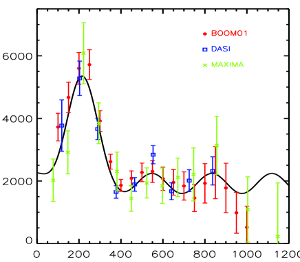
FIG. 1.: Data from BOOMERANG, DASI and MAXIMA. Overplotted, our best fit from the class of models described by Eq. 3.

How general is this argument? As stated above we are considering primordial, passive, perturbations which are in effect initial conditions for the evolution of the coupled baryon/photon plasma responding to gravity and pressure [5]. The most general class of such perturbations was classified in [6] where, in the context of the current menagerie of matter candidates, it is believed that there are five degrees of freedom, possibly correlated among each other (corresponding to a $5\times 5$ symmetric matrix of initial conditions). Although we looked at the specific case of adiabatic perturbations, the argument follows through for all other pure primordial perturbations. By pure perturbations we means perturbations in which one only picks one of these degrees of freedom to be non-zero. The key feature is that the large scale solutions to Eq. 1 have two modes, one of which is decaying and very rapidly becomes subdominant. For example for density isocurvature perturbations a different phase, $\phi$ will be picked out such that the positions of the peaks will be out of phase with regards to the adiabatic models. If one considers sums of initial condition such as in [6], then it is conceivable that the combination of power spectra will interfere in such a way as washout the oscillations.

Clearly, the presence of oscillatory features would be strong evidence that the structure was seeded at some early time, before recombination. With the current CMB data it has been suggested that we are already seeing evidence for such features. One of the reasons for such a claim is that primordial, passive models supply a good fit to the measured angular power spectrum and, as argued above these models have acoustic oscillations. The concern is that, all models which have been compared to the data have oscillations in the $C_{\ell}$ and one therefore has not strictly tested for the presence of these oscillations. We propose to do this in the following: construct a phenomenological fit to the data points that can smoothly interpolate between a model with no oscillations to one which has oscillations of a well defined frequency and phase. An analogous approach was used in [7] to quantify the significance of the presence of a peak at $\ell\simeq 200$. The parametrization we shall use is of the following form:

$$\Delta T^{2}_{\ell}=Ae^{-\frac{(\ell-\ell_{p})^{2}}{2\sigma^{2}}}+B\cos^{2}[\alpha(\ell-\ell_{p})+\phi]+C$$ (3)

This is a seven parameter family of models and we can justify it as follows. The goal is to detect the presence of prefered frequency in the $\Delta T^{2}_{\ell}$ so the parameters we are ultimately interested in are $\alpha$ and $B$. However we know that there is a well defined peak in the data with a well defined width, and the signal to noise of this peak is sufficiently high that it will dominate any statistical analysis; i.e. the width of the peak, $\sigma$ will tend to peak at a frequency of order $\pi/\sigma$. Given that we wish to be conservative we consider a part of the curve corresponding to the first peak (characterized by $A$, $\ell_{p}$ and $\sigma$) and marginalize over these parameters. Hopefully in this way we decrease the statistical weight of the peak. Finally we introduce an offset, $C$ which allows us to interpolate between a flat and oscillatory curve.

Given that we are interested in the behaviour of the power spectrum in the regime where acoustic oscillations will dominate, i.e. on scales larger than the sound horizon at last scattering, we shall not include the COBE data set. We restrict ourselves to three data sets, BOOMERanG [2], DASI [3] and MAXIMA [4]. We shall minimize the fitting function of Eq. 3 with regards to the three data sets using a standard $\chi^{2}$. A few comments are in order. We do not consider more refined parametrizations of the band-power distribution functions[8], such as the off-set log-normal or the skewed approximation. We marginalize over the calibration uncertainties quoted in [2, 3, 4]. Furthermore the beam uncertainties are taken into account by adding them in quadrature to the noise covariance matrices of each experiment. All these approximations may introduce a modest degree of uncertainty in our results but do not change the essential conclusions.

Experiment	$\alpha\times 10^{-2}$	$B\times 10^{3}$ ($\mu$K)2	$\chi^{2}$ ($N_{D}$)
All	$1.1^{+0.2}_{-0.4}$	$0.7^{+0.3}_{-0.3}$	$30$ ($42$)
All>400	$1.0^{+0.3}_{-0.6}$	$0.8^{+0.3}_{-0.3}$	$16$ ($27$)
BOOMERanG	$0.8^{+0.6}_{-0.7}$	$0.7^{+0.4}_{-0.4}$	$6$ ($19$)
MAXIMA	$0.7^{+0.8}_{-0.6}$	$1.0^{+1.0}_{-0.9}$	$3$ ($14$)
DASI	$1.1^{+0.3}_{-0.3}$	$1.1^{+0.4}_{-0.5}$	$2$ ($9$)
DASI-1	$0.9^{+0.6}_{-0.8}$	$0.9^{+1.0}_{-0.7}$	$1$ ($8$)
MOCK	$1.0^{+0.3}_{-0.3}$	$0.7^{+0.3}_{-0.3}$	$34$ ($42$)
MOCK>400	$1.0^{+0.3}_{-0.3}$	$0.6^{+0.3}_{-0.3}$	$27$ ($27$)

TABLE I.: The mean values and 95% errors for the $\alpha$ and $B$ as defined in Equation 3 and the corresponding $\chi^{2}$ for the best fit models (where $N_{D}$ is the number of parameters). See text for description of the different data combinations.

In table I we summarize our results for $\alpha$, $B$ and the $\chi^{2}$ of the best fit model to each subset of data. The different combination and subsets of the data we consider are: data from all three experiments (“All”) and for all three data experiments discarding all points with $\ell<400$ (“All_>400”), the data from each individual experiment (“BOOMERanG”, “MAXIMA” and “DASI”), data from DASI discarding the point at $\ell=553$ (“DASI_-1”). We have also generated a mock realization of the best fit adiabatic model to the data with corresponding variance from sampling and noise from the combination of the three experiments (“Mock”) and finally the same realization but discarding all points with $\ell<400$ (“Mock_>400”). We present the mean values and the $95\%$ confidence limits from the integrated likelihoods. We find that the data does seem to pick out a favorite frequency of oscillation in the $\Delta T^{2}_{\ell}$ of $\alpha=1.1^{0.2}_{-0.1}$, corresponding to an interpeak spacing of $\delta\ell=\pi/\alpha=286^{+163}_{-44}$. It is interesting to note that even removing the points that lie in the region of the 1^st peak, the detection persists albeit with larger error bars. The three experiments detect similar values of $\alpha$ with varying confidence regions. We should note that the likelihoods in $\alpha$ are extremely skewed and in some cases actually have two local maxima. For example the maximum of the likelihood for BOOMERanG is $\alpha=0.01$ while for MAXIMA there is a local maximum at $\alpha=0.011$. Note also the importance of the point at $\ell=553$ in the DASI data. If we remove this point from our analysis, the DASI confidence region for $\alpha$ enlarges considerably. We have listed the values of the $\chi^{2}$ for the corresponding best fit models along with the number of data points used in each case. All of the $\chi^{2}$ are reasonable although correlations between the data points may lead to a smaller number of degrees of freedom than simply $N_{D}-N_{P}$ where $N_{P}=6$ is the number of parameters. The Mock data sets lead to similar values of $\alpha$ and corresponding confidence limits.

Our analysis indicates that there is a marginal presence of oscillations in the measured $\Delta T^{2}_{\ell}$ (at the $2-\sigma$ level) within the context of the phenomenological model described by Eq. 3. This caveat is important. Although we have attempted to justify the functional form of our model using rough general arguments, it is conceivable that one could construct other models which interpolate between oscillatory and non-oscillatory behaviour and which reduce or enhance the significance of detection of $\alpha$. For example, if we consider the All_>400 combination of data and add a term of the form $D\ell$ to Equation 3., the mean value of $\alpha$ is still $0.01$ but now $\alpha=0$ lies within the $95\%$ confidence region. We have, of course, done this by adding yet another parameter. However this does not exclude the possibility that there are models with fewer parameters and no oscillations that may provide a better fit to the data.

Let us pursue the implications of the constrain on $\alpha$ within the context of models which predict oscillations. The above discussion leads us to note that the spacing between peaks $\delta\ell$ can be used to set a constraint on the angular-diameter distance. As noted in [9] the physical peak separation is set by the sound-horizon (which we know from atomic physics). Combined with the our knowledge of time of recombination and $\delta\ell$ (which is effectively half the angular scale subtended by the sound horizon at recombination) we can constrain the geometry of the universe. Efstathiou and Bond [10] have proposed a convenient parametrization using the “shift” parameter $R=2\sqrt{\Omega_{K}/\Omega_{M}}/\chi(\eta_{0}-\eta_{*})$ where $\Omega_{K}=1-\Omega_{\Lambda}-\Omega_{M}$ and $\Omega_{M}$ ($\Omega_{\Lambda}$) are the fractional energy densities of matter (cosmological constant) today. Indeed one has that $\delta\ell\simeq 290/R$ and one can obtain a likelihood for $R$: one finds that $R=1.01^{+0.18}_{-0.37}$. This can be reexpressed into a constrain on $\Omega=1-\Omega_{K}$ if we marginalize over $\Omega_{\Lambda}$ to obtain $\Omega\simeq 1^{+0.24}_{-0.18}$. Note that this constraint is independent from the constraint obtained from the assumption of adiabaticity and the position of the first peak, $\ell_{p}\simeq 215/R$ where one finds $R=1.05^{+0.05}_{-0.04}$ and $\Omega\simeq 1^{+0.2}_{-0.12}$. These two independent constraints on $R$ and $\Omega$ are consistent.

In summary we have attempted to assess the significance of the presence of acoustic oscillations in current CMB data using a model independent method. One could view Eq. 3 as a different class of phenomenological models which has the advantage (given the question we are attempting to answer) of smoothly interpolating between the absence and presence of acoustic oscillations. We subsequently use the interpeak separation (or acoustic oscillation frequency) to derive a constraint on the geometry of the universe. Such a constraint is independent to that derived from the position of the first peak. However it is necessarily included in any analysis which considers the full set of initial conditions put forward in [6]. With the rapid progress of CMB experiments, such an analysis will become essential to obtain accurate, model independent constraints on the cosmological parameters.

Acknowledgments: PGF acknowledges support from the Royal Society. The authors thank F. Vernizzi, M. Kunz, A. Melchiorri and the MAXIMA collaboration for discussions and advice.

REFERENCES

- [1] A.D.Miller et al Ap. J. 54, L1 (1999); P. de Bernardis et al Nature, 404, 955 (2000); S. Hanany et al Ap. J. 545 L5 (2000);
- [2] C.B.Netterfield et al astro-ph/0104460 (2001);
- [3] C.Pryke et al astro-ph/0104490 (2001);
- [4] A.T.Lee et al astro-ph/0104459 (2001);
- [5] A.Albrecht, D. Coulson, P.G. Ferreira & J. Magueijo PRL 76 1413 (1996); J. Magueijo, A.Albrecht, D.Coulson & P.G.Ferreira PRL 76 2617 (1996);
- [6] M.Bucher, K.Moodley & N.Turok astro-ph/0007360 (2000);
- [7] L.Knox & L.Page PRL, 85, 1366 (2000);
- [8] J.R.Bond, A.H.Jaffe & L.Knox PRD, 57, 2117 (1998); J.Bartlett, M.Douspis, A.Blanchard & M. Le Dour A&AS, 146, 507 (2000);
- [9] W.Hu & M.White Ap.J. 771, 30 (1996);
- [10] G.Efstathiou & J.R.Bond MNRAS, 304, 75 (1999); A.Melchiorri & L.M.Griffiths, New Ast. Rev, 45, 321 (2001).