Accurate Stellar Population Studies
from Multiband Photometric Observations^†

Abstract

We present a new technique based on multi-band near ultraviolet and optical photometry to measure both the stellar intrinsic properties, i.e. luminosity and effective temperature, and the interstellar dust extinction along the line of sight to hundreds of stars per square arcminute. The yield is twofold. On the one hand, the resulting reddening map has a very high spatial resolution, of the order of a few arcseconds, and can be quite effectively used in regions where the interstellar material is patchy, thus producing considerable differential extinction on small angular scales. On the other hand, combining the photometric information over a wide baseline in wavelength provides an accurate determination of temperature and luminosity for thousands of stars. As a test case, we present the results for the region around Supernova 1987A in the Large Magellanic Cloud imaged with the WFPC2 on board the Hubble Space Telescope.

1 Introduction

Stars provide most of the light we detect in the Universe and the entire chemical and dynamical evolution of galaxies is strongly influenced by the formation of many generations of stars. The most massive ones enrich the surrounding medium of highly processed material and supply vast amounts of kinetic energy (both with their winds and, even more, with their ultimate explosions as Type II Supernovæ). Lower mass stars constitute one of the main sources of crucial elements, such as Carbon and Nitrogen (through stellar winds first, and planetary nebula ejection later) in their individual evolution, and may be the main suppliers of the iron group elements if, in binary systems, they succeed to merge and explode as Type Ia Supernovæ.

A major problem that one encounters almost ubiquitously when studying stars is the effect that interstellar dust has on the observed spectral distribution of their light. A precise measurement of the interstellar reddening along the line of sight to the stars under study is the first step, and a crucial one, towards determining the intrinsic properties of the stellar populations. All sky reddening maps, such as the one derived from dust temperature by Schlegel et al (1998), for example, may not be satisfactory for detailed stellar populations studies. For example, it cannot be used in the direction of nearby galaxies, such as the Magellanic Clouds and M31. Also, the derived value of the dust column density is extremely sensitive to dust temperature and, in any case, not accurate for high values of extinction ($A_{V}>0.5$ mag, Arce & Goodman, 1999). Moreover, the angular resolution of the map is pretty coarse ($\sim 6^{\prime}$, as compared to a few arcseconds for the method presented here) and, thus, it does not allow to cope effectively with the patchy structure typical of the interstellar medium.

It is certainly preferable to determine the amount of dust in front of the stars from the light coming from the stars themselves. While spectroscopic data may certainly provide an accurate determination of the reddening and the stellar parameters, the multiplexing capabilities of current spectrographs are limited, at best, to a few tens of (relatively bright) objects per telescope pointing. The method we describe in this paper overcomes this limitation by using only imaging and, thus, providing measurements of both the stellar parameters and the reddening along the line of sight to thousands of stars per pointing. The gain in terms of statistics is obviously tremendous. As a consequence, the spatial resolution of the resulting extinction map is extremely high, with an $E(\mathrm{B}-\mathrm{V})$ measurement every few arcseconds, even for moderately dense star fields. While here we test this newly developed technique on HST-WFPC2 observations, the method can be applied to data obtained with any instrument. The quality of the final result, however, will obviously depend on the quality of the input photometry.

The whole purpose of this paper is to describe a method to retrieve the stellar parameters from this kind of data by fitting model atmospheres to the observed fluxes. In section 2 we describe the dataset considered and the reduction techniques adopted. In section 3 the limitations of the classical approach based on Color-Magnitude diagrams are discussed and the method we have developed to overcome them via a multiband fit to the observed spectra is presented in section 4. The results of this procedure are discussed in section 5, while section 6 deals with the effects that the gravity and metallicity of the input model spectra have on the derived parameters. Finally, the spectral coverage needed to recover bot $\mathrm{T}_{eff}$ and $E(\mathrm{B}-\mathrm{V})$ is explored in section 7 and the role of random and systematic errors is assessed in section 8.

The broad band colors in selected WFPC2 filters and the corresponding extinction coefficients, which are needed for any application of our procedure, are provided in appendix AppendixB: Broad band colors and extinction coefficients in selected WFPC2 filters.

2 Observations and Data Reduction

Our method was developed and tested using HST-WFPC2 multiband observations. In particular, we have taken advantage of the wealth of information provided by the repeated observations of Supernova 1987A (SN1987A) and the field surrounding it in the Large Magellanic Cloud (LMC). Since 1994, Supernova 1987A was imaged with the WFPC2 every year as a part of the Supernova INtensive Study project (SINS, PI: Robert P. Kirshner). The log of the observations we have used is reported in Table 1. The WFPC2 filters do not exactly match any of the ground-based photometric systems and the closest analog of the passbands we have used is reported in the last column of this Table. The observations cover an almost circular portion of the sky centered on SN1987A and with a radius of $130^{\prime\prime}$, corresponding to roughly 32 pc at the distance of the LMC (51.4 kpc, Panagia, 1999; Romaniello et al, 2000). The true color image derived from our data is shown in Figure Accurate Stellar Population Studies from Multiband Photometric Observations^†.

The observations were processed through the standard PODPS (Post Observation Data Processing System) pipeline for bias removal and flat fielding. In all the cases the available images for each filter were combined to remove cosmic rays events. The long baseline in wavelength that they cover (more than a factor of 4, extending from $\sim$2,300 to $\sim$9,600 Å) together with the unprecedented spatial resolution of WFPC2 ($\sim 0^{\prime\prime}.1$, i.e. roughly 0.03 pc at the distance of the LMC) make of this dataset a unique and ideal one to investigate the problem of disentangling the effects of reddening from those of different effective temperatures for stars of different spectral type.

The plate scale of the camera is 0.045 and 0.099 arcsec/pixel in the PC and in the three WF chips, respectively. We performed aperture photometry following the prescriptions by Gilmozzi (1990) as refined by Romaniello (1998), i.e. measuring the flux in a circular aperture of 2 pixels radius and the sky background value in an annulus of internal radius 3 pixels and width 2 pixels. Aperture photometry is perfectly adequate for our study because crowding is never a problem in our images. Actually, the average separation of stars from each other is about 1.3^′′ (i.e. $\sim 29$ pixels in the PC chip and $\sim 13$ pixels in the WF ones) which is much larger than the WFPC2 PSF width. We have used the IRAF-synphot synthetic photometry package to compute the theoretical Data Numbers to be compared to the observed ones. The WFPC2 calibration and, consequently, the synphot results are typically accurate to within $\pm$ 5% (Whitmore, 1995; Bagget et al, 1997).

We identify the stars in the deepest frame (F555W, i.e. V band-like filter) and then measure their magnitudes in all of the other filters. The total number of stars identified in this way is 21,955. If a star is not detected in a band, then its magnitude in that band is substituted by a $3\sigma$ upper limit. For about 12,340 of them, i.e. 56%, the photometric accuracy is better than 0.1 mag in the F555W, F675W and F814W filters. The number of stars with accuracy better than 0.1 mag drops to 6,825 (31%) in the F439W band, and only 786 (3.6%) stars have an uncertainty in the F255W filter smaller than 0.2 mag.

The brightest stars in each CCD chip are saturated (i.e. most stars brighter than 17.5 in the F555W passband). We recover their photometry either by fitting the unsaturated wings of the PSF for moderately saturated stars, i.e. with no saturation outside the central 2 pixel radius, or by following the method developed by Gilliland (1994) for heavily saturated stars. In most cases, the achieved photometric accuracy is better than 0.05 magnitudes. Full description of the methods used can be found in Romaniello (1998). As a sanity check we have compared our photometry in the F439W and F555W bands with ground-based one in B and V (28 stars brighter than $V\simeq 20$ within 30^′′ from SN1987A, Walker & Suntzeff, 1990) and found an overall excellent agreement, i.e. rms deviations less than 0.05 mag in both filters, except for the obvious cases of few stars that appear as point-like in ground based images but are resolved into more than one object on the WFPC2 frames. This result confirms the accuracy of our photometric measurements and the quality of the WFPC2 calibration.

We shall see in section 4 that a good photometric quality in different bands is needed in order to recover $E(\mathrm{B}-\mathrm{V})$ and stellar temperature. In order to select stars with a good overall photometry we define the mean error in 5 bands ($\overline{\delta}_{5}$) (i.e. excluding the UV F255W band) as:

$$\overline{\delta}_{5}=\sqrt{\frac{\delta_{\mathrm{F336W}}^{2}+\delta_{\mathrm{F439W}}^{2}+\delta_{\mathrm{F555W}}^{2}+\delta_{\mathrm{F675W}}^{2}+\delta_{\mathrm{F814W}}^{2}}{5}}$$ (1)

In addition to the main field described above, we have also used a second set of WFPC2 images pointing $8^{\prime}$ south-east of SN1987A. As shown in Table 2 in this case we only use 4 filters and the F336W and F439W passbands are substituted with their broader counterparts F300W and F450W, respectively. Being broader, the latter are more efficient and allowed us to save precious telescope time, always a crucial issue, without losing any vital information (see section 7).

3 Color-Magnitude diagrams

As it can be seen in Figure Accurate Stellar Population Studies from Multiband Photometric Observations^† Supernova 1987A and its rings are right at the center of the field imaged with WFPC2 and belong to a loose cluster of blue stars (see Panagia et al, 2000). Also, the interstellar medium, as traced by the $\mathrm{H}\alpha$ emission coded in red in Figure Accurate Stellar Population Studies from Multiband Photometric Observations^†, is far from being spatially uniform and its distribution varies on scales of few arcseconds (let us recall here that 1^′′ corresponds to roughly 0.25 pc at the distance of the LMC). Since the spatial distribution of dust usually follows the one of gas (see, for example, Mathis, 1990), one can expect the interstellar reddening to vary on similar, if not even smaller, scales. This is further confirmed by an inspection of Figure Accurate Stellar Population Studies from Multiband Photometric Observations^† where we show the Color-Magnitude diagrams (CMD) for different combination of bands.

The black dots in each CMD in Figure Accurate Stellar Population Studies from Multiband Photometric Observations^† are the 6,695 stars with $\overline{\delta}_{5}<0.1$ mag, where $\overline{\delta}_{5}$ is the mean error defined in equation (1). The error threshold of $\overline{\delta}_{5}<0.1$ reflects itself as a magnitude threshold at $m_{\mathrm{F555W}}\simeq~{}23$. We estimate that the completeness at this magnitude limit is very close to 100% because the density of detected stars down to 23th magnitude is rather low, i.e. about 1 star per 4.6 square-arcsec area (Panagia et al, 2000).

It is apparent that, despite the high quality of the measurements (internal uncertainties less than 0.1 magnitudes, see also Figure Accurate Stellar Population Studies from Multiband Photometric Observations^†), the various features of the CMDs, such as the Zero Age Main Sequence for the early type stars and the Red Giant clump for the more evolved populations, are rather “fuzzy” and not sharply defined. Although this is due in part to the presence of several stellar populations projected on each other (Panagia et al, 2000), most of the problem arises from the fact that reddening is not quite uniform over the field, thus causing the points of otherwise identical stars to fall in appreciably different locations of the CMDs.

4 The fitting procedure

The large number of bands available in our dataset provides a sort of wide-band spectroscopy which defines the continuum spectral distribution of each star quite well. Of course, the resolution is very low, of the order of $\lambda/\Delta\lambda\simeq~{}7$, but, still, important features, such as the Balmer jump between the HST  F336W and F439W bands, are clearly visible. Four examples of “wide band spectra” are shown in Figure 1 (the flux F_λ is expressed in units of erg cm^-2 s^-1 Å^-1) and their observed magnitudes are listed in Table 3. The whole purpose of this paper is to describe a method to retrieve the stellar parameters from this kind of data by fitting model atmospheres to the observed fluxes.

The shape of the observed spectrum is mostly determined by the effective temperature of the star and by the amount of dust along the line of sight. The other quantity of interest, namely the solid angle subtended by the star (or, correspondingly, its angular radius) is obtained by a straight normalization of the spectral distribution.

The general idea of our method is to recover simultaneously the extinction along the line of sight and the effective temperature of a star by fitting the observed magnitudes to the ones computed using stellar atmosphere models reddened by various amounts of $E(\mathrm{B}-\mathrm{V})$. The angular radius, then, is directly obtained from the ratio of the observed flux, dereddened with the best fitting $E(\mathrm{B}-\mathrm{V})$ value, to the one at the surface of the star, as given by the best fitting model atmosphere. Thus, the two fundamental ingredients that go into the fit are the stellar atmosphere models and the reddening law: we have adopted the models by Bessel et al (1998) and the reddening law by Scuderi et al (1996).

We have chosen the models by Bessel et al (1998), as they provide a well tested, homogeneous set covering the temperature interval between 3,500 and 50,000 K in the wavelength range between 90 Å  and 160 $\mu m$. They are computed with an updated version of the ATLAS9 code used for the Kurucz (1993) models with no allowance for convective overshooting, as discussed by Castelli et al (1997a, b).

We have used the IRAF task synphot to compute the theoretical magnitudes at the surface of the star for the grid of temperatures provided by Bessel et al (1998) by convolving the model spectra with the HST+WFPC2 response curves. Once the convolution is performed, we use a spline interpolation to get a temperature grid with a logarithmic step of 0.005, i.e. 1%. We have used model atmospheres with $\log(g)=4.5$ (cgs units), which is the typical value for Main Sequence stars, and Z$=0.3\cdot$Z_☉, the mean expected metallicity of the LMC. In section 6 we will analyze and discuss the effects of these two parameters on the fit and we will see that neither of them affects the values of the derived parameters appreciably.

In order to faithfully model the data, we have computed separately the expected counts that a given spectrum produces on each of the four WFPC2 chip detectors. Also, the throughput variation between decontaminations of the camera (Bagget et al, 1996) was taken into account by specifying the Julian date of the observation (the cont keyword in synphot). Details of this procedure can be found in Romaniello (1998), while model magnitudes for solar and one third solar metallicity are listed here in Tables (6) and (7), respectively.

The other input ingredient is the reddening law. This is a combination of foreground extinction due to dust in the Milky Way and internal extinction in the LMC. We have taken the first component to be the same for all of the stars, with ${E(\mathrm{B}-\mathrm{V})}_{\mathrm{MW}}=0.05$ (see, for example, Schwering & Israel, 1991) and we have used the Galactic reddening law as compiled by Savage & Mathis (1979). On the other hand, the amount of extinction from the LMC dust is one of the parameters of the fit. We have taken the LMC reddening law in the direction of our field to be the one determined by Scuderi et al (1996) from a study of an HST-FOS ultraviolet and optical spectrum of Star 2, one of the companions to SN1987A projected just 3^′′.9 NW of it. It is, of course, crucially important to use a reddening law derived in the same field under study, as it may vary considerably from place to place on quite small angular scales (see, for example, Whittet, 1992). These reddening laws were used to compute the extinction coefficients in the WFPC2 passbands for every combination of input model spectrum and value of $E(\mathrm{B}-\mathrm{V})$ (see Table 8).

The fitting procedure consists of two steps:

• we first use a reddening-free color to determine which stars can be used to measure the reddening unambiguously;

• once this is done, we use the full information from the 6 bands to fit the observed spectral energy distribution for all of the stars.

We will now describe these two steps.

4.1 First step: reddening-free colors

It is a well known fact that the solution in the $E(\mathrm{B}-\mathrm{V})$-$\mathrm{T}_{eff}$ plane may not be unique for stars later than, roughly speaking, A0 and that different combinations of temperature and reddening may lead to almost indistinguishable optical and near-UV low resolution spectra. An example is shown in Figure 2 where we compare Bessel et al (1998) models for three combinations of temperature and reddening: $\mathrm{T}_{eff}=5,000$ K and ${E(\mathrm{B}-\mathrm{V})}=0$ (short-dash line), $\mathrm{T}_{eff}=7,600$ K reddened by ${E(\mathrm{B}-\mathrm{V})}=0.55$ (long-dash line) and, finally, $\mathrm{T}_{eff}=12,000$ K and ${E(\mathrm{B}-\mathrm{V})}=0.86$ (full line). The spectra are normalized to the F814W flux and errorbars corresponding to 0.1 mag are shown. To all practical purposes the spectra are identical for wavelengths longer than 3,300 Å and only good data in the ultraviolet can help to distinguish them. Unfortunately, though, these data are often not available, as imaging in the ultraviolet can only be done from space and it requires very long exposure times for red stars . The purpose of first step of the procedure, then, is to use a reddening-free color to eliminate the $E(\mathrm{B}-\mathrm{V})$-$\mathrm{T}_{eff}$ degeneracy when no ultraviolet observations are available.

Let us consider the reddening-free color $Q_{\mathrm{UBI}}$, combination of the magnitudes in the U, B and I passbands (e.g.,  Mihalas & Binney, 1981, page 186):

$$Q_{\mathrm{UBI}}\equiv\left({\mathrm{U}}-{\mathrm{B}}\right)-\frac{{E(\mathrm{U}-\mathrm{B})}}{{E(\mathrm{B}-\mathrm{I})}}\cdot\left({\mathrm{B}}-{\mathrm{I}}\right)$$ (2)

$Q_{\mathrm{UBI}}$ is reddening-free in the sense that:

$$Q_{\mathrm{UBI}}=\left({\mathrm{U}}-{\mathrm{B}}\right)_{0}+E\left({\mathrm{U}}-{\mathrm{B}}\right)-\frac{{E(\mathrm{U}-\mathrm{B})}}{{E(\mathrm{B}-\mathrm{I})}}\cdot$$

$$\left[\left({\mathrm{B}}-{\mathrm{I}}\right)_{0}+E\left({\mathrm{B}}-{\mathrm{I}}\right)\right]\simeq Q_{\mathrm{UBI},0}$$ (3)

where the subscript “0” indicates the unreddened quantities. $Q_{\mathrm{UBI}}$ is not exactly equal to $Q_{\mathrm{UBI},0}$ because the coefficient in equation (2) is not a constant, but depends on the temperature of the star and on the amount of reddening in front of it (see Appendix AppendixB: Broad band colors and extinction coefficients in selected WFPC2 filters). With the reddening law of Scuderi et al (1996), and using the WFPC2 filters F336W (U), F439W (B) and F814W (I), one finds ${E(\mathrm{F336W}-\mathrm{F439W})}/{E(\mathrm{F439W}-\mathrm{F814W})}\simeq 0.42$ for $\mathrm{T}_{eff}\gtrsim 5,500$ and this is the value will use.

The reddening-free color $Q_{\mathrm{UBI}}$ computed with the models by Bessel et al (1998) for the WFPC2 filters is plotted in Figure 3 versus $({\mathrm{F336W}}-{\mathrm{F814W}})$. The curve is for ${E(\mathrm{B}-\mathrm{V})}=0$ and the arrow is the reddening vector for ${E(\mathrm{B}-\mathrm{V})}=0.2$ mag.

Since, by construction, the value of $Q_{\mathrm{UBI}}$ does not change with $E(\mathrm{B}-\mathrm{V})$, the effect of reddening in the $Q_{\mathrm{UBI}}$ vs $({\mathrm{F336W}}-{\mathrm{F814W}})$ plane is to move the points horizontally to the right from the zero-reddening locus, as indicated by the arrow in Figure 3. Moreover, $\Delta({\mathrm{F336W}}-{\mathrm{F814W}})$, the horizontal distance of an observed point from the theoretical zero-reddening curve, is proportional to $E(\mathrm{B}-\mathrm{V})$:

$$\Delta\left({\mathrm{F336W}}-{\mathrm{F814W}}\right)={E(\mathrm{F336W}-\mathrm{F814W})}=$$

$$\simeq 3.3\cdot{E(\mathrm{B}-\mathrm{V})}$$ (4)

whereas the observed $Q_{\mathrm{UBI}}$ is, to first approximation, a function only of the star’s temperature (see Figure 3).

As apparent from Figure 3 $Q_{\mathrm{UBI}}$ is not a monotonic function of F336W$-$F814W, i.e. temperature, but it is W-shaped. This, in turn, is due to the non monotonicity of the Balmer jump, the intensity of which peaks for A0 stars and declines both for earlier and later spectral types (see, for example, Allen, 1973). So, stars in region A on Figure 3 have only one possible intersection with the zero reddening curve and for them the solution $\mathrm{T}_{eff}$-$E(\mathrm{B}-\mathrm{V})$ is unique. In the case of stars in region $B$, there are three intersections with the reddening curve, but the two on the right are easily rejected by noticing that, according to equation (4), they correspond to negative values of $E(\mathrm{B}-\mathrm{V})$ and, hence, are not acceptable. The solution, therefore, even if not unique, is unambiguous.

Things are more complicated for the stars with F336W$-$F814W$\gtrsim 0$, i.e. $\mathrm{T}_{eff}\lesssim 9,000$ K. Here, the solution is not only non-unique, but also ambiguous. As a matter of fact, there are two (region $C$) or three (region $D$) combinations of $\mathrm{T}_{eff}$ and $E(\mathrm{B}-\mathrm{V})$ that are absolutely equivalent. All of these solutions are physical and there is no a priori criterion the decide which one is the right one.

The first step of the procedure is to divide the stars in four classes, according to their photometric error and the number of solutions in the ${\mathrm{T}_{eff}-E(\mathrm{B}-\mathrm{V})}$ plane. In other words, they are classified according to the mean error in five bands $\overline{\delta}_{5}$ introduced in equation (1) and to the number of intersections that they have to their left, i.e. bluer F336W$-$F814W color, with the theoretical zero-reddening curve in the $Q_{\mathrm{UBI}}$ vs. F336W$-$F814W plane. In order to account for the photometric errors, we project the measured value plus or minus its error. In the following, a star belongs to a certain class if the measured point and the $\pm 2\cdot\sigma$ values have the same number of intersections.

The classes are defined as:

class I:

stars that have only one intersection to their left. They are the stars in region $A$ and $B$ in Figure 3;

class II:

stars in region $C$ in Figure 3. They have two intersections to their left. The solution for $E(\mathrm{B}-\mathrm{V})$ and $\mathrm{T}_{eff}$ is not unique and we shall see shortly how we choose between the different possibilities;

class III:

stars that, in spite of their good photometry ($\overline{\delta}_{5}<0.1$), have a “problematic” location in the $Q_{\mathrm{UBI}}$ vs. F336W$-$F814W plane. These are:

• stars whose horizontal projection never intersects the zero-reddening curve to their left;

• stars that belong to region $D$ Figure 3 and, hence, have three intersections to their left. As we shall discuss in section 6, in this region the particular combination of colors we have chosen is sensitive to metallicity and this classification scheme is not reliable;

• stars that fall above the peak at F336W$-$F814W$=1$, roughly along the long-dash line in Figure 3, for which the F336W flux is too strong as compared to the one in the other bands. As discussed in Panagia et al (2000), they are UV excess objects, most likely T Tauri stars and the U-band excess is due to the presence of a circumstellar disk accreting onto the star. As a consequence, their spectrum is not well modeled by the one of a normal photosphere and no reliable $E(\mathrm{B}-\mathrm{V})$ can be derived by comparing their colors to those of a normal photosphere.

class IV:

finally, stars with poor overall photometry, i.e. $\overline{\delta}_{5}>0.1$, are assigned to this class, independent of the number of intersections.

As an example, the result of the division into classes is shown in Figure 4 for the WF3 chip of the July 1997 observations. Class I stars are hotter than about 10,000 K, whereas class II stars are between 6,750 and 8,500 K. In the particular case we are discussing here, out of a total number of 3,139 stars, 40 belong to class I (1.3%), 388 to class II (12.4%) and 615 to class III (19.6%). The rest of them (2096 or 66.8%) belong to class IV.

Again, for every star the measured $Q_{\mathrm{UBI}}$ gives a first order estimate of the temperature, see Figure 3, and the excess in $E(\mathrm{F336W}-\mathrm{F814W})$ gives a first order estimate of $E(\mathrm{B}-\mathrm{V})$ from equation (4). These are, then, used as an input in the second step of the procedure, the 6-band fit, which we will now describe.

4.2 Second step: 6-band fit

In the first step we have used only a subset of the 6 bands available. Now that the number of possible solutions in the $\mathrm{T}_{eff}$-$E(\mathrm{B}-\mathrm{V})$ plane is assessed for every star, we can proceed to fit the entire spectrum at once with a $\chi^{2}$ technique using the information gathered in the first step as a starting point for the fit:

class I:

The fit is performed in a neighborhood of $\pm 0.1$ mag around the $E(\mathrm{B}-\mathrm{V})$ value deducted from the projection in the $Q_{\mathrm{UBI}}$ vs. F336W$-$F814W plane;

class II:

We choose the smallest of the two $E(\mathrm{B}-\mathrm{V})$ values from the projection described above as the starting point and perform the fit in a neighborhood around it, defined as to avoid the other possible solutions. This is somewhat arbitrary, but an inspection of Figure 4, for example, does not indicate any compelling evidence for a large number of stars with extinction much larger than the mean value. Let us stress here that the reddening is still computed individually for each star;

class III and IV:

for the various reasons mentioned above, photometry is not reliable enough to allow to solve for all of the three unknowns simultaneously and the reddening is derived from class I and II stars. We have explored two options: either using the mean value of the 4 closest class I and II neighbors or the mean over the entire field. In the case of the field of SN1987A the result is the same, as the extinction does not show any significant spatial pattern and the local mean is mostly equal to the general one. However, when the reddening shows appreciable small scale correlations, however, the local mean does give better results, most notably a narrower Main Sequence, and the first option should be preferred (see, for example, the case of NGC 6822 in Bianchi et al, 2001).

The details of the $\chi^{2}$ fit are described in Appendix Appendix A: The fitting procedure. While in the selection process we have used constant extinction coefficients to build $Q_{\mathrm{UBI}}$ (see equation (2)), in the 6-band fit they vary according to the $\mathrm{T}_{eff}$ and $E(\mathrm{B}-\mathrm{V})$ values (see Table 8 in Appendix AppendixB: Broad band colors and extinction coefficients in selected WFPC2 filters).

This procedure assures total control over the fitting process. In fact, even in the case of multiple intersections, it provides a criterion to choose the most reasonable solution. Once this is done, the 6 band fit uses all of the information available and, thus, gives the best possible answer. Moreover, the whole procedure is very efficient in terms of computer CPU time usage, since it limits the size of the grid in the 6 band fit, which is the most time-consuming part of it all, only to a small region in the parameter space around the physical minimum in the $\mathrm{T}_{eff}$-$E(\mathrm{B}-\mathrm{V})$ plane.

5 Results of the fit

As an example of the results of the procedure, in Figure 5 we show the spectra of the same four stars of Figure 1 together with the best fitting models. The derived parameters and their errors are listed in Table 4.

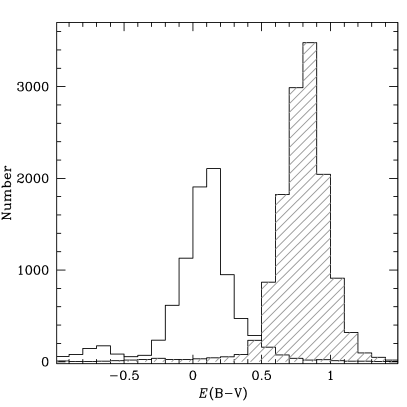
Figure 6: Results of the “blind” fit, for the stars around SN1987A: the fit described in section 4.2 is performed directly without the selection of section 4.1. Left panel: HR diagram The grey triangles highlight the stars for which the fit returns too high a value of $\mathrm{T}_{eff}$ and $E(\mathrm{B}-\mathrm{V})$. These are stars with multiple solutions for which the “blind” fit picks the wrong one (see text). The Zero Age Main Sequence for Z$=0.3\cdot\mathrm{Z}_{\sun}$ from the models by Brocato & Castellani (1993) and Cassisi et al (1994) for masses below 25 M_☉ and by Schaerer et al (1993) above 25 M_☉ is shown as a full line. Right panel: $E(\mathrm{B}-\mathrm{V})$ distribution resulting from the “blind” fit. The high reddening peak (hatched histogram) is entirely made of stars plotted in grey in the left panel, thus confirming that their location in the HR diagram is due to an erroneous reddening determination.

The HR diagram for the 21,955 stars in the field of SN1987A is displayed in Figure Accurate Stellar Population Studies from Multiband Photometric Observations^†. It is interesting to compare it to what one would have obtained from a “blind” fit of the spectrum, i.e. by skipping the selection described in section 4.1 and performing directly the 6-band fit of section 4.2. This is shown in the left panel of Figure 6.

The fit for the stars marked in grey in the left panel of Figure 6 is obviously wrong as they occupy an impossible region of the HR diagram. An inspection of the right panel of the same Figure reveals that all of these stars, and only them, were fitted with too high a value of $E(\mathrm{B}-\mathrm{V})$ and, consequently, of $\mathrm{T}_{eff}$. These are all stars that fall in regions $C$ or $D$ in Figure 3 for which the broad band spectrum can be interpreted either as a heavily reddened hot star or as a cold one with little dust in front of it. The fit just selects the solution with the lowest $\chi^{2}$, even if it is marginally lower than other possible minima. Which one of the possible solution has the lowest $\chi^{2}$ depends on such things as the $E(\mathrm{B}-\mathrm{V})$ and $\mathrm{T}_{eff}$ grids used in the fit and, in the case shown in Figure 6, the wrong one is chosen for two stars out of three. For many of these stars the available photometry is limited to F439W and redder filters. As we will see in section 7, then, the data are very little sensitive to temperature and these cold stars can be mistaken for objects as hot as 50,000 K.

On the other hand, selecting the right solution before performing the fit eliminates the problem almost completely. There still are roughly 600 stars (less than 3% of the total) under the Zero Age Main Sequence locus. However, they are mostly class IV objects, i.e. stars with very poor photometry, or stars with peculiar colors, i.e. the T Tauri stars described in detail by Panagia et al (2000) or unresolved binaries.

The stars with multiple solutions are the late-type ones. Being able to measure directly the reddening for them is important for two reasons. Firstly, as low mass stars are much more numerous than higher mass ones, the number of reddening determinations increases dramatically. In fact the late type stars for which eventually we are able to measure the reddening are typically a factor of 10 more numerous than those earlier that A0. Secondly, stars of different masses have different lifetimes and there is no a priori reason why different generations of stars should be affected by the same amount of extinction (see Zaritsky, 1999, for an example in the LMC itself). By extending our analysis to a wide range of masses we can check for population-dependent effects and deredden the different generations of stars in the most appropriate way.

In addition to measuring the intrinsic properties of the stars shown in Figure Accurate Stellar Population Studies from Multiband Photometric Observations^†, our procedure also provides individual $E(\mathrm{B}-\mathrm{V})$ measurements for more than 2,500 stars, on average one every 13 square arcseconds. The resulting histogram and spatial distribution of interstellar reddening are shown in Figure 7 (see also Panagia et al, 2000). As it can be seen, the initial suspicion is confirmed and the reddening is indeed very patchy and varies on scales of a few arcseconds.

Besides providing a very accurate reddening map, measuring individual values of $E(\mathrm{B}-\mathrm{V})$ also leads to a narrowing of the various features in the Color-Magnitude diagram, in particular the Main Sequence. This is of great help when interpreting the data, because it allows one to disentangle the broadening due to differential extinction from the one caused, for example, by the overlap of several generations of stars or by the presence of binary stars.

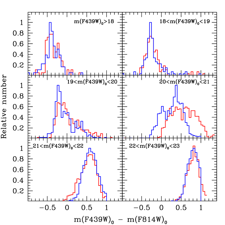
Figure 8: Width of the Main Sequence as a function of magnitude before (red line) and after (blue line) reddening correction. The magnitude interval along the Main Sequence is indicated in each panel. The faintest magnitude bin heavily suffers from incompleteness. Also, the raw histograms were shifted in color in order to have the same mode as the corrected ones. As it can be seen, the corrected histograms are systematically narrower than the uncorrected ones.

In Figure Accurate Stellar Population Studies from Multiband Photometric Observations^† we compare the stars in the F439W vs (F439W$-$F814) diagram before and after reddening correction. The density contours in panels (a) and (b) are spaced by factors of 2. Apart from the obvious fact that the corrected stars are bluer and more luminous, it is apparent that the features in the reddening corrected diagram are narrower than the corresponding ones in the observed CMD. In order to quantify this effect let us consider a color cut through the Main Sequence, like the one displayed in panel (c) of Figure Accurate Stellar Population Studies from Multiband Photometric Observations^† (see also Figure 8). Here, the blue line histogram represents the color distribution of the dereddened Main Sequence stars with $\overline{\delta}_{5}<0.1$ in the $21>$m(F439W)${}_{0}>22$ magnitude interval. The red line histogram gives the distribution of the same stars before reddening correction. To facilitate the comparison, this latter is shifted in color so as to have the same mode as the dereddened one. As apparent, the original distribution is definitely more spread out in color: its rms is 24% larger than the corrected one (0.21 mag versus 0.17). This is the case all along the Main Sequence, as shown in Figure 8, where we plot the color distribution for all the stars with $\overline{\delta}_{5}<0.1$ in different magnitude bins. The dereddened histograms (blue line) always display a smaller scatter than the observed ones (red line), confirming the effectiveness of the correction procedure.

As it can be expected, the color distribution is even narrower when only the stars with individual reddening determinations, i.e. those we have classified as class I and II, are considered. This is shown in Figure Accurate Stellar Population Studies from Multiband Photometric Observations^†. In this case the rms of the reddening-corrected Main Sequence histogram, again in the $21>$m(F439W)${}_{0}>22$ magnitude interval, is 0.14 mag, while the one of the same stars before correction is 0.18 mag, i.e. 29% larger. A simple Kolmogorov-Smirnov test shows that the widths of the two distributions are different at the 99.9995% level.

To conclude, let us remark again that Class III and IV stars were not corrected with and individually determined value of $E(\mathrm{B}-\mathrm{V})$, but, rather, with the mean value from 2,510 Class I and II neighbors. It is important to realize that, given the large number of these stars, the mean reddening used to correct Class III and IV stars is on average very accurate. Of course, it is still possible that a few class III and IV stars have, in reality, extinction values significantly different from their local mean, but the global effect is negligible.

The full discussion of the stellar content of the region around SN1987A can be found in Romaniello (1998) and Panagia et al (2000).

6 The role of gravity and metallicity

So far we have used model atmospheres only with one surface gravity ($\log(g)=4.5$, appropriate for Main Sequence stars) and metallicity (Z$=0.3\cdot\mathrm{Z}_{\sun}$, the expected mean value for the LMC). Even though these are sensible assumptions for the environment under study, we have to verify their influence on the results we derive.

Let us start by considering the surface gravity. The theoretical zero-reddening locus in the $Q_{\mathrm{UBI}}$ vs. F336W$-$F814W plane is shown in Figure 9 for three values of surface gravity, namely $\log(g)=4$ (dotted line), 4.5 (solid line) and 5 (dashed line). As it can be seen, the three curves overlap perfectly for F336W$-$F814W$\lesssim-0.5$, i.e. $\mathrm{T}_{eff}\gtrsim 11,000$ K and F336W$-$F814W$\gtrsim 1.5$, i.e. $\mathrm{T}_{eff}\lesssim 5,500$ K. Elsewhere, however, different surface gravities lead to different expected zero-reddening loci in the $Q_{\mathrm{UBI}}$ vs. F336W$-$F814W diagram. In particular, this influences the division in classes that is the foundation of the method described above.

However, as it can be seen, for example, in Figure Accurate Stellar Population Studies from Multiband Photometric Observations^†, only stars on or near the Main Sequence are used to determine the reddening. Adopting the stellar evolutionary models by Brocato & Castellani (1993) and Cassisi et al (1994), we see that for Z$=0.3\cdot\mathrm{Z}_{\sun}$ the gravity is nearly constant along the Main Sequence and that its value is $\log(g)=4.5$, the value we have used in the fit. This is a sound assumption over a large range of metallicities because extensive model calculations show that surface gravity variations as a function of chemical composition are quite small. For example, at $({\mathrm{F336W}}-{\mathrm{F814W}})_{0}=0$ the surface gravity ranges from $\log(g)\simeq 4.4$ for a solar metallicity star to $\log(g)\simeq 4.6$ for Z=Z${}_{\sun}/20$. Considering that for every metallicity the gravity is almost constant along the Main Sequence one can safely adopt the value of $\log(g)=4.5$, independent of chemical composition.

Once a star evolves off the Main Sequence its surface gravity changes appreciably. For example, $\log(g)\simeq 3$ is a typical value for the stars in the Red Giant clump, i.e. the stars at $\log(\mathrm{T}_{eff})\simeq 3.7$ and $\log(\mathrm{L}/\mathrm{L}_{\sun})\simeq 1.75$ in Figure Accurate Stellar Population Studies from Multiband Photometric Observations^†. Even though the $Q_{\mathrm{UBI}}$ vs. F336W$-$F814W relation is, indeed, sensitive to gravity, the result of our global fit is not. This is because, as we have seen, we do not fit simultaneously temperature and reddening for stars off the Main Sequence, but rather we assign to them the mean $E(\mathrm{B}-\mathrm{V})$ value of their class I and II neighbors, which are on the Main Sequence and, hence, have $\log(g)\simeq 4.5$. For stars that are off the Main Sequence, we just perform the fit to solve for the radius and effective temperature. Once the reddening is correctly determined, the result of the multi-band fit is no longer sensitive to the surface gravity adopted in computing the theoretical colors. We have checked this by dividing the stars into classes using the $Q_{\mathrm{UBI}}$ vs. ${\mathrm{F336W}}-{\mathrm{F814W}}$ relation for $\log(g)=4.5$, and then fitting the stars with colors computed for various values of the gravity. The maximum variations in temperature for the stars on the Red Giant branch are of 3%, i.e. much smaller than the error deriving from the fit itself, and with no systematic trend with gravity. Given this result, we have decided to use $\log(g)=4.5$ all throughout our analysis.

In addition to influencing the stellar structure, the chemical composition also plays a role in determining the star’s spectrum, through the atmospheric opacity. As a consequence, the colors also depend on this parameter. The $Q_{\mathrm{UBI}}$ vs. ${\mathrm{F336W}}-{\mathrm{F814W}}$ relation for different values of Z is shown in Figure 10. Again, as it can be seen, the variations are negligible for the stars for which the reddening is an individual fit parameter, i.e. Class I and II stars.

Also in this case, then, once the subdivision into classes is made and the local mean reddening for Class III and IV stars is determined from the individual values of Class I and II neighbors, the result of the multi-band fit is insensitive to the details of the stellar atmospheres. The comparison of the fits performed with colors computed for different metallicities shows that the derived parameters do not depend appreciably on metallicity.

We conclude that in applying our fitting procedure, as described in section 4, one can safely use colors computed with models by Bessel et al (1998) for Z$=0.3\cdot\mathrm{Z}_{\sun}$ and $\log(g)=4.5$ to derive accurate stellar parameters and interstellar absorptions for all stars.

7 The bands needed

For every star there are three unknown quantities: the angular radius, the effective temperature and the reddening. Therefore, for each star one needs at least data in three bands to make the problem mathematically well defined. For good results the measurements in those three bands must also be rather accurate, thus requiring that the bands be selected so as to fall around the wavelength of the maximum of the spectral distribution of any given star, and have a suitable wavelength spacing to assure a sufficient baseline for the spectral shape analysis. In practice this is achieved with bands separated from each other by about 30-40% of their central wavelengths. Moreover, when dealing with a stellar population one wants to study stars within a wide range of temperatures, and, therefore, more than three bands are absolutely needed. In this section we will investigate how many and which bands are needed to constrain the fit.

Let us start by noticing that a U-like band is mandatory to recover both $\mathrm{T}_{eff}$ and $E(\mathrm{B}-\mathrm{V})$. To illustrate this point let us define the reddening-free color $Q_{\mathrm{BVI}}$ combination of B, V and I. By analogy with equation (2):

$$Q_{\mathrm{BVI}}\equiv\left({\mathrm{B}}-{\mathrm{V}}\right)-\frac{E({\mathrm{B}}-{\mathrm{V}})}{E({\mathrm{V}}-{\mathrm{I}})}\cdot\left({\mathrm{V}}-{\mathrm{I}}\right)$$ (5)

$Q_{\mathrm{BVI}}$ is shown in Figure 11 as a function of ${\mathrm{F439W}}-{\mathrm{F814W}}$ in panel (a) and $\mathrm{T}_{eff}$ in panel (b).

Since the the B, V and I filters do not include the Balmer jump, the relation between $Q_{\mathrm{BVI}}$ and B$-I$ is monotonic, thus solving the problem of ambiguities in the solution. However, one immediately notices that the slope of the curve is much shallower than in the $Q_{\mathrm{UBI}}$ case. In fact, the total excursion of $Q_{\mathrm{BVI}}$ between 3,500 and 50,000 K is only 0.4 mag and it is almost totally insensitive to temperatures higher than 6,000 K, i.e. ${\mathrm{F439W}}-{\mathrm{F814W}}\lesssim~{}1$.

The combined effect of the weak dependence of $Q_{\mathrm{BVI}}$ on temperature and of photometric errors is to make every combination $E(\mathrm{B}-\mathrm{V})$-$\mathrm{T}_{eff}$ along the reddening vector essentially equivalent. This is shown in Figure Accurate Stellar Population Studies from Multiband Photometric Observations^† and Figure 12 where $\chi^{2}$ maps of the fit using only four bands (F439W, F555W, F675W, and F814W, left panel) are compared to those using all six of them (right panel). As it can be seen, when only 4 bands are used the $\chi^{2}$ has no distinct minima, and, hence, it is not possible to determine both the reddening and the temperature neither for hot stars for which the solution is unambiguous (Figure Accurate Stellar Population Studies from Multiband Photometric Observations^†) nor for the cold ones with multiple minima (Figure 12).

Also, let us notice here that, while observations at wavelengths shorter than the Balmer jump are mandatory to recover both $\mathrm{T}_{eff}$ and $E(\mathrm{B}-\mathrm{V})$, it is preferable not to go too far in the ultraviolet, unless one can afford to make observations in more than one UV band. Qualitatively, the reason for this is that shorter wavelengths are more affected by interstellar reddening and small differences in $E(\mathrm{B}-\mathrm{V})$ along different lines of sight may result in large differences in the observed flux, thus making the ultraviolet flux of a moderately reddened hot star almost indistinguishable from the one of an unreddened, colder one. Quantitatively, the situation is illustrated in Figure 13, where we plot the $1\sigma$ contour levels for artificial stars of different effective temperature as observed through 4 optical filters (F439W, F555W, F675W and F814W) and one UV one: F170W (dot-dashed line), F255W (dashed line) or F336W (full line). The contours, computed assuming the same photometric error in all 3 UV filters, overlap almost perfectly. This means that one does not gain in accuracy by observing at shorter wavelengths, even for hot stars. Since the sensitivity of normal CCDs and the emission of cold stars both drop dramatically the further one moves to the ultraviolet, a filter in the region of the U band is the ideal choice for the filter bluer of the Balmer jump.

As we have pointed out at the beginning of this section, there are 3 unknowns in the fit so that 6 bands are actually redundant and 4 could be enough to cover the wide range of temperatures spanned by stars in regions with mixed stellar populations. In fact, the method works rather well also with only 4 bands, provided that they encompass the Balmer jump. This is shown in Figure Accurate Stellar Population Studies from Multiband Photometric Observations^†, where the HR diagram for the control field located $8^{\prime}$ south-east of SN1987A, derived following our procedure, is shown. In this case, as reported in Table 2, the four available photometric bands were F300W, F450W, F675W and F814W. The star symbol shows the location of the brightest star in the WFPC2 field of view. It is so heavily saturated in the WFPC2 chip that its image was spilling over several neighboring stars thus making impossible to make direct measurements, and, therefore, its photometry is taken from Fitzpatrick (1998).

As it can be seen, the observed Main Sequence, although still in very good agreement with the theoretical one, is less sharply defined than the one in the field of SN1987A (see Figure Accurate Stellar Population Studies from Multiband Photometric Observations^†) and more stars fall under the theoretical ZAMS. Using a reduced set of filters has affected the result in two ways. Firstly, there is only one band blueward of the Balmer jump (F300W) instead of two (F255W and F336W): the fit is less sensitive to temperature for hot stars and, hence, for them, the results are less accurate. Secondly, since the observations were taken as “parallels” to FOS primaries, we did not have enough time to make observations both in the F555W, or a similar band like F606W, and in the F675W filter. We opted for this latter one to identify stars with $\mathrm{H}\alpha$ emission more accurately. As a result, though, the photometric points are not spaced in wavelength quite evenly. As a consequence, the fit for the cooler stars, the ones that are not well exposed in F300W and F450W bands, has to rely on a short wavelength baseline and, thus, is less precise than it would have been if observations at roughly 5000 Å had been available. This also results in a larger fraction of stars below the Main Sequence (roughly 600 out of a total of nearly 13,100, i.e. 4.6%) when compared to the main field (roughly 600 out of almost 22,000, i.e. less than 3%). In general, however, the resulting stellar parameters are still of very good quality, with more than 30% of the stars with an error in $\mathrm{T}_{eff}$ smaller than 10%.

8 The effect of random and systematic photometric errors

In order to assess the intrinsic precision of the procedure described in this paper we have tested it on simulations. Artificial stars were created with ${E(\mathrm{B}-\mathrm{V})}=0.2$ in the 6 filters listed in Table 1, evenly distributed in the logarithm of effective temperature between 3,500 and 50,000 K, the range covered by Bessel et al (1998) models. They were, then, fitted according to the prescriptions of section 4.

8.1 Random errors

The effects of random errors were mimicked by creating three groups of 10,000 stars and adding to the model magnitudes errors drawn from Gaussians of different rms (0.02, 0.05 and 0.1 mag). These stars were then fitted using only 4, 5 or the complete set of 6 bands.

The situation for a five-band fit (F336W, F439W, F555W, F675W and F814W) and varying the photometric precision is shown in Figure Accurate Stellar Population Studies from Multiband Photometric Observations^†. There we plot the ratio of the output to input temperature as a function of the input temperature for different values of the error rms: 0.1 mag in panel (a), 0.05 mag in panel (b) and 0.02 mag in panel (c). In each panel the photometric errors were drawn from the same Gaussian, independent of the star’s temperature. As it can be seen, there is no systematic trend and the points are mostly scattered around $\mathrm{T_{out}}=\mathrm{T_{in}}$. The values of the mean and the dispersion are reported in Table 5.

The biggest deviation from the random scatter is represented by the two features at $\log(\mathrm{T_{in}})\simeq 3.95$, which are most prominent in panel (c). These are stars close to the turning point at ${\mathrm{F336W}}-{\mathrm{F814W}}\simeq 0$ in Figure 3 and were assigned the wrong value of $E(\mathrm{B}-\mathrm{V})$ during the selection process which constitutes the first step of the procedure. Note that this effect depends on the input photometric error because the class assignment is based on it. In the worst case, when the error is 0.02 mag, however, this systematics affects less than 10% of the stars at that temperature, split almost evenly between stars with too high and too low output temperature. This effect is negligible for studies of stellar populations. However if one is dealing with special categories of objects, for example variable or otherwise peculiar stars, which represent a small fraction of the total population in the $3.92\lesssim\log(\mathrm{T}_{eff})\lesssim 4$ range one should be aware that random errors may create false outliers with temperatures deviating as much as 20% for up 10% of the stars in this temperature range. For this type of studies it is safer not to determine extinction for individual stars but, rather, to adopt the value of the neighbors not affected by this problem.

It is interesting to notice in all of the panels in Figure Accurate Stellar Population Studies from Multiband Photometric Observations^† that the dispersion increases for hotter stars. This is because broad band colors become progressively more insensitive to temperature as it increases. In fact, the scatter at high temperatures becomes smaller when the F255W filter is added to the fit, as shown in Figure Accurate Stellar Population Studies from Multiband Photometric Observations^†. Of course, in reality hotter Main Sequence stars are also brighter than colder ones and, thus, have smaller photometric error which compensate for the lower sensitivity of colors to high effective temperatures. Again, see Table 5 for the values of the mean and dispersion.

8.2 Systematic errors

In addition to random errors that vary from star to star and from band to band the measured fluxes are also affected by systematic errors in the calibrations of each band, i.e. errors in the photometric zeropoints. These, of course, are different from band to band, but the same for all the stars in each band. Again, we have explored three cases (0.02, 0.05 and 0.1 mag) and the results are shown in Figure 14 that displays the distributions of the temperature deviations $\log(\mathrm{T_{out}}/\mathrm{T_{in}})$ for four representative temperatures, i.e. 5,000, 10,000, 20,000 and 40,000 K.

From an inspection of Figure 14 one notices again that, given the same error, the temperature measured for hot stars is intrinsically more uncertain than for cold ones, with the dispersion growing from less than 1% for stars at 5000 K, to as much as 12% at 40,000 K. The sharp peak at $\log(\mathrm{T_{out}/T_{in}})\simeq 0.1$ found for $\mathrm{T_{in}}=40,000$ K (Figure 14, panel (d)) is populated by stars for which the fit, starting from $\mathrm{T_{in}}=40,000$ K, would indicate a temperature higher than 50,000 K, the highest in the Bessel et al (1998) grid. Even though the peak is just an artifact, it is clear that calibration errors much smaller than 0.1 mag are necessary for the data to be useful at all temperatures.

9 Summary and conclusions

In this paper we have presented and discussed a new technique that uses multiband photometry to measure reddening, effective temperature and, given the distance, bolometric luminosity for resolved stars. The method is based on broad band optical and near ultraviolet photometry and, in the test case presented here for the field around SN1987A in the Large Magellanic Cloud, yields to a reddening determination every 13 square arcseconds: a fine grid indeed! Being able to measure the reddening to thousands of individual stars is of great importance in all the astrophysical environments in which the interstellar medium is clumpy and, therefore, produces differential reddening, as is the case, for example, of virtually every star forming region.

There are 3 unknown quantities in the fit: the radius, the effective temperature and the reddening. Formally, then, at least three photometric points are required for each star to make the problem well defined, and more are needed when dealing with stellar population encompassing a wide range of temperatures. Obviously, the more bands are available, the better the result of the fit. As we have discussed thoroughly, at least one of the bands has to fall at wavelengths shorter than the Balmer jump because the optical fluxes alone are not enough to reliably recover both $\mathrm{T}_{eff}$ and $E(\mathrm{B}-\mathrm{V})$. On the other hand, though, in the case in which observing time constraints limit to one the the number of bands that can be used for UV observations, it is not necessary nor advisable to resort to bands at extremely short wavelengths, and observing just blueward of the Balmer jump, a U-like band, is the best choice. Of course, observing in more than one ultraviolet band can only help in reducing the errors on the derived quantities. Although we have used the WFPC2 counterparts to the classical Johnson-Cousin passbands to illustrate our method, it proved to work almost equally well when broader filters were used. Broader filters means more photons detected per unit time and, ultimately, a more efficient use of the telescope time at one’s disposal.

Once the stars are accurately placed in the Hertzprung-Russel diagram, the physical properties of the stellar population, such as star formation history, mass function etc, can be studied in detail. In this respect, let us stress again the importance of determining the reddening from the same stars which are the ultimate target of the investigation, without having to resort to uncontrollable assumptions on the magnitude and distribution of the interstellar extinction.

To conclude, we refer the reader to Panagia et al (2000) for a discussion of the properties of the young stellar population in the field around SN1987A and to Romaniello et al (2000) for an application of the dereddend Color-Magnitude diagram to measuring the distance to the Large Magellanic Cloud. More work on the derivation of the Initial Mass Function and the Star Formation Rate in the SN 1987A field is in progress, and the results will be presented in a forthcoming paper Romaniello et al (2002).

Appendix A: The fitting procedure

As repeatedly stated, the general idea of our method is to recover simultaneously the extinction along the line of sight and the effective temperature of a star by fitting the observed magnitudes to the ones computed using stellar atmosphere models reddened by various amounts of $E(\mathrm{B}-\mathrm{V})$. In this Appendix we describe the details of the fitting procedure.

Among the three parameters we want to determine, only two change the shape of the spectrum, i.e. $E(\mathrm{B}-\mathrm{V})$ and effective temperature ($\mathrm{T}_{eff}$). The third one, i.e. the radius $R$, causes just a rigid shift of the flux on a logarithmic scale. So, we first determine the shape of the spectrum by solving simultaneously for $E(\mathrm{B}-\mathrm{V})$ and $\mathrm{T}_{eff}$, then we compute the radius of the star. For every star, the following steps are performed:

1. The input spectrum is normalized to the band with the highest photometric accuracy, usually the F555W, to eliminate the overall normalization, which depends an the star’s radius. Obviously, the theoretical spectra are normalized in the same way. Let $m_{obs,i}$ be the normalized observed magnitude in filter $i$ and $m^{0}_{ms,ij}$ the normalized model magnitude for temperature $j-th$ in the same filter;

2. The theoretical magnitudes are reddened, for various values of $E(\mathrm{B}-\mathrm{V})$. If $\mathcal{R}_{i}$ is the extinction coefficient in the band $i$ due to the LMC dust and $\mathcal{R}_{i,\mathrm{MW}}$ is the one due to our Galaxy:

   $$m_{ms,ij}\left[{E(\mathrm{B}-\mathrm{V})}\right] =m_{ms,ij}^{0}+\left[\mathcal{R}_{i}\cdot{E(\mathrm{B}-\mathrm{V})}\right]+$$ (6)

   $$\left[\mathcal{R}_{i,\mathrm{MW}}\cdot{E(\mathrm{B}-\mathrm{V})}_{\mathrm{MW}}\right]$$

   with ${E(\mathrm{B}-\mathrm{V})}_{\mathrm{MW}}=0.05$, as already discussed. The extinction coefficients for selected WFPC2 filters are listed in Table 8;

3. For any given temperature and reddening, we have computed the $\chi^{2}$ as:

   $$\chi_{j}^{2}\left[{E(\mathrm{B}-\mathrm{V})}\right]=\sum_{i=1}^{N-1}\left[\frac{m_{ms,ij}\left[{E(\mathrm{B}-\mathrm{V})}\right]-m_{obs,i}}{\delta m_{obs,i}}\right]^{2}$$ (7)

   where $N$ is the number of photometric points and $\delta m_{obs,i}$ is the error on the observed magnitude $m_{obs,i}$. The quantity $\delta m_{obs,i}$, of course, is the sum in quadrature of the photometric error on the magnitude in band $i$ plus the one on the magnitude in the band to which the spectrum was normalized. The index $i$ in the sum runs on all bands, but the one that was used to normalize the spectrum. If a star is not detected in a certain band, typically in the UV, a $3\sigma$ upper limit for the flux is used. The models that predict a flux in that band higher than this limit are rejected.

   Of course, the best-fit model corresponds to the combination temperature, and $E(\mathrm{B}-\mathrm{V})$ that minimizes $\chi_{j}^{2}\left[{E(\mathrm{B}-\mathrm{V})}\right]$;

4. Once the minimum $\chi_{j}^{2}$ is found, the errors in temperature ($\delta\mathrm{T}_{eff}$) and reddening ($\delta{E(\mathrm{B}-\mathrm{V})}$) are computed from the $\chi^{2}$ map;

5. Now that the shape of the spectrum is determined, we compute the radius of the star as the error-weighted mean of the logarithmic shifts required to match the model to the observed flux in every band. Since the theoretical fluxes are flux densities at the surface of the star, the angular radius $\rho$ derived from band $i$ is:

   $$\log\left(\rho_{i}\right)=-0.2\cdot\left(m_{obs,i}^{0}-m_{ms,i}^{fit}\right)$$ (8)

   where $m_{ms,i}^{fit}$ is the magnitude in filter $i$ of the best-fitting theoretical spectrum and $m_{obs,i}^{0}$ is the observed magnitude, dereddened with the the best-fitting value of $E(\mathrm{B}-\mathrm{V})$. The best estimate of the angular radius $\rho$, then, is:

   $$\rho=\frac{\sum_{i=1}^{n}\rho_{i}/\delta^{2}m_{obs,i}}{\sum_{i=1}^{n}1/\delta^{2}m_{obs,i}}$$ (9)

   where $n$ is the number of bands with actual flux measurements. The associated error $\delta\rho$, then, is:

   $$\left(\delta\rho\right)^{2}=\frac{\sum_{i=1}^{n}\left(\rho_{i}-\rho\right)^{2}/\delta^{2}m_{obs,i}}{(n-1)\cdot\sum_{i=1}^{n}1/\delta^{2}m_{obs,i}}$$ (10)

   To convert the angular radius of a star to the linear one ($R$), it is necessary to know its distance $D$:

   $$R=\rho\cdot\frac{D}{\mathrm{R}_{\sun}}$$ (11)

   in this case, $R$ is expressed in units of the solar radius R_☉.

   Given the uncertainty on the distance, the error on the linear radius ($\delta R$) is:

   $$\frac{\delta R}{R}=\sqrt{\left(\frac{\delta\rho}{\rho}\right)^{2}+\left(\frac{\delta D}{D}\right)^{2}}$$ (12)

   This error does not take into account any intrinsic dispersion in the distance of individual stars, which may introduce additional scattering in the HR diagram.

   For example, in the case of the LMC, we have adopted the value originally measured purely geometrically by Panagia et al (1991) and later improved by Panagia (1999). Using the rings around SN1987A, they found $D=51.4\pm 1.2$ kpc;

6. Finally, the intrinsic luminosity (L) can be computed according to the black body law:

   $$\frac{\mathrm{L}}{\mathrm{L}_{\sun}}=\left(\frac{R}{\mathrm{R}_{\sun}}\right)^{2}\cdot\left(\frac{\mathrm{T}_{eff}}{\mathrm{T}_{eff,\odot}}\right)^{4}$$ (13)

   where $\mathrm{T}_{eff,\odot}$ is the temperature of the Sun.

   Since the errors in temperature and radius are correlated, the error on the luminosity cannot be computed in a straightforward way from the previous equation. It is more convenient to write the luminosity in another, completely equivalent form. Let us first define the quantities:

   $$l_{obs,i}\equiv 10^{-0.4\cdot\left(m_{obs,i}^{0}-ZP_{i}\right)}$$ (14)

   i.e. the observed flux in filter $i$, and:

   $$b\equiv\frac{\sigma\,\mathrm{T}_{eff}^{4}}{\sum_{i=1}^{n}l_{ms,i}^{fit}}$$ (15)

   where $l_{ms,i}^{fit}$ is the flux in filter $i$ of the best-fitting model. The quantity $b$ is the equivalent of the bolometric correction, relating the total flux in $n$ bands to the bolometric luminosity per unit surface $\sigma\mathrm{T}_{eff}^{4}$. We can now write the luminosity as:

   $$L=4\pi D^{2}\>l_{obs}\>b$$ (16)

   where $l_{obs}=\sum_{i}l_{obs,i}$. All the quantities in this last equation are independent from each other and, hence, it is straightforward to compute the error on the luminosity:

   $$\frac{\delta L}{L}=\sqrt{\left(2\,\frac{\delta D}{D}\right)^{2}+\left(\frac{\delta l_{obs}}{l_{obs}}\right)^{2}+\left(\frac{\delta b}{b}\right)^{2}}$$ (17)

   where

   $$\frac{\delta l_{obs}}{l_{obs}}=\frac{1}{l_{obs}}\sqrt{\sum_{i=1}^{n}\left[\left(10^{0.4\delta m_{obs,i}}-1\right)\cdot l_{i,obs}\right]^{2}}$$ (18)

   and:

   $$\frac{\delta b}{b}=\frac{db}{d\mathrm{T}_{eff}}\>\delta\mathrm{T}_{eff}$$ (19)

   In this last equation, it is clear that the first term on the right-hand side, $db/d\mathrm{T}_{eff}$, is completely determined by the models, whereas the second one, $\delta\mathrm{T}_{eff}$, is the error on the temperature from the fit computed in step 4.

   In the case of the LMC, $\delta D/D=0.02$ (Panagia, 1999).

   Let us stress once again that the stars may not be all at the same distance and that this may introduce additional scattering in luminosity. From photometry alone, distances can be measured only in a statistical sense for an entire population and not for individual stars. However, since the intrinsic depth the LMC is estimated to be smaller than 600 pc (Crotts et al, 1995), this uncertainty is negligible.

AppendixB: Broad band colors and extinction coefficients in selected WFPC2 filters

The WFPC2 is equipped with a large set of broad, medium and narrow band filters for imaging (see Biretta et al, 2000, for a complete list and full details). Some of them closely match filters in the standard Johnson-Cousin (e.g. the F555W and the V, the F439W and the B, etc) or Strömgren (e.g. the F410M and the v, the F467M and the b, etc) systems, while some other have no direct counterpart in any standard ground-based set, e.g., the F450W and F606W, just to name two, or, obviously, all ultraviolet passbands.

Color transformations have been devised to convert the WFPC2 magnitudes into the corresponding ones in the Johnson-Cousin system, but, they are limited to only a handful of passbands. Moreover, quoting directly from Biretta et al (2000), they “should be used with caution for quantitative work”, because they are just first order approximations and unavoidably degrade the quality of the original photometry. A much better option, when comparing WFPC2 photometry to theoretical expectations, is to compute these latter ones directly in the passbands used in the observations. As explained in section 4, this is what we have done in this paper, thus minimizing the uncertainties in the comparison between the observed WFPC2 magnitudes and the synthetic ones computed using the Bessel et al (1998) models.

In Tables 6 and 7 we list the magnitudes in widely used WFPC2 passbands for solar metallicity and for [Fe/H]$=-0.5$, the appropriate value for the LMC, respectively. They were computed using the IRAF-synphot synthetic photometry package and, for the sake of generality, the magnitudes in the ultraviolet filters are referred to the decontaminated camera. The throughput degradation due to the accumulation of material between decontamination can be easily computed with the formulæ given in Bagget et al (1996). The magnitudes are for a 1 R_☉ star as seen from a distance of 10 pc and scaling them for any radius and distance using equation (20) is straightforward.

The other important quantities that one needs in order to interpret the data are the extinction coefficients. Again, it is very important to compute them in the very same passbands used for the observations. The values of the normalized extinction $\mathcal{R}_{\lambda}=A_{\lambda}/E(B-V)$ for the filters of Tables 6 and 7 computed for the galactic reddening law as compiled by Savage & Mathis (1979) and the models atmospheres by Bessel et al (1998) are listed in Table 8 for various values of the effective temperature and the color excess $E(\mathrm{B}-\mathrm{V})$.

Using the entries of Tables 6, 7 and 8, then, it is very easy to model a star of metallicity Z, surface gravity $g$, effective temperature $\mathrm{T}_{eff}$, radius $R$ (in solar units) as seen at a distance $D$ (in parsecs) through a layer of dust characterized by a reddening $E(\mathrm{B}-\mathrm{V})$:

$$m(\mathrm{Z},g,\mathrm{T}_{eff},R,D,{E(\mathrm{B}-\mathrm{V})})=m_{0}(\mathrm{Z},g,\mathrm{T}_{eff})+$$

$$-5\cdot\left(\frac{R}{1~{}\mathrm{R}_{\sun}}\right)+5\cdot\log\left(\frac{D}{10~{}pc}\right)$$

$$+\mathcal{R}(\mathrm{T}_{eff},{E(\mathrm{B}-\mathrm{V})})\cdot{E(\mathrm{B}-\mathrm{V})}$$ (20)

where $m_{0}(\mathrm{Z},g,\mathrm{T}_{eff},Z)$ is the appropriate value, either read or interpolated from Table 6 or 7, and $\mathcal{R}(\mathrm{T}_{eff},{E(\mathrm{B}-\mathrm{V})})$ can be taken from Table 8.

Ultraviolet WFPC2 filters are notoriously affected by red leak, and a quite substantial one when red stars are observed (see table 3.13 of Biretta et al, 2000). This is the reason why, for example, as shown in Table 8, the extinction coefficient $\mathcal{R}$ in the F170W filter is about 4 times smaller for a $\mathrm{T}_{eff}=3,500$ K star than for a 40,000 K one! One can easily assess the influence of the red leak by recomputing the same coefficients after cutting it out from the response curve of the filter, in this case the F170W. What one finds, then, is that, while the extinction coefficient for $\mathrm{T}_{eff}=40,000$ K is virtually unchanged, the one for $\mathrm{T}_{eff}=3,500$ K increases by a factor of 3, thus reducing the difference between them to about 30%. The residual difference in $\mathcal{R}$ between different temperatures, the lower one yielding to lower extinction coefficients, is caused by the fact that filters have a finite, non negligible bandwidth and, thus, the effective extinction in a band depends on the shape of the spectrum which is a function of temperature. The same explanation applies for the fact (also illustrated in Table 8) that extinction coefficients become smaller as the optical depth of the dust increases because dust extinction makes a spectral energy distribution become redder.

Tables with similar quantities computed for all of WFPC2 filters and for all model atmospheres in the Bessel et al (1998) grid are available and may be provided on request.

See fig01.jpg

The field centered on SN1987A (about 130^′′ radius) as observed in the combination of the B, V, and I broad bands plus the [OIII] and H$\alpha$ narrow band images.

See fig02.jpg

Color-Magnitude Diagrams for four combination of filters. The grey dots are stars with average errors, as defined in equation (1), $\overline{\delta}_{5}>0.1$, whereas the black dots are the 6,695 stars with $\overline{\delta}_{5}<0.1$. The reddening vector corresponding to ${E(\mathrm{B}-\mathrm{V})}=0.2$ is show in each panel

See fig03.jpg

Photometric error as a function of magnitude for the 6 broad band filters around SN1987A. The 0.1 mag error level is indicated.

Figure 1: Four examples of the spectral resolution of the “Wide Band spectroscopy”. The magnitudes and errors of these four stars are given in Table 3. The position of the Balmer jump at 3646 Å is indicated with a dashed line.

Figure 2: Comparison of spectra for different combinations of $\mathrm{T}_{eff}$ and $E(\mathrm{B}-\mathrm{V})$: $\mathrm{T}_{eff}=5,000$ and ${E(\mathrm{B}-\mathrm{V})}=0$ (short-dash line), $\mathrm{T}_{eff}=7,600$ and ${E(\mathrm{B}-\mathrm{V})}=0.55$ (long-dash line), $\mathrm{T}_{eff}=12,000$ and ${E(\mathrm{B}-\mathrm{V})}=0.86$ (full line). The spectra are normalized to the F814W flux and errorbars corresponding to 0.1 mag are shown. As it can be seen, at this resolution the spectra are almost indistinguishable for wavelengths longer than 3,300 Å and ultraviolet imaging is needed to tell them apart.

Figure 3: Reddening-free color $Q_{\mathrm{UBI}}$ as a function of $({\mathrm{F336W}}-{\mathrm{F814W}})$ from the theoretical models by Bessel et al (1998) for Z$=0.3\cdot$Z_☉ and $\log(g)=4.5$. The horizontal arrow indicates the reddening vector for ${E(\mathrm{B}-\mathrm{V})}=0.2$ mag and a few important temperatures along the sequence are also marked. Stars in the four regions $A\rightarrow D$ have a different number of solutions (see text). The dashed line highlights the location in this diagram of the T Tauri stars: their colors are not well represented by normal photospheres.

Figure 4: Location of class I (filled circles), II (filled triangles) and III (small dots) stars in the $Q_{\mathrm{UBI}}$ vs. ${\mathrm{F336W}}-{\mathrm{F814W}}$ plane.

Figure 5: Same as Figure 1, but with the best fitting model shown as a full line. The parameters derived from the fit are listed in Table 4.

See fig09.jpg

HR diagram for the stars in the field around SN1987A. The black dots are the 9,474 stars with $\delta\log(\mathrm{T}_{eff})<0.05$. The Zero Age Main Sequence for Z$=0.3\cdot\mathrm{Z}_{\sun}$ from the models by Brocato & Castellani (1993) and Cassisi et al (1994) for masses below 25 M_☉ and by Schaerer et al (1993) above 25 M_☉ is shown as a full line.

See fig10a.jpg

Figure 7: Panel (a): reddening histogram from the stars in the field of Supernova 1987A. Only stars for which $E(\mathrm{B}-\mathrm{V})$ was measured individually (the 2,510 class I and II stars, see the text) are used here. Panel (b): spatial distribution of stars with high (${E(\mathrm{B}-\mathrm{V})}>0.3$, filled circles) and low (${E(\mathrm{B}-\mathrm{V})}<0.1$, open circles) reddening.

See fig12.jpg

Before and after the reddening correction. The observed $\mathrm{F439W}$ vs. ${\mathrm{F439W}}-{\mathrm{F814W}}$ diagram for all the stars in our WFPC2 frames with $\overline{\delta}_{5}<0.1$ is shown in panel (a), while the dereddened one in panel (b). Black dots represent the stars for which $E(\mathrm{B}-\mathrm{V})$ was determined individually (class I and II, see text), grey dots stars dereddened with the mean value of $E(\mathrm{B}-\mathrm{V})$ from the closest class I and II neighbors. The density contours, spaced by factors of 2, are are superposed in red. The visual impression that the Main Sequence in panel (b) is narrower than the one in panel (a) is confirmed by the histograms shown in panel (c). Here, the blue line represents the color distribution of the dereddened stars in the $21<\mathrm{m(F439W)_{0}}<22$ magnitude interval and the red one the distribution of the observed colors for the same stars. For the sake of clarity, the latter was shifted by 0.5 mag in color to have the same mode of the dereddened one. There are 218 and 192 stars, respectively, at the peak of the dereddened and observed distribution, while both histograms contain a total of 1923 stars.

See fig14.jpg

Same as Figure Accurate Stellar Population Studies from Multiband Photometric Observations^†, but the contours in panels (a) and (b) and the histograms in panel (c) refer only to the stars with individual reddening correction (class I and II, see text). The peak values of the histograms in panel (c) are 174 and 141 for the corrected (blue line) and observed one (red line), respectively.

Figure 9: Zero-reddening $Q_{\mathrm{UBI}}$ vs. ${\mathrm{F336W}}-{\mathrm{F814W}}$ relation for three values of surface gravity: $\log(g)=5$ (dashed line), $\log(g)=4.5$ (solid line) and $\log(g)=4$ (dotted line). The model atmospheres are those of Bessel et al (1998) for Z$=0.3\cdot\mathrm{Z}_{\sun}$. The points for $\mathrm{T}_{eff}$=50,000, 15,000, 9,250, 6,000 and 3,500 K are marked on each curve.

Figure 10: Zero-reddening $Q_{\mathrm{UBI}}$ vs. ${\mathrm{F336W}}-{\mathrm{F814W}}$ relation for three values of metallicity: Z=Z_☉ (dashed line), Z$=0.3\cdot\mathrm{Z}_{\sun}$ (solid line) and Z=Z${}_{\sun}/10$ (dotted line). The model atmospheres are those of Bessel et al (1998) for $\log(g)=4.5$. The points for $\mathrm{T}_{eff}$=50,000, 15,000, 9,250, 6,000 and 3,500 K are marked on each curve.

Figure 11: The $Q_{\mathrm{BVI}}$ reddening-free color as a function of ${\mathrm{F439W}}-{\mathrm{F814W}}$ (panel (a)) and $\mathrm{T}_{eff}$ (panel (b)) for the Bessel et al (1998) model atmospheres for Z$=0.3\cdot$Z_☉ and $log(g)=4.5$. The case of black body spectra is shown in both panels as a dashed line.

See fig18b.jpg

Contour plots in the $\mathrm{T}_{eff}$-$E(\mathrm{B}-\mathrm{V})$ space for four stars with unambiguous solution. Left panel: only four bands (F439W, F555W, F675W and F814W) are used in the fit. Right panel: all six bands are used. In both panels the contours are for $\delta\chi^{2}=2$ from the minimum.

See fig19b.jpg

Figure 12: Same as Figure Accurate Stellar Population Studies from Multiband Photometric Observations^†, but for stars with multiple solutions.

Figure 13: $\chi^{2}$ contour map for artificial stars with ${E(\mathrm{B}-\mathrm{V})}=0.2$ and $\mathrm{T}_{eff}=20,000~{}\mathrm{K~{}(panel~{}(a))}$, 25,000 K (b), 30,000 K (c) and 40,000 K (d). The contours correspond to the $1\sigma$ confidence level for a 5-band fit. In all cases the same 4 optical filters are used (F439W (B), F555W (V), F675W (R) and F814W (I)) in combination with different UV passbands: F170W (dot-dashed line), F255W (dashed line) or F336W (full line). The photometric error is assumed to be the same in all 3 UV filters. The thin straight lines mark the input parameters of the model stars.

See fig21.jpg

HR diagram for the 13,098 stars detected in the control field for SN1987A. Black dots are the 4,912 stars with $\delta\log(\mathrm{T}_{eff})<0.05$. The open squares indicate stars for which the F300W magnitude is ill determined because of saturation and, hence, the fit was performed excluding this filter. The location of Sk -69 211 according to the photometry by Fitzpatrick (1998) is shown with a star symbol. The Zero Age Main Sequence for Z$=0.3\cdot\mathrm{Z}_{\sun}$ from the models by Brocato & Castellani (1993) and Cassisi et al (1994) for masses below 25 M_☉ and by Schaerer et al (1993) above 25 M_☉ is shown as a full line.

See fig22.jpg

Ratio of output to input temperature as a function of the latter for 10,000 model stars distributed evenly in $\log(\mathrm{T_{in}})$. The fit was performed as described in section 4 using 5 bands: F336W, F439W, F555W, F675W and F814W. The input stars in panel (a) simulate a random photometric error of 0.1 mag in all of the bands, those in panel (b) an error of 0.05 mag and those in panel (c) an error of 0.02 mg. Black dots are class I and II stars for which the reddening was determined individually, while grey ones are class III stars dereddened with the average value of their class I and II neighbors.

See fig23.jpg

Same as Figure Accurate Stellar Population Studies from Multiband Photometric Observations^†, but the fit was performed with different combinations of bands: 4 in panel (a) (F336W, F439W, F555W and F814W), 5 in panel (b) (those of panel (a) plus F675W) and 6 in panel (c) (those of panel (b) plus F255W). The stars simulate a random photometric error of 0.05 mag.

Figure 14: Distribution of the ratio of output to input temperature in the case of systematic errors for four representative temperatures: 5,000 K in panel (a), 10,000 K in panel (b), 20,000 K in panel (c) and 40,000 K in panel (d). In each panel the dotted line is for the case of a systematic error of 0.02 mag, the full one for 0.05 mag and the dashed one for 0.1 mag.

Table 1: Log of the observations centered on Supernova 1987A.

Filter Name	Exposure Time (seconds)			Comments
	September 1994	February 1996	July 1997
F255W	2x900	1100+1400	2x1300	UV Filter
F336W	2x600	2x600	2x800	U Filter
F439W	2x400	350+600	2x400	B Filter
F555W	2x300	2x300	2x300	V Filter
F675W	2x300	2x300	2x300	R Filter
F814W	2x300	2x300	2x400	I Filter

Table 2: Log of the observations of the control field for SN1987A. They were taken on January, 1^st 1997 and the proposal number is 6437.

Filter Name	Exposure Time (s)	Comments
F300W	$600+1200$	Wide U filter
F450W	$50+200$	Wide B filter
F675W	$50+200$	R filter
F814W	$140+400$	I filter

Table 3: Observed magnitudes and statistical errors for the stars of Figure 1.

Panel	F255W	F336W	F439W	F555W	F675W	F814W
(a)	$15.74\pm 0.01$	$16.13\pm 0.01$	$17.37\pm 0.01$	$17.23\pm 0.01$	$17.44\pm 0.01$	$17.48\pm 0.01$
(b)	$19.34\pm 0.04$	$19.24\pm 0.01$	$19.83\pm 0.01$	$19.69\pm 0.01$	$19.45\pm 0.01$	$19.28\pm 0.01$
(c)	$21.50\pm 0.20$	$20.99\pm 0.03$	$20.91\pm 0.02$	$20.71\pm 0.01$	$20.45\pm 0.01$	$20.35\pm 0.01$
(d)	$22.10\pm 0.30$	$21.32\pm 0.04$	$21.23\pm 0.02$	$20.85\pm 0.01$	$20.46\pm 0.01$	$20.26\pm 0.01$

Table 4: Best-fit parameters for the spectra of Figure 5. The star in panel (a) is saturated and this causes the large quoted errors on the quantities derived for it. The corresponding magnitudes are listed in Table 3.

Panel	$\mathrm{T}_{eff}$(K)	$E(\mathrm{B}-\mathrm{V})$	log(L/L☉)	R/R☉
(a)	$25,350\pm 5,700$	$0.202\pm 0.080$	$3.662\pm 0.264$	$3.444\pm 0.090$
(b)	$18,160\pm 2,100$	$0.431\pm 0.051$	$2.695\pm 0.166$	$2.265\pm 0.050$
(c)	$8,000\pm 350$	$0.117\pm 0.050$	$1.176\pm 0.079$	$2.070\pm 0.042$
(d)	$7,480\pm 300$	$0.209\pm 0.047$	$1.255\pm 0.067$	$2.548\pm 0.052$

Table 5: Mean ratio and rms scatter of the output to input values of selected quantities for 10,000 artificial stars (see text).

Input	Fitted	$\mathrm{T}_{eff}$		$E(\mathrm{B}-\mathrm{V})$		L
error	bands	$\mathrm{T_{in}}<9,000$	$\mathrm{T_{in}}>9,000$	$\mathrm{T_{in}}<9,000$	$\mathrm{T_{in}}>9,000$	$\mathrm{T_{in}}<9,000$	$\mathrm{T_{in}}>9,000$
(rms)
0.1	5	$0.99\pm 0.05$	$0.97\pm 0.18$	$0.01\pm 0.02$	$-0.02\pm 0.06$	$0.98\pm 0.17$	$1.01\pm 0.58$
0.05	5	$0.99\pm 0.03$	$0.98\pm 0.12$	$0.01\pm 0.02$	$-0.01\pm 0.04$	$0.97\pm 0.10$	$0.99\pm 0.37$
0.02	5	$0.99\pm 0.04$	$0.99\pm 0.06$	$0.01\pm 0.03$	$-0.00\pm 0.02$	$0.97\pm 0.11$	$0.97\pm 0.18$
0.05	4	$0.99\pm 0.04$	$0.98\pm 0.12$	$0.01\pm 0.02$	$-0.01\pm 0.04$	$0.98\pm 0.11$	$0.99\pm 0.38$
0.05	6	$1.00\pm 0.03$	$0.98\pm 0.11$	$0.01\pm 0.02$	$-0.01\pm 0.04$	$0.99\pm 0.10$	$0.97\pm 0.35$

Table 6: Magnitudes in selected WFPC2 broad band filters from the Bessel et al (1998) models for Z=Z${}_{\sun}=0.02$ referred to a 1 R_☉ star at a distance of 10 pc (see equation (20)).

$\mathrm{T}_{eff}$	F170W	F255W	F300W	F336W	F439W	F450W	F555W	F606W	F675W	F814W
${\log(g)=3}$
3500	11.930	16.528	12.843	12.115	10.320	10.094	8.969	8.566	8.115	7.003
4000	10.692	14.882	11.338	10.494	8.817	8.407	7.308	6.864	6.399	5.835
4500	9.900	12.670	9.480	8.604	7.604	7.189	6.334	5.968	5.570	5.160
5000	9.250	9.935	7.882	7.172	6.652	6.305	5.614	5.319	4.990	4.662
5500	8.665	8.278	6.710	6.122	5.860	5.600	5.051	4.809	4.533	4.265
6000	8.085	7.105	5.850	5.351	5.196	5.008	4.585	4.390	4.162	3.945
6500	7.381	6.183	5.207	4.793	4.629	4.497	4.180	4.029	3.847	3.678
7000	6.501	5.442	4.712	4.381	4.142	4.051	3.820	3.709	3.573	3.449
7500	5.647	4.829	4.295	4.040	3.707	3.652	3.502	3.430	3.340	3.255
8000	4.836	4.274	3.898	3.711	3.338	3.312	3.234	3.195	3.144	3.091
8500	4.077	3.745	3.498	3.375	3.057	3.045	3.018	3.000	2.977	2.947
9000	3.415	3.278	3.128	3.058	2.844	2.840	2.849	2.844	2.837	2.824
9500	2.886	2.869	2.790	2.762	2.675	2.674	2.706	2.709	2.713	2.712
10000	2.456	2.503	2.474	2.479	2.532	2.532	2.580	2.587	2.598	2.608
10500	2.089	2.178	2.184	2.212	2.405	2.406	2.465	2.476	2.491	2.509
11000	1.768	1.886	1.919	1.965	2.291	2.293	2.360	2.373	2.391	2.418
11500	1.480	1.622	1.680	1.742	2.186	2.189	2.264	2.279	2.300	2.333
12000	1.220	1.381	1.464	1.544	2.090	2.093	2.175	2.192	2.217	2.256
12500	0.981	1.161	1.268	1.367	2.000	2.004	2.093	2.112	2.140	2.185
13000	0.762	0.959	1.091	1.208	1.916	1.921	2.016	2.038	2.069	2.119
15000	0.034	0.290	0.505	0.685	1.622	1.630	1.747	1.778	1.821	1.889
17000	-0.537	-0.242	0.034	0.263	1.367	1.376	1.513	1.551	1.606	1.690
19000	-1.016	-0.695	-0.374	-0.108	1.135	1.145	1.296	1.341	1.406	1.503
21000	-1.441	-1.091	-0.737	-0.445	0.921	0.930	1.091	1.141	1.212	1.320
23000	-1.832	-1.435	-1.053	-0.741	0.724	0.733	0.904	0.956	1.032	1.147
25000	-2.197	-1.737	-1.337	-1.008	0.537	0.546	0.726	0.782	0.863	0.985
27000	-2.492	-1.918	-1.494	-1.143	0.395	0.410	0.605	0.670	0.763	0.896
${\log(g)=4.5}$
3500	11.574	15.806	12.299	11.493	10.049	9.738	8.511	8.041	7.543	6.645
4000	10.653	14.317	11.056	10.202	8.763	8.418	7.303	6.847	6.373	5.793
4500	9.904	12.589	9.514	8.630	7.584	7.239	6.357	5.979	5.567	5.155
5000	9.250	9.912	7.857	7.118	6.630	6.310	5.624	5.326	4.991	4.662
5500	8.654	8.115	6.609	6.013	5.875	5.614	5.060	4.816	4.537	4.267
6000	8.047	6.844	5.666	5.170	5.244	5.046	4.605	4.405	4.170	3.947
6500	7.301	5.855	4.947	4.538	4.712	4.565	4.220	4.057	3.863	3.681
7000	6.337	5.065	4.399	4.074	4.256	4.149	3.880	3.751	3.595	3.453
7500	5.459	4.433	3.971	3.723	3.857	3.779	3.569	3.473	3.355	3.251
8000	4.703	3.913	3.607	3.429	3.502	3.447	3.289	3.223	3.142	3.074
8500	3.980	3.472	3.283	3.161	3.187	3.156	3.050	3.013	2.966	2.928
9000	3.330	3.082	2.979	2.904	2.935	2.922	2.860	2.844	2.823	2.807
9500	2.801	2.731	2.694	2.661	2.740	2.737	2.708	2.705	2.701	2.703
10000	2.364	2.417	2.431	2.434	2.580	2.583	2.581	2.587	2.595	2.609
10500	1.999	2.128	2.182	2.215	2.443	2.449	2.468	2.480	2.497	2.521
11000	1.682	1.863	1.948	2.006	2.322	2.330	2.366	2.383	2.406	2.437
11500	1.401	1.620	1.728	1.806	2.213	2.223	2.272	2.292	2.319	2.358
12000	1.146	1.396	1.524	1.618	2.114	2.124	2.183	2.206	2.237	2.282
12500	0.914	1.190	1.334	1.443	2.022	2.033	2.101	2.126	2.160	2.211
13000	0.700	0.999	1.160	1.282	1.937	1.949	2.024	2.051	2.088	2.144
15000	-0.016	0.361	0.582	0.756	1.644	1.658	1.758	1.793	1.841	1.913
17000	-0.577	-0.137	0.137	0.358	1.401	1.418	1.539	1.581	1.639	1.724
19000	-1.040	-0.550	-0.232	0.025	1.188	1.206	1.345	1.393	1.461	1.557
21000	-1.440	-0.909	-0.557	-0.270	0.991	1.011	1.165	1.220	1.295	1.403
23000	-1.800	-1.231	-0.851	-0.540	0.807	0.827	0.995	1.054	1.137	1.254
25000	-2.132	-1.525	-1.121	-0.789	0.633	0.653	0.831	0.895	0.984	1.109
27000	-2.446	-1.792	-1.367	-1.018	0.468	0.488	0.676	0.743	0.839	0.971
29000	-2.744	-2.040	-1.597	-1.231	0.307	0.328	0.527	0.598	0.699	0.838
31000	-3.015	-2.271	-1.816	-1.437	0.147	0.169	0.378	0.452	0.558	0.704
33000	-3.238	-2.472	-2.012	-1.625	-0.002	0.020	0.237	0.313	0.423	0.572
35000	-3.412	-2.632	-2.170	-1.781	-0.127	-0.104	0.117	0.193	0.304	0.456
37000	-3.551	-2.755	-2.292	-1.901	-0.226	-0.204	0.021	0.097	0.207	0.360
39000	-3.666	-2.851	-2.386	-1.993	-0.304	-0.281	-0.053	0.023	0.132	0.286
41000	-3.768	-2.933	-2.465	-2.069	-0.370	-0.347	-0.115	-0.039	0.071	0.226
43000	-3.862	-3.008	-2.537	-2.139	-0.431	-0.407	-0.173	-0.096	0.015	0.171
45000	-3.949	-3.077	-2.605	-2.204	-0.489	-0.465	-0.228	-0.150	-0.039	0.118
47000	-4.030	-3.142	-2.668	-2.266	-0.543	-0.519	-0.281	-0.202	-0.090	0.067
49000	-4.106	-3.202	-2.727	-2.323	-0.595	-0.570	-0.331	-0.251	-0.139	0.019

Table 7: Magnitudes in selected WFPC2 broad band filters from the Bessel et al (1998) models for Z$=$0.3 Z${}_{\sun}=6\cdot 10^{-3}$ referred to a 1 R_☉ star at a distance of 10 pc (see equation (20)).

$\mathrm{T}_{eff}$	F170W	F255W	F300W	F336W	F439W	F450W	F555W	F606W	F675W	F814W
${\log(g)=3}$
3500	11.592	16.214	12.581	11.833	10.214	9.855	8.598	8.116	7.605	6.648
4000	10.663	14.631	11.027	10.147	8.732	8.331	7.282	6.832	6.354	5.809
4500	9.877	11.619	9.048	8.245	7.504	7.120	6.323	5.973	5.585	5.166
5000	9.212	9.214	7.539	6.909	6.576	6.261	5.621	5.338	5.016	4.675
5500	8.586	7.704	6.430	5.910	5.811	5.576	5.074	4.841	4.570	4.292
6000	7.880	6.595	5.617	5.189	5.168	5.001	4.620	4.431	4.206	3.980
6500	7.004	5.761	5.035	4.694	4.622	4.504	4.218	4.071	3.891	3.713
7000	6.157	5.119	4.591	4.329	4.147	4.064	3.856	3.747	3.613	3.480
7500	5.395	4.590	4.211	4.017	3.722	3.670	3.533	3.463	3.373	3.281
8000	4.637	4.114	3.848	3.711	3.354	3.331	3.263	3.225	3.174	3.114
8500	3.927	3.646	3.478	3.394	3.078	3.068	3.045	3.028	3.004	2.969
9000	3.318	3.214	3.123	3.085	2.870	2.865	2.875	2.869	2.861	2.844
9500	2.825	2.819	2.788	2.788	2.704	2.702	2.733	2.734	2.736	2.731
10000	2.414	2.465	2.479	2.508	2.565	2.564	2.609	2.614	2.622	2.628
11000	1.748	1.872	1.945	2.013	2.331	2.332	2.396	2.406	2.422	2.444
12000	1.213	1.392	1.510	1.611	2.135	2.137	2.215	2.231	2.253	2.288
13000	0.764	0.988	1.150	1.283	1.964	1.967	2.058	2.079	2.108	2.154
15000	0.039	0.339	0.574	0.765	1.671	1.677	1.791	1.820	1.862	1.927
17000	-0.538	-0.183	0.107	0.342	1.416	1.425	1.558	1.595	1.648	1.729
19000	-1.025	-0.627	-0.296	-0.027	1.185	1.196	1.344	1.388	1.451	1.545
21000	-1.452	-1.016	-0.655	-0.360	0.972	0.983	1.144	1.193	1.262	1.367
23000	-1.839	-1.359	-0.974	-0.659	0.774	0.786	0.956	1.009	1.084	1.196
25000	-2.199	-1.670	-1.266	-0.934	0.583	0.594	0.775	0.831	0.912	1.032
${\log(g)=4.5}$
3500	11.438	15.667	12.222	11.409	10.067	9.678	8.397	7.860	7.299	6.488
4000	10.589	14.012	10.782	9.907	8.693	8.320	7.249	6.775	6.273	5.722
4500	9.883	11.779	9.151	8.312	7.496	7.163	6.342	5.979	5.575	5.158
5000	9.214	9.190	7.549	6.889	6.569	6.267	5.625	5.340	5.013	4.675
5500	8.570	7.566	6.353	5.824	5.839	5.595	5.079	4.844	4.569	4.290
6000	7.827	6.369	5.446	5.016	5.231	5.048	4.641	4.446	4.214	3.982
6500	6.882	5.421	4.729	4.378	4.743	4.602	4.275	4.113	3.916	3.722
7000	5.920	4.741	4.271	4.015	4.279	4.179	3.930	3.802	3.646	3.495
7500	5.158	4.190	3.881	3.698	3.885	3.810	3.615	3.519	3.400	3.288
8000	4.490	3.738	3.548	3.426	3.531	3.478	3.329	3.263	3.181	3.105
8500	3.827	3.355	3.251	3.175	3.217	3.186	3.084	3.046	2.998	2.954
9000	3.207	3.018	2.975	2.935	2.966	2.953	2.893	2.876	2.854	2.833
9500	2.724	2.692	2.702	2.698	2.771	2.767	2.738	2.734	2.729	2.726
10000	2.321	2.388	2.441	2.468	2.610	2.612	2.608	2.613	2.619	2.629
11000	1.673	1.853	1.966	2.042	2.356	2.363	2.395	2.410	2.430	2.458
12000	1.154	1.406	1.560	1.671	2.154	2.163	2.218	2.239	2.268	2.308
13000	0.716	1.024	1.211	1.349	1.981	1.991	2.062	2.088	2.124	2.175
15000	0.005	0.404	0.646	0.833	1.690	1.703	1.800	1.834	1.880	1.949
17000	-0.560	-0.087	0.203	0.432	1.446	1.462	1.580	1.621	1.678	1.761
19000	-1.031	-0.497	-0.168	0.094	1.231	1.249	1.385	1.433	1.499	1.594
21000	-1.439	-0.854	-0.494	-0.204	1.034	1.054	1.206	1.259	1.333	1.438
23000	-1.804	-1.172	-0.786	-0.473	0.851	0.871	1.037	1.095	1.177	1.291
25000	-2.138	-1.461	-1.054	-0.721	0.677	0.698	0.876	0.939	1.027	1.149
27000	-2.450	-1.726	-1.300	-0.951	0.511	0.533	0.722	0.788	0.882	1.012
29000	-2.744	-1.975	-1.533	-1.167	0.349	0.372	0.571	0.642	0.741	0.878
31000	-3.015	-2.212	-1.758	-1.379	0.186	0.210	0.420	0.493	0.598	0.741
33000	-3.242	-2.425	-1.964	-1.578	0.031	0.055	0.273	0.349	0.457	0.605
35000	-3.418	-2.597	-2.134	-1.744	-0.101	-0.077	0.147	0.223	0.331	0.481
40000	-3.716	-2.868	-2.401	-2.009	-0.319	-0.296	-0.064	0.011	0.116	0.267

Table 8: Extinction coefficients $\mathcal{R}$ in selected WFPC2 broad band filters from the Bessel et al (1998) model atmospheres and the Galactic reddening law of Savage & Mathis (1979) as a function of effective temperature and $E(\mathrm{B}-\mathrm{V})$(see equation (20)).

$E(\mathrm{B}-\mathrm{V})$	$\mathrm{T}_{eff}$=3500 K	4000	5250	6500	8750	9250	10000	25000	40000
F170W
0.0	2.017	2.205	3.060	6.202	7.901	7.956	8.009	8.110	8.111
0.2	1.970	2.143	2.851	5.484	7.717	7.818	7.908	8.080	8.086
0.4	1.927	2.088	2.689	4.812	7.427	7.598	7.746	8.045	8.058
0.6	1.889	2.039	2.559	4.265	6.993	7.248	7.480	7.998	8.023
0.8	1.854	1.994	2.452	3.849	6.438	6.757	7.073	7.926	7.973
1.0	1.822	1.954	2.361	3.534	5.856	6.192	6.550	7.799	7.892
1.2	1.793	1.916	2.284	3.289	5.331	5.649	6.003	7.578	7.745
1.4	1.766	1.882	2.216	3.095	4.893	5.181	5.508	7.232	7.491
1.5	1.753	1.866	2.185	3.012	4.704	4.977	5.288	7.021	7.319
F255W
0.0	4.699	5.262	6.256	6.548	6.772	6.791	6.812	6.934	6.958
0.2	4.437	5.095	6.214	6.494	6.713	6.731	6.751	6.871	6.895
0.4	4.147	4.892	6.171	6.443	6.657	6.675	6.696	6.813	6.836
0.6	3.848	4.652	6.125	6.396	6.606	6.623	6.644	6.759	6.781
0.8	3.562	4.385	6.072	6.350	6.557	6.575	6.595	6.709	6.731
1.0	3.304	4.108	6.005	6.303	6.510	6.528	6.549	6.662	6.684
1.2	3.081	3.840	5.914	6.252	6.463	6.482	6.503	6.619	6.639
1.4	2.892	3.595	5.787	6.192	6.414	6.434	6.457	6.577	6.598
1.5	2.809	3.483	5.707	6.156	6.388	6.408	6.433	6.557	6.578
F300W
0.0	3.789	4.339	5.173	5.391	5.603	5.628	5.660	5.851	5.883
0.2	3.577	4.185	5.131	5.353	5.558	5.582	5.614	5.804	5.836
0.4	3.360	4.004	5.079	5.314	5.513	5.537	5.569	5.759	5.791
0.6	3.152	3.804	5.014	5.271	5.467	5.492	5.524	5.716	5.747
0.8	2.965	3.598	4.931	5.221	5.419	5.444	5.477	5.674	5.705
1.0	2.802	3.399	4.822	5.160	5.365	5.391	5.427	5.632	5.665
1.2	2.664	3.217	4.685	5.083	5.301	5.330	5.370	5.591	5.624
1.4	2.547	3.055	4.520	4.982	5.222	5.255	5.301	5.549	5.584
1.5	2.496	2.982	4.429	4.921	5.175	5.211	5.260	5.526	5.563
F336W
0.0	4.045	4.412	4.911	4.974	4.998	5.002	5.007	5.037	5.041
0.2	3.888	4.296	4.888	4.962	4.990	4.994	5.000	5.033	5.037
0.4	3.721	4.160	4.857	4.948	4.979	4.984	4.991	5.028	5.033
0.6	3.554	4.008	4.816	4.929	4.965	4.971	4.979	5.022	5.028
0.8	3.397	3.848	4.761	4.903	4.947	4.954	4.964	5.016	5.022
1.0	3.254	3.689	4.690	4.868	4.922	4.931	4.944	5.009	5.016
1.2	3.130	3.539	4.599	4.821	4.888	4.900	4.917	5.000	5.009
1.4	3.023	3.403	4.489	4.759	4.842	4.858	4.880	4.988	4.999
1.5	2.976	3.341	4.428	4.721	4.814	4.831	4.857	4.980	4.994
F439W
0.0	4.088	4.097	4.132	4.152	4.161	4.163	4.166	4.178	4.181
0.2	4.085	4.094	4.129	4.149	4.159	4.161	4.164	4.176	4.179
0.4	4.083	4.092	4.127	4.147	4.156	4.158	4.161	4.173	4.177
0.6	4.080	4.089	4.124	4.144	4.154	4.156	4.159	4.171	4.174
0.8	4.076	4.086	4.121	4.142	4.152	4.154	4.156	4.168	4.172
1.0	4.073	4.083	4.118	4.139	4.149	4.151	4.154	4.166	4.169
1.2	4.069	4.079	4.116	4.136	4.147	4.149	4.151	4.163	4.167
1.4	4.065	4.076	4.113	4.134	4.144	4.146	4.149	4.161	4.164
1.5	4.062	4.074	4.111	4.132	4.143	4.145	4.148	4.160	4.163
F450W
0.0	3.787	3.798	3.835	3.890	3.929	3.935	3.944	3.987	4.000
0.2	3.779	3.790	3.825	3.880	3.918	3.925	3.933	3.976	3.989
0.4	3.772	3.782	3.816	3.869	3.908	3.914	3.922	3.965	3.977
0.6	3.764	3.774	3.806	3.859	3.897	3.903	3.912	3.953	3.966
0.8	3.757	3.767	3.797	3.848	3.887	3.893	3.901	3.942	3.954
1.0	3.749	3.759	3.789	3.838	3.876	3.882	3.890	3.930	3.942
1.2	3.742	3.752	3.780	3.828	3.866	3.872	3.880	3.919	3.931
1.4	3.735	3.745	3.771	3.818	3.856	3.862	3.869	3.908	3.919
1.5	3.731	3.741	3.767	3.814	3.851	3.857	3.864	3.902	3.914
F555W
0.0	3.031	3.066	3.153	3.189	3.243	3.249	3.255	3.281	3.288
0.2	3.019	3.053	3.139	3.175	3.228	3.235	3.241	3.267	3.274
0.4	3.008	3.041	3.126	3.162	3.214	3.220	3.227	3.252	3.259
0.6	2.997	3.030	3.113	3.148	3.200	3.206	3.212	3.238	3.245
0.8	2.987	3.018	3.100	3.135	3.186	3.193	3.199	3.224	3.230
1.0	2.977	3.007	3.088	3.122	3.173	3.179	3.185	3.210	3.216
1.2	2.967	2.997	3.076	3.110	3.159	3.166	3.172	3.196	3.203
1.4	2.958	2.987	3.064	3.097	3.146	3.153	3.158	3.183	3.189
1.5	2.953	2.982	3.058	3.091	3.140	3.146	3.152	3.176	3.182
F606W
0.0	2.712	2.729	2.805	2.841	2.893	2.900	2.906	2.932	2.938
0.2	2.703	2.719	2.793	2.828	2.879	2.886	2.892	2.918	2.924
0.4	2.694	2.709	2.781	2.815	2.866	2.873	2.879	2.904	2.910
0.6	2.685	2.700	2.770	2.803	2.853	2.860	2.866	2.891	2.897
0.8	2.677	2.691	2.759	2.791	2.841	2.847	2.853	2.877	2.883
1.0	2.669	2.682	2.748	2.780	2.828	2.834	2.840	2.864	2.870
1.2	2.661	2.674	2.737	2.768	2.816	2.822	2.828	2.852	2.857
1.4	2.654	2.665	2.727	2.758	2.805	2.810	2.816	2.839	2.844
1.5	2.650	2.661	2.722	2.752	2.799	2.805	2.810	2.833	2.838
F675W
0.0	2.430	2.432	2.444	2.450	2.460	2.461	2.462	2.468	2.470
0.2	2.427	2.429	2.441	2.447	2.457	2.458	2.460	2.465	2.467
0.4	2.425	2.426	2.439	2.445	2.454	2.456	2.457	2.463	2.464
0.6	2.422	2.424	2.436	2.442	2.452	2.453	2.454	2.460	2.461
0.8	2.419	2.421	2.433	2.439	2.449	2.450	2.451	2.457	2.459
1.0	2.416	2.418	2.430	2.436	2.446	2.447	2.449	2.455	2.456
1.2	2.413	2.416	2.428	2.434	2.443	2.445	2.446	2.452	2.453
1.4	2.411	2.413	2.425	2.431	2.441	2.442	2.443	2.449	2.451
1.5	2.409	2.412	2.424	2.430	2.439	2.441	2.442	2.448	2.449
F814W
0.0	1.786	1.829	1.860	1.875	1.892	1.894	1.896	1.912	1.916
0.2	1.777	1.820	1.851	1.867	1.884	1.886	1.888	1.904	1.908
0.4	1.768	1.811	1.842	1.858	1.876	1.877	1.879	1.896	1.900
0.6	1.759	1.801	1.833	1.849	1.867	1.868	1.870	1.888	1.892
0.8	1.750	1.792	1.824	1.840	1.858	1.859	1.861	1.879	1.884
1.0	1.740	1.782	1.815	1.831	1.849	1.850	1.852	1.870	1.875
1.2	1.731	1.773	1.805	1.822	1.839	1.841	1.843	1.861	1.866
1.4	1.721	1.763	1.795	1.812	1.830	1.832	1.833	1.852	1.857
1.5	1.717	1.758	1.791	1.807	1.825	1.827	1.829	1.848	1.853

References

- Allen (1973) Allen, C.W. 1973, Astrophysical Quantities, Athlone Press, London, edition, p. 207.
- Arce & Goodman (1999) Arce, H.G., and Goodman, A.A. 1999, ApJ, 512, L135.
- Bagget et al (1996) Bagget, S., Sparks, W., Ritchie, C., and MacKenty, J. 1996, Contamination Correction in Synphot for WFPC2 and WF/PC-1, WFPC2 Instrument Science Report 96-02 (Baltimore:STScI)
- Bagget et al (1997) Bagget, S., Casertano, S., Gonzaga, S., and Ritchie, C. 1997, WFPC2 Synphot Update, WFPC2 Instrument Science Report 97-10 (Baltimore:STScI)
- Bessel et al (1998) Bessel, M.S., Castelli, F., and Plez, B. 1998, A&A, 333, 231; erratum A&A, 337, 321.
- Bianchi et al (2001) Bianchi, L., Scuderi, S., Massey, P., and, Romaniello, M. 2001, AJ, 121, 2020.
- Biretta et al (2000) Biretta, J.A., et al 2000, WFPC2 Instrument Handbook, Version 5.0 (Baltimore:STScI)
- Brocato & Castellani (1993) Brocato, E., and Castellani, V. 1993, ApJ, 410, 99.
- Cassisi et al (1994) Cassisi, S., Castellani, V., and Straniero, O. 1994, A&A, 282, 753.
- Castelli et al (1997a) Castelli, F., Gratton, R.G., and Kurucz, R.L. 1997a, A&A, 318, 841.
- Castelli et al (1997b) Castelli, F., Gratton, R.G., and Kurucz, R.L. 1997a, A&A, 324, 432.
- Crotts et al (1995) Crotts, A.P.S., Kunkel, W.E., and Heatcote, S.R. 1995, ApJ, 468, 655.
- Fitzpatrick (1998) Fitzpatrick, E.L. 1988, ApJ, 335, 703.
- Gilliland (1994) Gilliland, R.L., 1994, ApJ, 435, L63.
- Gilmozzi (1990) Gilmozzi, R. 1990, Core aperture photometry with the WFPC, STScI Instrument Report WFPC-90-96.
- Kurucz (1993) Kurucz, R.L. 1993, in Atlas9 Stellar Atmosphere Programs and 2 km s-1 grid (Kurucz CD-ROM No.13).
- Mathis (1990) Mathis, J.S. 1990, ARA&A, 28, 37.
- Mihalas & Binney (1981) Mihalas, D., and Binney, J. 1981, Galactic Astronomy: Structure and Kinematics, W.H. Freeman and Co., San Francisco, edition.
- Panagia et al (1991) Panagia, N., Gilmozzi, R., Macchetto, F., Adorf, H.M., and Kirshner, R.P. 1991, ApJ, 380, L23.
- Panagia (1999) Panagia, N., in IAU Symposium #190 New Views of the Magellanic Clouds, Y.-H. Chu, N. Suntzeff, J. Hesser, & D. Bohlender (Eds.), Astr. Soc. Pacific (San Francisco, Calif.), p. 549-556.
- Panagia et al (2000) Panagia, N., Romaniello, M., Scuderi, S., and Kirshner, R.P. 2000, ApJ, 539, 197.
- Romaniello (1998) Romaniello, M. 1998, PhD Thesis, Scuola Normale Superiore, Pisa, Italy.
- Romaniello et al (2000) Romaniello, M., Salaris, M., Cassisi, S., and Panagia, N., 2000, ApJ, 530, 738.
- Romaniello et al (2002) Romaniello, M. et al 2002, in preparation.
- Savage & Mathis (1979) Savage, B.D., and Mathis, J.S. 1979, ARA&A, 17, 73.
- Schaerer et al (1993) Schaerer, D., Meynet, G., and Maeder, A., and Schaller, G. 1993, A&AS, 98, 523.
- Schlegel et al (1998) Schlegel, D.J., Finkbeiner, D.P., and Davis, M. 1998, ApJ, 500, 525.
- Schwering & Israel (1991) Schwering, P.B.W., and Israel, F.P. 1991, A&A, 246, 231.
- Scuderi et al (1996) Scuderi, S., Panagia, N., Gilmozzi, R., Challis, P.M., and Kirshner, R.P. 1996, ApJ, 465, 956.
- Walker & Suntzeff (1990) Walker, A.R., and Suntzeff, N.B. 1990, PASP, 102, 131.
- Whitmore (1995) Whitmore, B. 1995, in Calibrating Hubble Space Telescope: Post Servicing Mission, ed. A. Koratkar and C. Leitherer, Space Telescope Science Institute, p.269.
- Whittet (1992) Whittet, D.C.B. Dust in the Galactic Environment. Institue of Physycs Publishing, Bristol, Philadelphia and New York, 1992.
- Zaritsky (1999) Zaritsky, D. 1999, AJ, 118, 2824.