The 2dF Galaxy Redshift Survey: The b_J-band galaxy luminosity function and survey selection function

Abstract

We use more than 110 500 galaxies from the 2dF galaxy redshift survey (2dFGRS) to estimate the ${\rm b_{J}}$-band galaxy luminosity function at redshift $z=0$, taking account of evolution, the distribution of magnitude measurement errors and small corrections for incompleteness in the galaxy catalogue. Throughout the interval $-16.5>M-5{\log_{10}h}>-22$, the luminosity function is accurately described by a Schechter function with $M^{\star}_{\rm b_{J}}-5{\log_{10}h}=-19.66\pm 0.07$, $\alpha=-1.21\pm 0.03$ and $\Phi^{\star}$$=(1.61\pm 0.08)\times 10^{-2}h^{3}$Mpc^-3, giving an integrated luminosity density of $\rho_{L}=(1.82\pm 0.17)\times 10^{8}h$L_⊙ Mpc^-3 (assuming an $\Omega_{0}=0.3$, $\Lambda_{0}=0.7$ cosmology). The quoted errors have contributions from the accuracy of the photometric zeropoint, large scale structure in the galaxy distribution and, importantly, from the uncertainty in the appropriate evolutionary corrections. Our luminosity function is in excellent agreement with, but has much smaller statistical errors than an estimate from the Sloan Digital Sky Survey (SDSS) data when the SDSS data are accurately translated to the ${\rm b_{J}}$-band and the luminosity functions are normalized in the same way. We use the luminosity function, along with maps describing the redshift completeness of the current 2dFGRS catalogue, and its weak dependence on apparent magnitude, to define a complete description of the 2dFGRS selection function. Details and tests of the calibration of the 2dFGRS photometric parent catalogue are also presented.

1 Introduction

The galaxy luminosity function (LF), which gives the abundance of galaxies as a function of their luminosity, is one of the most fundamental properties of the galaxy distribution. The accuracy with which it is known has improved steadily as the size of the redshift surveys used to determine it has grown (e.g. [1988, 1992, 1994, 1996, 1997, 1998, 1999, 2001, 2002]). Here, we present an estimate of the ${\rm b_{J}}$-band luminosity function from the 2dF Galaxy Redshift Survey (2dFGRS) which is currently the largest galaxy redshift survey in existence. The luminosity function is an important statistic in its own right and understanding how it arises is a major goal of models of galaxy formation (e.g. White & Frenk [1991]; Katz, Hernquist & Weinberg [1992]; Kauffmann, White & Guiderdoni [1993]; Cole et al. [1994], [2000]; Somerville & Primack [1999]; Pearce et al. [2001]). Also, to exploit the 2dFGRS fully, it is important to have an accurate model of the luminosity function so that the selection function of the survey can be determined. This is a vital ingredient in analysing all aspects of galaxy clustering using the survey.

This paper presents an estimate of the overall ${\rm b_{J}}$-band galaxy luminosity function. This estimate takes account of k-corrections (which result from the redshifting of the wavelength range covered by the ${\rm b_{J}}$ filter) and also average evolutionary corrections. We also include the effects of photometric errors and small corrections for incompleteness in the survey. We demonstrate that the dependence of the incompleteness on surface brightness is small, but we do not include any explicit surface brightness corrections. These will be discussed in Cross et al. ([2002b]). The analysis presented here is complementary to that in Madgwick et al. ([2002]) and the earlier analysis in Folkes et al. ([1999]). In these cases a subset of the 2dFGRS data were analyzed with the primary aim of establishing how the luminosity function depends on spectral type. These papers did not apply evolutionary corrections since they were not attempting to model the full selection function of the survey. We compare and discuss our result in relation to these and other recent determinations of the luminosity function, including that from the Sloan Digital Sky Survey (SDSS). We also compare estimates for different regions of the survey to test the uniformity of the catalogue and our model assumptions. Throughout, we use mock galaxy catalogues constructed from the Hubble Volume N-body simulations ([1999, 2002]) in order to check our methods and to assess the influence of large scale structure upon our results. We also use the estimated luminosity function and our modelling of the survey selection limits and completeness to produce a complete description of the 2dFGRS selection function in angle, redshift and apparent magnitude. The predictions of this selection function are compared with various properties of the real catalogue including the galaxy number counts and redshift distributions.

The paper is divided into 11 sections. In Section 2 we describe the relevant details of the 2dFGRS. The technical details of the calibration and accuracy of the APM and 2dFGRS photometry are discussed in Section 2.1. In Section 3 we use independent data from the SDSS to review the reliability of the 2dFGRS redshifts and investigate various aspects of the completeness of the 2dFGRS photometric and redshift catalogues. This is again a technical section and the general reader may wish to skip these sections. In Section 4 we describe how we model the galaxy k+e corrections. In Section 5 we briefly describe a set of mock catalogues, which we use both to test our implementation of the luminosity function estimators and to assess the effects of large-scale structure. We present a series of luminosity function estimates in Section 6, where we compare results for different regions and subsets of the survey. In Section 7 we examine the 2dFGRS number counts that we use to normalize our LF estimates and compare them to counts from the SDSS. Our normalized estimate of the 2dFGRS luminosity function is presented in Section 8. We compare our results with independent LF estimates in Section 9. In Section 10 we use our best estimate of the 2dFGRS LF, together with the description of the survey magnitude limits and completeness, to construct a model of the survey selection function. From this we extract the expected redshift distribution which we compare with those of the real survey and mock catalogues. We discuss our results and present our conclusions in Section 11.

2 The 2dF Galaxy Redshift Survey

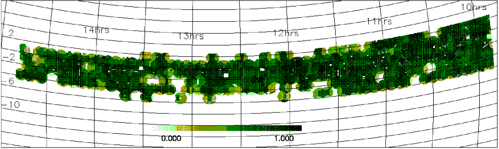
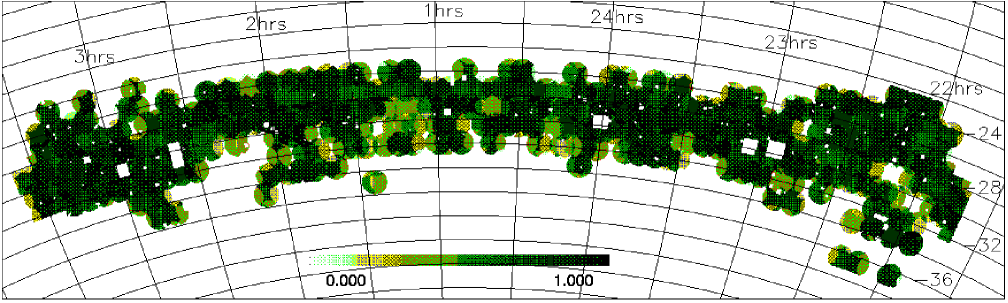
Figure 1: The sky coverage of the 2dFGRS dataset analysed in this paper. This dataset includes galaxy redshifts from all fields observed before  that have a redshift completeness greater than 70%. As the fields overlap and many are still to be observed, the completeness varies across the sky. The quantity represented by the grey-scale is the sector redshift completeness, $R({\mn@boldsymbol{\theta}})$, defined in Appendix A.

The 2dFGRS is selected in the photographic ${\rm b_{J}}$ band from the APM galaxy survey (Maddox et al. [1990b], [1990c], [1996]) and subsequent extensions to cit that include a region in the northern galactic cap ([2002]). The survey covers approximately 2151.6 deg² in two broad declination strips. The larger of these is centred on the South Galactic Pole (SGP) and approximately covers $-22^{\circ}\negthinspace.5$ $>$ $\delta$ $>$ $-37^{\circ}\negthinspace.5$, $21^{\rm h}40^{\rm m}$ $<$ $\alpha$ $<$ $3^{\rm h}40^{\rm m}$; the smaller strip is in the northern galactic cap and covers $2^{\circ}\negthinspace.5$ $>$ $\delta$ $>$ $-7^{\circ}\negthinspace.5$, $9^{\rm h}50^{\rm m}$ $<$ $\alpha$ $<$ $14^{\rm h}50^{\rm m}$. In addition, there are a number of pseudo-randomly located circular 2-degree fields scattered across the full extent of the low extinction regions of the southern APM galaxy survey. There are some gaps in the 2dFGRS sky coverage within these boundaries due to small regions that have been excluded around bright stars and satellite trails. The aim of the 2dFGRS is to measure the redshifts of all the galaxies within these boundaries with extinction-corrected ${\rm b_{J}}$ magnitudes brighter than 19.45. As described in Colless et al. ([2001]), this is attempted by dividing the target galaxies among a series of overlapping 2^o diameter fields. The degree of overlap of the fields is such that the number of targets assigned to each field is no greater than the 400 fibres that the 2dF instrument uses to obtain spectra for each target simultaneously. When all these 2^o fields have been observed, in early 2002, close to 250 000 galaxy redshifts will have been measured.

In this paper we use the 153 986 redshifts obtained prior to  in the main NGP and SGP strips. This sample covers a large fraction of the full 2dFGRS area, but as shown in Fig. 1, within this area the sampling rate varies with position on the sky. This is a direct consequence of some of the overlapping 2^o fields having not yet been observed and so is well understood and can be accurately modelled (see section 8 of Colless et al. [2001]).

For accurate statistical analysis of the 2dFGRS it is essential to understand fully the criteria that define its parent photometric galaxy catalogue and also the spatial and magnitude dependent completeness of the redshift survey. In the remainder of this section we describe the calibration and photometric accuracy of the parent galaxy catalogue. The accuracy and completeness of the redshift survey have been quantified in the survey paper Colless et al. ([2001]). Later, in Section 3, we complement the analysis of Colless et al. ([2001]) and our description of the 2dFGRS photometry by making a direct comparison with data from the overlapping Early Data Release (EDR) of the Sloan Digital Sky Survey (SDSS).

A detailed description of the calibration of the original APM catalogue can be found in Maddox et al. ([1990c] hereafter APMII). Here we start, in §2.1, by reviewing the important steps in this process, referring the reader to sections of APMII where many more details can be found along with various tests of the assumptions made in modelling the photometry. In §2.2, we describe the additional calibrating data and dust corrections that were used to define the input catalogue used to select objects for the 2dFGRS (see also [2002]). Finally, in §2.3, we describe how recently available CCD data and revised dust maps have been used to define the 2dFGRS magnitudes which were made public in the 100k release and which we adopt throughout this paper.

2.1 APM Photometric Calibration

The APM measures photographic density and for each image calculates the integrated density and area within an isodensity contour. If the images are not saturated, these are equivalent to an uncalibrated isophotal magnitude and corresponding isophotal area. These are converted to uncalibrated raw total magnitudes by modelling the intensity profile of each image as a gaussian. It is argued that this is a sufficiently accurate assumption as the observed profiles of the fainter galaxies are dominated by gaussian seeing, while the isophotal correction is small for the bright galaxies (APMII §2.1).

The isodensity threshold of the APM images corresponds roughly to a surface brightness of $25.0\,$mag arcsec^-2 (Shao et al. [2002]), but varies significantly within each UKST field. The main causes of this variation are geometric vignetting (variation of the effective area of the telescope with off axis angle) and desensitization of the hyper-sensitized photographic emulsion, which varies both systematically and randomly with field position (APMII §2.2). If the intrinsic sky brightness is uniform across the field of view then variations in the measured sky brightness can be used to estimate the variation of the sensitivity across the plate. In APMII §2.3, a model is developed to correct the raw total magnitudes using such maps of the measured sky brightness across each plate. This model assumes that the magnitudes being corrected are total magnitudes, that the true sky brightness is uniform across the field of view and that the UKST plates are of uniformly high quality. These corrections do not take account of saturation effects which are expected to become significant for galaxies brighter than ${\rm b_{J}}=16$ and may affect fainter high surface brightness ellipticals.

After applying the corrections described above the resulting field-corrected total magnitudes, $m_{\rm FC}$, are consistently defined over an individual UKST plate. However, the zeropoint and possibly the non-linearity can vary from plate to plate. Matched images on the substantial overlaps between the plates are used to find a set of transformations that bring the magnitudes on all the plates onto a common scale (APMII §3). Linear transformations of the form

$$m_{\rm A}=a_{i}+b_{i}m_{\rm FC}$$ (1)

were adopted to express the matched APM magnitudes, $m_{\rm A}$ in terms of the field-corrected magnitudes. Here, for plate $i$, $a_{i}$ is the zeropoint offset and $b_{i}$ a term that can correct for residual non-linearity. The degree of non-linearity in the original APM plates is quite small with an rms variation $\langle(b_{i}-1)^{2}\rangle^{1/2}=0.05$.

This procedure does not constrain the overall zeropoint or linearity of the survey. This global calibration was done using a limited number of ${\rm B}$ and ${\rm V}$-band CCD sequences that were spread reasonably uniformly across the survey area (APMII §4). Total CCD magnitudes were measured and converted into the ${\rm b_{J}}$-band using ${\rm b_{J}}={\rm B}-0.28({\rm B}-{\rm V})$ (Blair & Gilmore [1982]). Then a calibration curve of the form

$${\rm b_{J}}=a_{\rm global}+b_{\rm global}\,m_{\rm A}+c_{\rm global}\,m_{\rm A}^{2}$$ (2)

was determined by minimising the residuals between the final APM ${\rm b_{J}}$ and CCD total magnitude. A plot of the resulting calibration curve (both with and without the quadratic term) is shown in figure 1 of Maddox et al. ([1990a]). The CCD sequences were also used as a check of the zeropoints determined by plate matching (APMII §4.2).

It is important to realize that while the APM magnitudes are based on measurements which are approximately equivalent to an isophotal magnitude (with a somewhat uncertain and varying isophote), the APM correction and calibration procedure converts these into estimates of total magnitudes. The result should be that for galaxies in each interval of apparent magnitude the mean calibrated APM magnitude equals the mean total magnitude of the calibrating CCD data. The scatter about this mean relation is approximately $0.16$ magnitudes, this being driven mainly by the inaccuracy of photographic photometry, but also it is to be expected that within this scatter the residuals will correlate with surface brightness and possibly other properties of the galaxy images.

2.2 Calibration of 2dFGRS input catalogue

In 1994, when the input catalogue of the 2dFGRS was specified, substantially more CCD data was available than when the original APM catalogue was calibrated. Also new, improved plates and/or APM scans were available for a few UKST fields. Consequently both the plate matching and the final global calibration steps described above were redone using the new data. This time the parameters $b_{i}$ in equation (1) were kept fixed at unity. The reason for this was that in the original APM survey the deviations from linearity were quite small; also, for the purposes of selecting the ${\rm b_{J}}<19.45$ catalogue it was not necessary to have accurate bright magnitudes. The galaxies used in the plate matching were selected to have magnitudes in the range $19.5<{\rm b_{J}}<20.5$, close to the 2dFGRS magnitude limit.

The new CCD data was provided by Jon Loveday & Simon Lilly (private communication) and consists of 330 $10^{\prime}\times 10^{\prime}$ fields in ${\rm B}$ and ${\rm R}$ centred on galaxies selected from the Stromlo-APM catalogue (Loveday et al. [1996]). The data was taken using the CTIO 1.5m and total magnitudes were determined using using Sextractor ([1996]). The integration times were 2 minutes in ${\rm R}$ and 5 minutes in ${\rm B}$, leading to completeness limits of ${\rm B}\sim 21$ and ${\rm R}\sim 20$. This yields $13\,162$ images brighter than ${\rm b_{J}}=21$. Of these, $1\,760$ matched with galaxies in the APM data and these were used to determine the global calibration of APM magnitudes (i.e.  determine the parameters of equation 2). This new calibration was slightly different to the original APM calibration, both in terms of linearity correction and zero-point.

To accommodate an efficient observing strategy for the 2dFGRS it was necessary to extend the APM survey. Two overlapping strips of UKST plates in the region $9^{\rm h}<\alpha<15^{\rm h}$, $-7^{\circ}\negthinspace.5<\delta<3^{\circ}\negthinspace.5$, close to the NGP, were reduced using the standard APM galaxy survey procedures. For this area significant quantities of calibrating CCD data were not directly available. However, APM scans of the same UKST plates (reduced using a somewhat different suite of software) had been calibrated using CCD data by Raychaudhury et al. ([1994]). We had access to these calibrating catalogues, but not the original CCD data. We, therefore, set our global calibration by minimising the galaxy by galaxy residuals between our magnitudes and the calibrated magnitudes given by Raychaudhury et al. ([1994]).

The final step in the preparation of the magnitudes used to select the 2dFGRS parent catalogue was to apply extinction corrections. For this we used a new, high resolution dust map supplied to us by David Schlegel, in advance of the slightly modified map that was subsequently published in Schlegel, Finkbeiner & Davis ([1998]).

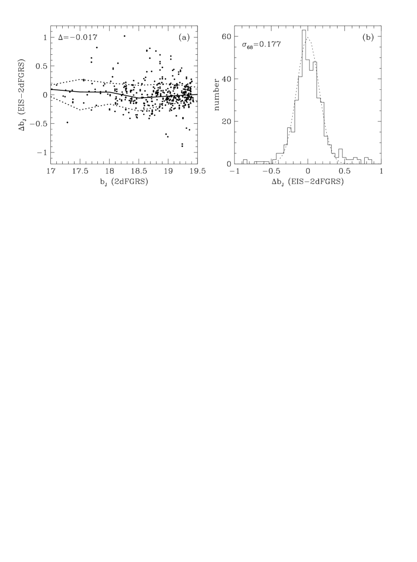
Figure 2: Comparison of 2dFGRS photographic ${\rm b_{J}}$ magnitudes with CCD magnitudes from EIS Patch B. Panel (a) is a scatter plot of the magnitude difference versus 2dFGRS magnitude and the solid and dotted lines show the magnitude dependence of the median, 16% and 84% quantiles of the distribution. The median magnitude difference, $\Delta$, for all the galaxies in the range $17<{\rm b_{J}}<19.5$ is indicated on the panel. The distribution of magnitude differences with respect to this median is shown as a histogram in panel (b). The dotted curve, which describes the core of this distribution quite well, is a gaussian with $\sigma=0.15$ magnitudes. A robust estimate of the width of this distribution, $\sigma_{68}$, defined such that $2\sigma_{68}$ spans 68% of the distribution, is also indicated on the panel.

2.3 100k 2dFGRS recalibration

Here we describe the improvements that were made to the 2dFGRS calibration and extinction corrections after target selection. These improved magnitudes (as well as the original magnitudes on which target selection was based) are available in the public 100k Release for the whole of the 2dFGRS parent catalogue. In outline, two main changes were made:

1. Corrections for plate-to-plate nonlinearities. The original calibrating CCD photometry concentrated on galaxies near ${\rm b_{J}}\simeq 20$, so the linearity of the photometry at bright magnitudes was hard to check. More recent CCD data showed that significant nonlinearities were sometimes present. The main tool used to correct these was the mean optical to infrared colour on each plate between 2dFGRS and the 2MASS survey.

2. Improved estimates of the foreground extinction. The original 2dFGRS selection, performed in 1994, was based on magnitudes corrected using a preliminary version of the Schlegel et al. ([1998]) dust map. The final version and calibration of this map differed slightly from the one originally adopted. On average, the updated extinction corrections are larger than those initially adopted, by a factor of approximately 1.3. This yields rms shifts in zero point of 0.02 magnitudes in the NGP, and half this in the SGP.

In principle, variations in plate-to-plate nonlinearity might not be expected to be a problem. These effects can be diagnosed when the magnitudes in the overlap region between two different plates are compared. The ideal case would then be a set of plates with a consistent set of magnitudes in the overlaps, whose absolute zero point and degree of linearity can be assessed by combining all the calibrating CCD photometry. The practical difficulty is that the number of bright galaxies for comparison in the overlaps can be small where one of the plates is of lower quality, preventing an accurate determination of the linearity of that plate. This turns out to have been a significant problem in the NGP zone, where we used fewer plates than in the SGP, and where the quality was less homogeneous. Nevertheless, there were some nonlinearity problems in the SGP also.

The direct measurement of plate nonlinearities requires large CCD datasets. In the SGP, we were able to make comparison with the results of the public ESO Imaging Survey (EIS) in the Patch B region (Prandoni et al. [1999]) and the Chandra Deep Field (Arnouts et al. [2001]). We also had access to data from the ESO–Sculptor Survey (Arnouts et al. [1997]). The Patch B dataset is the largest, and showed the 2dFGRS photometry to be consistent with linear in this plate (UKST 411); there was significant nonlinearity in the Chandra Deep Field (UKST 418), however. The EIS datasets have accurately determined colour equations, so we are able to make an accurate determination of the colour equation between ${\rm b_{J}}$ and Johnson B & V:

$${\rm b_{J}}={\rm B}-(0.267\pm 0.019)({\rm B}-{\rm V}),$$ (3)

verifying our standard colour term of 0.28.

In the north, the main comparison was with the MGC survey ([2002]). This covers a $36\,$deg² strip between $10^{\rm h}<\alpha<15^{\rm h}$ and overlaps with 15 UKST plates in the 2dFGRS NGP strip (a total of 5205 galaxies in common). Data are available only in a blue filter (${\rm B}_{\rm MGC}$) that differs somewhat from the 2dFGRS ${\rm b_{J}}$. The MGC thus cannot yield an absolute calibration for 2dFGRS, but the accuracy of the data (a limiting magnitude of ${\rm B}_{\rm MGC}\simeq 24$) means that precise measures of nonlinearity and relative zero-points were possible. For each UKST plate, we fitted a linear relation of the form

$${\rm B}_{\rm MGC}=a_{i}+b_{i}{\rm b_{J}},$$ (4)

where ${\rm b_{J}}$ is the observed 2dFGRS magnitude, prior to dust correction. In this way we determined the non-linearity $b_{i}$ and relative zeropoint $a_{i}$ of each of the 15 UKST plates. Nonlinearities of up to $|{\rm b}_{i}-1|=0.2$ were measured (median 0.08). That variations in linearity exist in the NGP strip is not surprising. As discussed in APMII §2.3, the model that was constructed to correct the raw APM magnitudes for vignetting and variations in plate sensitivity assumes that the UKST plates are of uniform quality. In particular, it is assumed that the sky brightness varies by only a small amount both across the field of view of each plate and from one plate to another. This assumption is less valid for the NGP strip, as the UKST plates used here were less homogeneous than in the original APM survey.

Based on these results, nonlinearities must also exist for plates where large CCD datasets are lacking. In the absence of this information, we resorted to the only uniform all-sky source of digital galaxy photometry: the near-infrared 2-Micron All-Sky Survey ([2000]). In particular, we concentrated on the ${\rm J}$-band 2MASS magnitudes for 2MASS-detected galaxies that are also in the 2dFGRS. Although the 2MASS data are at a much longer wavelength than the APM photometry, nevertheless comparing 2MASS and APM photometry proved to be very useful. The plate matching procedure used to define the 2dFGRS magnitudes should be accurate at approximately ${\rm b_{J}}=20$ (the typical magnitude of most of the galaxies used in the matching), and this is verified by our original calibrating CCD photometry. However, residual non-linearity can result in significant plate-to-plate offsets at bright magnitudes. As the median magnitude of the matched 2MASS–2dFGRS galaxies is ${\rm b_{J}}\simeq 17.5$, such offsets manifest themselves as variations in the median ${\rm b_{J}}-{\rm J}$ of the matched galaxies. For this comparison, we used magnitudes corrected for extinction using the most recent dust maps. Any offset ($\Delta_{\rm 2MASS}$) in this median colour over a single UKST plate with respect to the global average should thus indicate an error in the bright 2dFGRS magnitudes, and hence a nonlinearity. We were able to verify that this assumption worked well by comparison with the 18 plates with direct nonlinearity measurements, and we therefore assumed that measurements of $\Delta_{\rm 2MASS}$ could be used to diagnose nonlinearities in all plates. In practice, rather than assuming that plate overlaps assured an exact matching at some specific magnitude between 20 and 21, an empirical approach was taken. The MGC data showed that both nonlinearity and the relative zero-point offsets at 19.45 correlated with $\Delta_{\rm 2MASS}$, so a single value for $\Delta_{\rm 2MASS}$ was used to give an estimate for each of these quantities.

The practical problem with this strategy is that not all plates have an accurate measurement of $\Delta_{\rm 2MASS}$. The dispersion in ${\rm b_{J}}-{\rm J}$ is approximately 0.5 magnitudes, so several hundred 2MASS galaxies per plate are required to give a sufficiently accurate measurement of the offset. Some plates fail to satisfy this criterion, since the full 2MASS survey is not yet available. We therefore proceeded as follows. Examining the trend of $\Delta_{\rm 2MASS}$ with sky position showed strong evidence for an approximately linear variation of $\Delta_{\rm 2MASS}$ with RA and declination in both NGP and SGP. It is quite understandable that the plate-matching could allow a slow drift of the magnitude linearity in this way; we therefore used a linear fit as the initial estimate of $\Delta_{\rm 2MASS}$, and hence nonlinearity, in any given plate. Where the measurement of $\Delta_{\rm 2MASS}$ was significantly different from the position-dependent fit, a Bayesian approach was adopted, as follows. Consider the deviation of the exact value of $\Delta_{\rm 2MASS}$ with respect to the fit – call this $d_{\rm t}$, and let it have a prior probability distribution $P(d_{\rm t})$. We have an estimate of $d_{\rm t}$ from the limited 2MASS data that actually exist – call this $d_{2\rm m}$. We are interested in the probability of $d_{t}$ given $d_{2\rm m}$, for which Bayes’ theorem says

$$P(d_{\rm t}|d_{2\rm m})\propto P(d_{\rm t})P(d_{2\rm m}|d_{\rm t}).$$ (5)

This probability can be maximized to give a preferred value of $d_{\rm t}$ for a given $d_{2\rm m}$, taking into account the known statistical errors on $d_{2\rm m}$. An estimate of the prior $P(d_{\rm t})$ was obtained from the plates with very accurate values of $d_{2\rm m}$ and/or those with CCD data. This procedure allows us to interpolate smoothly between accepting $\Delta_{\rm 2MASS}$ where it is well defined, and using the position-dependent fit where the 2MASS data are sparse on an individual plate. This yields a best estimate of $\Delta_{\rm 2MASS}$ for each plate, and hence an estimate of the linearity of the initial 2dFGRS photometry on that plate. Of course, direct measurements of nonlinearity from CCD data are to be preferred where they exist, and the direct results from the MGC and EIS comparisons were used to recalibrate the relevant plates, without reference to the 2MASS results.

Thus for the magnitudes given in the 100k release the use of 2MASS and MGC data has augmented the matching of plates that was done using the overlaps. In the SGP the corrections to the magnitudes are modest. The rms variation in linearity is $\langle(b-1)^{2}\rangle^{1/2}=0.034$ and the rms shift of the zeropoint at ${\rm b_{J}}=19.45$ is $0.043$ magnitudes. In the NGP, which was constructed from a less homogeneous set of UKST plates, the changes are much more significant: the rms variation in linearity is $\langle(b-1)^{2}\rangle^{1/2}=0.106$ and the induced rms shift of the zeropoint at ${\rm b_{J}}=19.45$ is $0.123$ magnitudes.

After applying these nonlinear transformations, the corrected magnitudes should now be on a consistent scale on all plates in both SGP and NGP. The overall zeropoint will still be that set at the faint end by our initial CCD calibration. As an external absolute check of the zeropoint, we compared with the optical CCD data from the EIS Patch B (Prandoni et al. [1999]), the EIS Chandra Deep Field (Arnouts et al. [2001]), and the ESO-Sculptor survey (Arnouts et al. [1997]), since these are the largest datasets, and have the best characterized colour equations. The mean offset of these three fields with respect to the original APM magnitudes was $0.03$ magnitudes, in the sense that the original magnitudes were too faint. This shift was applied, placing our magnitudes on average on the same zeropoint as the EIS. The standard deviation of the three offsets was $0.035$ magnitudes, which is in fact smaller than the $0.07$ plate-to-plate dispersion that we would expect over a large sample. Therefore, it is conservative to assume that the rms uncertainty in the 2dFGRS overall zeropoint is $0.07/\sqrt{3}=0.04$ magnitudes, assuming no error in EIS. The internal tests of Prandoni et al. ([1999]) suggest that any systematic errors in the EIS calibration are smaller than this figure. The EIS and calibrated 2dFGRS magnitudes are compared in Fig. 2. The rms error in an individual galaxy magnitude is approximately 0.15. The effect of these recalibrations, and the change in the dust correction, is shown in figures 13 and 14 of Colless et al. ([2001]).

3 Comparison with the SDSS

Here we complement the description given above and in the survey construction papers ([2001, 2002]) by making a direct comparison of the 2dFGRS catalogue with the Early Data Release (EDR) of the Sloan Digital Sky Survey (SDSS). The two datasets have approximately 30 000 galaxies in common of which about 10 000 have redshift measurements in both surveys. Here we use these data to assess the accuracy of the 2dFGRS photometry, the completeness of the parent galaxy catalogue and the accuracy and reliability of the redshifts.

3.1 Photometric Accuracy

The 2dFGRS magnitudes that we use here are the same as those made public in our June 2001 100k Release. As described in §2, they are pseudo-total magnitudes measured from APM scans of photographic plates from the UK Schmidt Telescope (UKST) Southern Sky Survey and their precision depends on the accuracy of the zeropoint, and non-linearity corrections of each plate, as well as the measurement errors within each plate. The overlap of SDSS and 2dFGRS is in the NGP where our calibration corrections were largest and so the comparison provides a strong test of these calibrations. Note that in the comparisons made in this section we apply extinction corrections to both the 2dFGRS and SDSS data based on the extinction map of Schlegel et al. ([1998]).

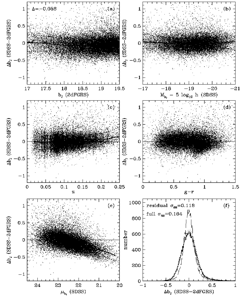
Figure 3: Comparison of 2dFGRS photographic ${\rm b_{J}}$ magnitudes and CCD magnitudes from SDSS. Panel (a) is a scatter plot of the magnitude difference versus 2dFGRS apparent magnitude and the solid and dotted lines show the magnitude dependence of the median, 16% and 84% quantiles of the distribution. The median magnitude difference, $\Delta$, for all the galaxies in the range $17<{\rm b_{J}}<19.5$ is indicated on the panel. The following four panels show the SDSS-2dFGRS magnitude differences versus (b) absolute magnitude, (c) redshift, (d) ${\rm g}-{\rm r}$ colour and (e) surface brightness. The surface brightness is the SDSS measurement of mean surface brightness within the Petrosian half light radius converted into the ${\rm b_{J}}$ band. In all these panels we again show the 16%, 50% and 84% quantiles of the distribution. In all but panel (a), the residual is calculated after subtracting the median offset from each UKST plate. The distribution of magnitude differences with respect to the median is shown as a histogram in panel (f). The dotted curve, which describes the core of this distribution quite well, is a gaussian with $\sigma=0.15$ magnitudes. A robust estimate of the width of this distribution is $\sigma_{68}=0.164$, where $\pm\sigma_{68}$ spans 68% of the distribution. The empirical model we adopt to describe the full 2dFGRS magnitude measurement errors is shown by the smooth solid curve in panel (f) (see text for details). The dashed curve in (f), which has $\sigma_{68}=0.118$, is the distribution of residual magnitude difference relative to the mean correlation of residual with surface brightness shown in panel (e).

The panels of Fig. 3 compare 2dFGRS magnitudes with Petrosian CCD magnitudes from the SDSS EDR ([2002]). The definition of the SDSS Petrosian magnitudes is described in Blanton et al. ([2001]), which also demonstrates they are essentially equivalent to total magnitudes for disk galaxies while underestimating the luminosity of spheroids by approximately 0.15 magnitudes. This is very similar to the behaviour of the total magnitudes derived using Sextractor ([1996]), which were used in the APM and 2dF calibration. We note that for the purposes of calibration the less robust SDSS model magnitudes (the default magnitudes in the SDSS database) are not suitable. Here we have estimated ${\rm b_{J}}$ from the SDSS photometry using the transformation

$${\rm b_{J}}={\rm g}+0.155+0.152\,({\rm g}-{\rm r}).$$ (6)

This relation comes from adopting the colour equations given for $B$ and $V$ in Fukugita et al. ([1996]) and combining these with ${\rm b_{J}}=B-0.28(B-V)$ (Blair & Gilmore [1982]), as verified by the EIS data. Fig. 3d is an empirical test of the colour term in our adopted transformation. The very weak dependence of the median magnitude difference on colour is consistent with the $0.152({\rm g}-{\rm r})$ colour term. A simple least squares fit gives a coefficient $0.152\pm 0.004$ and so is strongly inconsistent with the colour term of $0.088({\rm g}-{\rm r})$ that was adopted by Blanton et al. ([2001]) in the comparison between the SDSS and the 2dFGRS luminosity function ([1999]).

Fig. 3a shows that, in the range $17<{\rm b_{J}}<19.5$, the relation between 2dFGRS and SDSS Petrosian magnitudes is close to linear and that the scatter between the two measurements is only weakly dependent on apparent magnitude, being slightly greater at brighter magnitudes. There is evidence for a very weak departure from linearity with $\Delta{\rm b_{J}}^{\rm SDSS}\approx 0.94\Delta{\rm b_{J}}^{\rm 2dF}$ for ${\rm b_{J}}<18$, but at fainter magnitudes, where the vast majority of 2dFGRS galaxies lie, the relation is accurately linear. There is a zeropoint offset, with the median 2dFGRS magnitude being fainter than that of the SDSS by $|\Delta|=0.058$ magnitudes. This is not surprising as the zeropoint in the SDSS EDR data is only claimed to be accurate to $\pm 0.03$ magnitudes ([2001]) and similarly we estimate the accuracy of the 2dFGRS zeropoint to be $\pm 0.04$ magnitudes (see Section 2.3). The SDSS EDR data span 15 UKST plates in the NGP region of the 2dFGRS and there is some plate-to-plate variation in the median offset between 2dFGRS and SDSS Petrosian magnitudes. We find an rms variation of $0.083$ magnitudes which is in reasonable agreement with the 0.07 magnitudes rms we estimated from the calibrating photometry, and adds little to the measurement error in an individual galaxy magnitude. We expect the variation in plate zeropoints to be somewhat less in the SGP region of the 2dFGRS as this region was constructed from a more homogeneous set of high quality UKST plates than is available in the NGP. At present there are not enough public CCD data to verify this claim. In the other panels of Fig. 3 the median offset between 2dFGRS and SDSS magnitudes on each plate has been subtracted from the magnitude differences.

Figs. 3b and c show, for the subset of galaxies for which redshifts have been measured, the magnitude difference as a function of absolute magnitude and redshift. Fig. 3b indicates that the median offset between 2dFGRS and SDSS magnitudes is, to a good approximation, independent of absolute magnitude. In Fig. 3c below $z\approx 0.16$ there is very little variation in the median magnitude difference. At higher redshift there is a weak trend with the 2dFGRS ${\rm b_{J}}$-band magnitude becoming systematically brighter than that inferred from the SDSS. We note that, in contrast, the isophotal magnitudes used by Blanton et al. ([2001]) in attempting to reproduce the 2dFGRS LF of Folkes et al. ([1999]), which they argued were a good approximation of APM magnitudes, falsely predicted that the 2dFGRS magnitude would monotonically become fainter than the SDSS magnitude with increasing redshift. The main reason for the inaccuracy of the Blanton et al. ([2001]) model is that it neglected to take account of the way in which APM and 2dFGRS magnitudes are calibrated. We recall that the calibration of the raw APM magnitudes involves both a zeropoint and a non-linearity correction so that, in principle, for galaxies in each interval of apparent magnitude the median calibrated 2dFGRS magnitude equals the median total magnitude of the calibrating CCD data ([1990c]). The weak variation with redshift seen in Fig. 3c is, in fact, probably due to systematic variation with redshift of the relationship between ${\rm g}$, ${\rm r}$ and ${\rm b_{J}}$ magnitudes. The colour equation we have adopted is empirically verified to be accurate for the bulk of the 2dFGRS galaxies, which have a median redshift of $z\approx 0.1$. At higher redshift, as different rest frame spectral features pass through the three filter bands, one expects small changes in the colour equation.

In Fig. 3e we see that there is a significant correlation between the SDSS-2dFGRS magnitude residual and surface brightness. The 2dFGRS magnitudes of galaxies with surface brightnesses of $\mu_{{\rm b_{J}}}\approx 23$ mag arcsec^-2 are correct in the mean, but the magnitudes of higher surface brightness galaxies become progressively too faint. A similar correlation is also found by Cross et al. ([2002b]) when comparing 2dFGRS and MGC photometry. Such a correlation is to be expected due to saturation of the UKST plates ([1995]). This variation of measured magnitude with surface brightness does contribute significantly to the overall 2dFGRS magnitude measurement error. The distribution shown by the dashed curve in Fig. 3f shows that correcting for the variation with surface brightness would reduce the width of the error distribution from $\sigma_{68}=0.164$ to $\sigma_{68}=0.118$ magnitudes. However, for the full 2dFGRS dataset this cannot be done as there is not yet a sufficiently accurate measure of surface brightness (but see Shao et al. [2002]). The surface brightness correlation makes negligible difference to the overall luminosity function and 2dFGRS selection function. Here all one needs is an accurate model of the overall distribution of the 2dFGRS magnitude measurement errors. However if the luminosity function is derived for subsamples split by spectral type (or another parameter that correlates with surface brightness) small corrections have to be made ([2002]).

The histogram in Fig. 3f shows the distribution of SDSS-2dFGRS magnitude differences. The dotted curve which describes the core of the distribution quite well is a gaussian with $\sigma=0.15$. The tail, in excess of this gaussian, of objects for which the 2dFGRS measures a fainter magnitude than the SDSS is very small. There is a somewhat larger tail of objects for which the 2dFGRS measures a brighter magnitude than the SDSS. It is most likely that these objects are close pairs of images which the SDSS has resolved, but which are merged into a single object in the 2dFGRS catalogue. This is precisely what is found for the 2dFGRS when compared to the MGC catalogue ([2002]) by Cross et al. ([2002b]). The overall distribution of magnitude differences is well fitted by the model shown by the solid curve. This model is the sum of a gaussian and a log-normal distribution. The gaussian component has $\sigma=0.14$ and accounts for 70% of the probability and the remaining 30% is distributed as a gaussian in $\ln(1+\Delta{\rm b_{J}})$ with $\sigma=0.235$. We adopt this model as an empirical description of the distribution of the 2dFGRS magnitude measurement errors. In so doing, we are assuming that the random measurement errors in the SDSS CCD Petrosian magnitudes do not contribute significantly to the width of this distribution. This assumption is consistent with the comparison of the SDSS photometry with the deeper MGC CCD photometry in Cross et al. ([2002b]).

3.2 Completeness of the 2dF Parent Catalogue

Figure 4: In the upper panel the solid histogram shows, as a function of apparent magnitude, the percentage of photometrically classified galaxies in the SDSS EDR that have 2dFGRS counterparts. This estimate of the completeness should be ignored rightwards of the vertical dashed line at ${\rm b_{J}}=19.0$. Fainter than this galaxies are absent from the 2dFGRS catalogue simply due to the faint magnitude limit of the catalogue which varies from $19.2<{\rm b_{J}}<19.5$. The horizontal line indicates our adopted 91% completeness. The dotted histogram shows the percentage of spectroscopically confirmed SDSS galaxies that have 2dFGRS counterparts. The dashed histogram shows the percentage of objects in the 2dFGRS parent catalogue in the same area that are spectroscopically identified as stars. The lower panel shows the completeness as a function of the mean galaxy surface brightness within the Petrosian half light radius. In this estimate only galaxies in the magnitude range $17.0<{\rm b_{J}}<19.0$ are considered. Again we show estimates relative to the SDSS parent photometric catalogue (solid histogram) and the spectroscopically confirmed galaxies (dotted histogram). The solid curve shows, on an arbitrary scale, the distribution of surface brightnesses for the $11\,171$ galaxies in the SDSS sample in this same magnitude range.

In constructing the parent catalogue of the 2dFGRS the same parameters and thresholds were used to perform star-galaxy separation as in the original APM galaxy survey ([1990b]). Thus, the expectation is that the parent galaxy catalogue will be 90-95% complete and contamination from stellar objects will be 5-10% ([1990b]). In fact, the spectroscopic identification of the 2dFGRS objects shows that the stellar contamination is 5.4% overall and only very weakly dependent on apparent magnitude (see Fig. 4). The SDSS EDR allows us to make a useful test of the 2dFGRS galaxy completeness. In the SDSS commissioning data the star-galaxy classification procedure is expected to be better than 99% complete and have less than 1% stellar contamination ([2001]). In Fig. 4 we assess the completeness of the 2dFGRS parent catalogue both against the SDSS photometric galaxy catalogue and against the SDSS sample of spectroscopically confirmed galaxies.

To compare to the SDSS spectroscopic sample we selected the 13 290 SDSS objects that are spectroscopically confirmed as galaxies and have magnitudes brighter than ${\rm b_{J}}=19.5$. For the SDSS photometric galaxy catalogue we used the 16 371 objects brighter than ${\rm b_{J}}=19.5$ that are flagged in the EDR database as being members of the SDSS main galaxy survey. The solid (dotted) histogram in the upper panel of Fig. 4 shows, as a function of apparent magnitude, the percentage of the photometrically classified (spectroscopically confirmed) galaxies that have counterparts in the 2dFGRS. The completeness estimates vary very little with magnitude over the entire range $16<{\rm b_{J}}<19.0$. The dip evident in the faintest bins is an artifact. Because of random measurement errors in the APM/2dFGRS magnitudes and because the magnitude limit in some parts of the NGP strip is as bright as ${\rm b_{J}}\approx 19.2$ (see [2001] figures 13 and 14), some of the selected SDSS galaxies have APM magnitudes that are too faint to be included in the 2dFGRS parent catalogue. Over the magnitude range $17.0<{\rm b_{J}}<19.0$ the completeness relative to SDSS photometric galaxy catalogue is between 88.5% and 92%, while the completeness measured relative to the spectroscopically confirmed SDSS galaxy catalogue is slightly higher at 91% to 95%.

The lower panel of Fig. 4 shows the completeness as a function of the mean galaxy surface brightness within the Petrosian half light radius. The surface brightness is estimated from the extinction-corrected SDSS g and r band data and expressed in the ${\rm b_{J}}$ band using the relation given in equation (6). In this estimate only galaxies in the magnitude range $17.0<{\rm b_{J}}<19.0$ are considered. Also shown in this figure is the surface brightness distribution for galaxies in this magnitude range. At both extremes of surface brightness the completeness of the 2dFGRS galaxy catalogue diminishes. At the faint end this is because the galaxies become to faint to reliably detect, while at the bright end a fraction are mis-classified as stars. However over most of surface brightness range populated by galaxies the completeness of the 2dFGRS is uniformly high. Relative to the SDSS catalogue of photometrically classified galaxies the completeness has a broad peak of 93.4% for $21.8<\mu_{{\rm b_{J}}}<23.2$, while averaged over the complete galaxy surface brightness distribution the completeness is 90.9%. Thus, while the incompleteness of the 2dFGRS catalogue is approximately 9%, only 2.5% incompleteness is dependent on the galaxy surface brightness, with only one third of this coming from losses at the low surface brightness end. The dominant reason for the approximately 9% incompleteness in the 2dFGRS galaxy catalogue appears to be due to mis-classification of images. This conclusion has also been reached more directly by Pimbblet et al. ([2001]), and Cross et al. ([2002b]) by comparing the 2dFGRS parent catalogue with deeper wide-area CCD photometry. See also Caretta et al. ([1993]), but note the APM catalogue they analyzed was APMCAT (http://www.ast.cam.ac.uk/$\tilde{\hphantom{i}}$apmcat; Irwin et al. [1994]; Lewis & Irwin [1996]) which although based on the same scan data as the Maddox et al. ([1990b]) APM galaxy catalogue has a different algorithm for star-galaxy classification and less reliable galaxy photometry. They have shown that while the 2dFGRS misses some low surface brightness galaxies more are lost due to mis-classification, particularly of close galaxy and galaxy-star pairs.

The mis-classification of some close galaxy pairs could also explain the slight difference we have found between the completeness measured relative to the SDSS spectroscopically confirmed and photometrically classified galaxy catalogues. Assuming the SDSS spectroscopic sample is a random sample of the photometric sample, then apart from the effect of the very small fraction ($<$1%) of photometrically classified galaxies which turn out to be stars or artifacts of some kind, we would expect the two estimates of incompleteness to agree. However, the spectroscopic sample is not a random sample as close pairs of galaxies are under-represented because of the mechanical limits on how close the optical fibres that feed the spectrograph can be placed. This is a plausible explanation of the difference between the two completeness estimates. We therefore adopt $91\pm 2$% as the 2dFGRS galaxy completeness, consistent with the estimate from the SDSS photometric catalogue. This value is indicated by the horizontal line in the upper panel of Fig. 4.

3.3 Accuracy and Reliability of Redshift Measurements

Figure 5: A histogram of the 2dFGRS-SDSS redshift differences for a sample of 10 763 galaxies for which both surveys have measured redshifts with $z>0.003$. The smooth curve is a gaussian with $\sigma=85.0\,{\rm km\,s^{-1}}$.

The 2dFGRS redshift measurements are all assigned a quality flag $Q$ ([2001]). For most purposes only $Q\geq 3$ redshifts are used. From a comparison of repeat observations, Colless et al. ([2001]) estimated that these have a reliability (defined as the percentage of galaxies whose redshifts are within a $600\,{\rm km\,s^{-1}}$ tolerance) of 98.4% and an rms accuracy of $85\,{\rm km\,s^{-1}}$. For higher quality spectra, $Q\geq 4$, these figures improve to $>99$% and less than $60\,{\rm km\,s^{-1}}$, respectively. Comparison of the 2dFGRS redshifts with the 10 763 galaxies which also have redshift measurements in the SDSS EDR provides a useful check of these numbers. The fraction of objects for which the redshifts differ by more than $600\,{\rm km\,s^{-1}}$ is only 1.0% and this presumably includes some cases where it is the SDSS redshift that is in error. The redshift differences for the remainder are shown in Fig. 5. This distribution has a width of $\sigma_{68}=85.0\,{\rm km\,s^{-1}}$ (defined so that $2\sigma_{68}$ spans 68% of the distribution). Taking account of the contribution from the rms error in the SDSS measurements this implies a smaller redshift error than the estimate of Colless et al. ([2001]). Part of the reason for the difference in these figures is that the SDSS galaxies are on average brighter than typical 2dFGRS galaxies. Also we have only compared measurements when both the SDSS and 2dFGRS redshifts are greater than $0.003$. This excludes a small number of 2dFGRS redshifts that are very small due either to contamination of the spectra by moonlight or light from a nearby star. If we further reduce the sample to 10 022 (or 8 059) objects by excluding objects whose SDSS and 2dFGRS positions differ by more than 1 (or 0.5) arc second then the reliability increases slightly to 99.14 (or 99.22%). This could indicate that some of the discrepant redshifts arise from very close galaxy pairs that are unresolved in the 2dFGRS parent catalogue.

4 k+e corrections

Figure 6: Galaxy ${\rm g}-{\rm r}$ colours as a function of redshift. The symbols and error bars show, for each 2dFGRS spectral type, the median, $10$ and $90$ centiles of the ${\rm g}-{\rm r}$ colour distribution, as a function of redshift. The curves are the predictions for model galaxies, computed using the Bruzual & Charlot stellar population synthesis code, whose star formation histories have been selected to reproduce, as closely as possible, the median colour as a function of redshift in each class.

The final ingredient that is required to characterise the selection function of the 2dFGRS is a model describing the change in galaxy magnitude due to redshifting of the galaxy spectra relative to the ${\rm b_{J}}$-filter bandpass (k-correction) and galaxy evolution (e-correction). These corrections depend on the galaxy’s spectrum and star formation history. As these are correlated, one can parameterize the k+e corrections as functions of the observed spectra.

A subset of 2dFGRS spectra have been classified using a method based on Principal Component Analysis (PCA). A continuous parameter, $\eta$, is defined as a linear combination of the first two principal components ([2002]). The definition of $\eta$ is such that its value correlates with the strength of absorption/emission features. Galaxies with old stellar populations and strong absorption features have negative values of $\eta$, while galaxies with young stellar populations and strong emission lines have positive values. Therefore, we expect the value of $\eta$ to correlate with the galaxy’s k and k+e correction. In Madgwick et al. ([2002]), the continuous $\eta$ distribution was divided into four galaxy classes (Type 1: $\eta<-1.4$, Type 2: $-1.4\leq\eta<1.1$, Type 3: $1.1\leq\eta<3.5$, Type 4: $3.5\leq\eta$) and the mean k-correction for each type was estimated from the mean spectra of galaxies in each class. A current weakness of this approach is that the overall system response of the 2dF instrument is not well calibrated. This implies that the resulting k-corrections have a systematic uncertainty of around 10% ([2002]). Due to this problem and also because we wish to estimate k+e corrections and not just k-corrections, we have taken a complementary approach.

Figure 7: Model k and k+e corrections for each 2dFGRS spectral type. The symbols in the top panel show the k-corrections for four models selected to match the ${\rm g}-{\rm r}$ colours as a function of redshift plotted in Fig. 6. The curves show the corresponding k-corrections adopted in Madgwick et al. (2002). The symbols in the lower panel show our model k+e corrections. In this case, the smooth curves are simple analytic fits [Type 1 : $k+e=(2z+2.8z^{2})/(1+3.8z^{3})$, Type 2: $k+e=(0.6z+2.8z^{2})/(1+19.6z^{3})$, Type 3: $k+e=(z+3.6z^{2})/(1+16.6z^{3})$, Type 4: $k+e=(1.6z+3.2z^{2})/(1+14.6z^{3})$].

The spectrum of any individual galaxy will evolve with time as its star formation rate changes and its stellar population evolves. Consequently, the spectral type of such a galaxy could vary with cosmic time. Therefore, if we want to group the observed galaxies into discrete classes so that the evolution of each class can be described by a single model, we should bin the galaxies in both $\eta$ and $z$. Instead, we will bin the galaxies only in $\eta$ and so not explicitly take account of galaxies which evolve from one spectral class to another. We do this as adopting a more complicated model makes little difference to our results and also it enables us to compare our k-corrections directly with those used in Madgwick et al. ([2002]).

In Fig. 6, we plot the median observed ${\rm g}-{\rm r}$ colour measured from the SDSS EDR data as a function of redshift for each spectral class determined from the 2dFGRS spectra. As expected, we see that galaxy colour and its dependence on redshift correlates with the spectral class. Type 1 galaxies, with the most negative value of $\eta$ and oldest stellar populations, are reddest and Type 4 are bluest. The curves plotted on Fig. 6 are models constructed using the Bruzual & Charlot ([1993]; in preparation, see also Liu, Charlot & Graham [1993] and Charlot & Longhetti [2001]) stellar population synthesis code. In a manner very similar to that described by Cole et al. ([2001]), we ran a grid of models each with the same fixed metallicity ($Z=Z_{\odot}/2$) and with a star formation history of the form $\psi(t)\propto\exp(-[t(z)-t(z_{\rm f})]/\tau)$, with a set of different timescales, $\tau$. Here, $t(z)$ is the age of the universe at redshift $z$ and the galaxy is assumed to start forming stars at $z_{\rm f}=20$. To relate redshift to time, we have assumed a cosmological model with $\Omega_{0}=0.3$, $\Lambda_{0}=0.7$ and Hubble constant $H_{0}=70\,{\rm km\,s^{-1}}$ Mpc^-1. The k and k+e corrections that we derive are only very weakly dependent on these choices.

The models plotted Fig. 6 are the four which best reproduce the observed dependence of the ${\rm g}-{\rm r}$ colours with redshift for the four spectral types. They have $\tau=1,5,15$ and $1000$ Gyr for Type 1,2,3 and 4 respectively. The models provide a complete description of the galaxy spectral energy distribution and its evolution and so can be used to define k or k+e corrections for each spectral type. These are shown by the symbols in Fig. 7. The Madgwick et al. ([2002]) k-corrections, shown by the curves in the top panel, are similar but systematically smaller than those we have derived. This systematic difference is comparable to the systematic difference expected given the current uncertainty in the calibration of the 2dF instrument, upon which the Madgwick et al. ([2002]) k-corrections rely. The bottom panel of Fig. 7 shows our k+e corrections. Simple analytic fits to the k+e correction for each spectral class are given in the figure caption and shown by the smooth curves. Note that the ordering of the k and k+e corrections is not the same. This is because there are competing effects that contribute to the evolutionary correction. As the redshift increases, the age of the stellar population viewed decreases. This effect makes galaxies brighter with increasing redshift, since younger stellar populations have smaller mass-to-light ratios, and also changes the shape of the galaxy spectrum. However, there are fewer stars present at earlier times and this tends to produce a decrease in luminosity with redshift. For galaxies with ongoing star formation (Types 2,3 and 4) these effects can all be significant in determining the overall k+e correction.

Figure 8: The curves show the fits, $k(z)=(2.2z+6z^{2})/(1+15z^{3})$ and $k(z)+e(z)=(z+6z^{2})/(1+20z^{3})$, to the mean k and k+e correction as a function of redshift. The mean corrections at each redshift, shown by the symbols, have been computed as a function of redshift from the known fractions of each spectral type. The error bars show the rms scatter about the mean of these distributions.

It is not possible to assign values of $\eta$ to all the galaxies in the 2dFGRS. In fact, only galaxies with $z<0.2$ are classified in this way and approximately 5% of these have spectra with insufficient signal-to-noise to define $\eta$. Thus, for some purposes it is necessary to adopt a mean k or k+e correction that can be applied to all galaxies in the survey. In Fig. 8 we show k and k+e corrections averaged over the varying mix of galaxies at each redshift and give simple fitting formulae. We recall that our estimate of the evolutionary correction assumes a cosmological model with $\Omega_{0}=0.3$, $\Lambda_{0}=0.7$ and $H_{0}=70$km  s^-1 Mpc^-1 in order to relate redshift and look back time. When estimating the galaxy luminosity function for cosmological models with different parameters we retain the same k+e corrections rather than recomputing the best fitting Bruzual & Charlot model. While not being entirely consistent, in practice this makes very little difference to our luminosity function estimates. In section 8.1, we constrain the uncertainty in k+e correction by comparing luminosity functions estimated in different redshift bins. This enables us to assess the contribution to the error in the luminosity function estimates arising from uncertainties in the k+e corrections.

5 Mock and Random Catalogues

One of the main purposes of deriving a quantitative description of the survey selection function is to make it possible to construct random (unclustered) and mock (clustered) galaxy catalogues. The random catalogues provide a very flexible description of the selection function and are most often employed when making estimates of galaxy clustering. The mock catalogues, where the galaxy positions are determined from cosmological N-body simulations, are even more useful. The underlying galaxy clustering and galaxy luminosity function are known for the mock catalogues and so these catalogues can be instrumental in testing and developing codes to estimate these quantities. They also provide a means for assessing the statistical errors due to realistic large scale structure on quantities estimated from the actual redshift survey. Finally, mock catalogues based on different cosmological assumptions provide a direct way to compare clustering statistics for the survey with theoretical predictions. Here, we briefly describe the steps involved in producing the mock catalogues that we use below in sections 7 and 10 and that have been employed earlier in other 2dFGRS analysis papers such as Percival et al. ([2001]), Norberg et al. ([2001a, 2002]). These have been created from the very large “Hubble Volume” simulations carried out by the Virgo consortium ([1999, 2002]). For more details of the construction of the mock catalogues than are given below see Baugh et al. ([2002]).

The approach we have taken for generating mock and random catalogues that match the selection and sampling of the 2dFGRS can be broken into two stages. In the first stage, we generate idealized mock catalogues, which have a uniform magnitude limit (somewhat fainter than that of the true survey) and have no errors in the redshift or magnitude measurements. In the second stage, we have the option of introducing redshift and magnitude measurement errors and we sample the catalogue to reproduce the slightly varying magnitude limit and the dependence of the completeness of the redshift catalogue upon position and apparent magnitude seen in the real 2dFGRS. The steps involved in these two stages are outlined below. In practice, in order to have a fast and efficient algorithm, some steps are combined, but the result is entirely equivalent to this simplified description.

1. The first step in generating a mock catalogue consists of sampling the mass distribution in the N-body simulation so as to produce a galaxy catalogue with the required clustering. We do this by applying one of the simple, ad hoc, biasing schemes described by Cole et al. ([1998]). We use their Method 2, but with the final density field smoothed with a gaussian with smoothing length $R_{S}=2h^{-1}$Mpc and with the parameters $\alpha$ and $\beta$ chosen to match the observed galaxy power spectrum. For this we took the galaxy power spectrum of the APM survey ([1993]) scaled up in amplitude by 20% to match the amplitude of clustering measured in the 2dFGRS at its median redshift. This results in a fractional rms fluctuation in the density of galaxies in spheres of $8h^{-1}$Mpc of $\sigma_{8}=0.87$.

2. The second step is to choose the location and orientation of the observer within the simulation. In the mock catalogues used here, this was done by applying certain constraints so that the local environment of the observer resembles that of the Local Group (for details see Baugh et al. [2002]).

3. We then adopt a Schechter function with $M_{\rm b_{J}}^{\star}-5{\log_{10}h}=-19.66$, $\alpha=-1.21$ and $\Phi^{\star}=1.61\times 10^{-2}h^{3}$Mpc^-3 as an accurate description of the present day galaxy luminosity function (see Section 8). We combine this with the model of the average k+e correction shown in Fig. 8 and the adopted faint survey magnitude limit to calculate the expected mean comoving space density of galaxies, $\bar{n}(z)$, as a function of redshift.

4. We now loop over all the galaxies in the simulation cube that fall within the angular boundaries of the survey and randomly select or reject them so as to produce the required mean $\bar{n}(z)$. In the case of random catalogues, we simply generate randomly positioned points within the boundaries of the survey with spatial number density given by $\bar{n}(z)$.

5. For each selected galaxy, we generate an apparent magnitude consistent with its redshift, the assumed luminosity function and the faint magnitude limit of the survey.

To degrade these ideal mock catalogues to match the current completeness and sampling of the 2dFGRS requires four more steps.

1. We perturb the galaxy redshifts by drawing random velocities from a gaussian with $\sigma=85\,{\rm km\,s^{-1}}$ which is the value estimated in Colless et al. ([2001], see also Section 3.3).

2. We perturb the galaxy apparent magnitudes, to account for measurement errors, by drawing random magnitude errors from a distribution that accurately fits the histogram of SDSS-2dFGRS magnitude differences shown in Fig. 3f.

3. We make use of the map of the survey magnitude limit as a function of position to throw out galaxies that would be too faint to have been included in the actual 2dFGRS parent catalogue.

4. The final step incorporates the current level of completeness of the 2dFGRS redshift catalogue. Here, we make use of the maps $R({\mn@boldsymbol{\theta}})$ and $S({\mn@boldsymbol{\theta}},{\rm b_{J}})$, which quantify the completeness of the survey. They are defined in Section 8 of Colless et al. ([2001]) and summarised in Appendix A. At each angular position, ${\mn@boldsymbol{\theta}}$, only a fraction, $R({\mn@boldsymbol{\theta}})$, of the redshifts is retained or, taking account of the slight dependence of completeness upon the apparent magnitude, a fraction $S({\mn@boldsymbol{\theta}},{\rm b_{J}})$, which depends upon apparent magnitude, ${\rm b_{J}}$, as well as position, is instead retained.

6 The 2dFGRS luminosity function for different sub-samples

The luminosity functions presented here are estimated using fairly standard implementations of the STY (Sandage, Tammann & Yahil [1979]) and stepwise maximum likelihood (SWML Efstathiou, Ellis & Peterson [1988]) estimators. The only modifications we have made to the methods described in these papers are:

1. We use the map, ${\rm b_{J}}^{\rm lim}({\mn@boldsymbol{\theta}})$, of the survey magnitude limit to define the apparent magnitude limit for each individual galaxy.

2. We use the map of $\mu({\mn@boldsymbol{\theta}})$ to define a weight, $1/c_{z}({\rm b_{J}},\mu[{\mn@boldsymbol{\theta}}])$, for each galaxy (see equation 10) to compensate for the magnitude dependent incompleteness.

Provided the most incomplete 2dF fields are excluded from the sample, then the variation in these weights is small. Slightly more than 76% of the observed 2dF fields have an overall redshift completeness greater than 90%. Here we exclude the few fields for which the redshift completeness is below 70%. For this sample the mean weight is $1.06$ and the rms variation about this is only $0.06$. Furthermore, one can make the influence of the weight completely negligible by applying an additional magnitude cut and discarding galaxies fainter than, for example, ${\rm b_{J}}=19.2$.

We have applied both our STY and SWML LF estimators to galaxy samples extracted from the mock galaxy catalogues. In the case of the idealized mock catalogues, not only do the mean estimated luminosity functions agree precisely with the input luminosity function, but also the error estimates agree well with the scatter between the estimates from the 22 different mock catalogues. For the degraded mocks the estimated luminosity functions reproduce well the input luminosity functions convolved with the assumed magnitude errors. It is perhaps also worth noting that we checked that the independently written STY code used in Madgwick et al. ([2002]) gave identical results when applied to the same sample and assuming the same k-corrections.

Due to the large size of the 2dFGRS the statistical errors in our estimated luminosity functions are extremely small. It is therefore important to verify that systematic errors are well controlled. This is partially demonstrated in Fig. 9, where we compare LF estimates for various subsamples of the 2dFGRS.

Figure 9: Luminosity functions for different subsamples of the 2dFGRS data. The smooth curve in each panel is a Schechter function with $M_{\rm b_{J}}^{\star}-5{\log_{10}h}=-19.67$, $\alpha=-1.21$ and $\Phi^{\star}=1.64\times 10^{-2}h^{3}$Mpc^-3. This is the STY estimate for the sample defined by $17<{\rm b_{J}}<19.2$ and $z<0.25$ and computed using the average k+e correction shown in Fig. 8. This curve is reproduced in each panel as a fiducial reference. In the different panels the points and error bars show SWML LF estimates for different subsets of the 2dFGRS as indicated by the selection criteria given in each legend (see text for details). Also indicated on each panel is the number of galaxies in each sample. An $\Omega_{0}=0.3$, $\Lambda_{0}=0.7$ cosmology is assumed and the luminosity functions have been normalized to produce 146 galaxies per square degree brighter than ${\rm b_{J}}=19.2$.

For all the samples shown in Fig. 9 we have applied a bright magnitude cut of ${\rm b_{J}}>17$ and assumed an $\Omega_{0}=0.3$, $\Lambda_{0}=0.7$ cosmology. In addition, we have applied various extra cuts to define different subsamples. The smooth curve in each panel of Fig. 9 is a Schechter ([1976]) function,

$${d\Phi\over dM}=0.921\,\Phi^{*}\,(L/L^{\star})^{\alpha+1}\,\exp(-L/L^{\star})$$ (7)

where the magnitude corresponding to the luminosity $L^{\star}$ is $M_{\rm b_{J}}^{\star}-5{\log_{10}h}=-19.67$, $\alpha=-1.21$ and $\Phi^{\star}=1.64\times 10^{-2}$Mpc^-3. This is the STY estimate for the sample defined by $17<{\rm b_{J}}<19.2$ and $z<0.25$. In both the STY and SWML LF estimates, the normalization of the luminosity function is arbitrary. To aid in the comparisons shown in Fig. 9, we have normalized each estimate to produce 146 galaxies per square degree brighter than ${\rm b_{J}}=19.2$ (see Section 7). It can seen by comparison with the SWML estimates in each panel that the Schechter function is not a good fit at the very bright end. However, it should be borne in mind that in these estimates we have made no attempt to correct for the magnitude measurement errors. Thus, these luminosity functions all represent the true luminosity function convolved with the magnitude measurement errors.

The influence of the assumed k+e correction is investigated in Fig. 9a. The sample used for both the estimates in this panel is defined by the limits $17<{\rm b_{J}}<19.2$ and $z<0.15$ and includes only galaxies which have been assigned a spectral type. The upper redshift limit is imposed to avoid the interval where contamination by sky lines causes the spectral classification to be unreliable ([2002]). For one sample, we use the average k+e correction shown in Fig. 8, while for the other, we adopt the spectral class dependent k+e corrections of Fig. 7. We see that the two estimates agree very accurately at all magnitudes. As the systematic difference is so small, we adopt for all other estimates the global k+e correction which then allows us to use the full redshift sample. The samples analysed in this panel exclude a small fraction (5%) of galaxies whose spectra have insufficient signal-to-noise to enable spectral classification. These are typically low surface brightness, low luminosity galaxies. It is for this reason that the luminosity function estimates in this panel fall slightly below the estimates in the other panels for magnitudes fainter than $M_{\rm b_{J}}-5{\log_{10}h}=-17$.

Fig. 9b shows SWML estimates for samples including galaxies with redshifts up to $z=0.25$. The two estimates compare the results for a sample limited by ${\rm b_{J}}<19.2$ and the sample to the full depth of the 2dFGRS, which has a spatially varying magnitude limit of $19.4\pm 0.1$ (see figures 13 and 14 of Colless et al. [2001]). The close agreement between the two indicates that no significant bias or error has been introduced by taking account of the varying magnitude limit and including the correction for the magnitude dependent incompleteness.

The remaining panels of Fig. 9 all use samples limited by ${\rm b_{J}}<19.2$, but essentially identical results are found if the samples are extended to the full depth of the survey. Fig. 9c compares the LF estimates from the spatially separated SGP and NGP regions of the 2dFGRS. Brighter than $M_{\rm b_{J}}^{\star}-5{\log_{10}h}=-17.5$, the two regions yield luminosity functions with identical shapes. Note that both luminosity functions have been normalized to produce 146 galaxies per square degree brighter than ${\rm b_{J}}=19.2$, rather than to the actual galaxy number counts in each region. This good agreement suggests that any systematic offset in zeropoint of the magnitude scale in the two disjoint regions is very small. If one allows an offset between the zeropoints of the NGP and SGP magnitude scales, then comparing the bright ends of these two luminosity functions ($M_{\rm b_{J}}-5{\log_{10}h}<-17.5$) constrains this offset to the rather small value $0.014\pm 0.01$. Fainter than $M_{\rm b_{J}}-5{\log_{10}h}=-17.5$ the two estimates differ systematically to a small but significant degree. We return to this difference briefly in Section 8.1.

Fig. 9d compares results from samples split by redshift. Here, the combined effect of the redshift and apparent magnitude limits results in estimates that only span a limited range in absolute magnitude. To normalize these luminosity functions we extrapolated the estimates using their corresponding STY Schechter function estimates. The two luminosity functions agree well in the overlapping magnitude range and also agree well with the full samples shown in the other panels. This demonstrates that the evolution of the luminosity function is consistent with the k+e-correction model we have adopted. Since we apply k+e corrections, the luminosity function we estimate is always that at $z=0$.

The final two panels in Fig. 9 examine luminosity functions estimated from bright subsamples of the 2dFGRS. Fig. 9e shows an estimate for galaxies brighter than ${\rm b_{J}}=18.5$ and Fig. 9f for galaxies brighter than ${\rm b_{J}}=18.0$. The statistical errors in the estimates from these smaller samples are significantly larger. Nevertheless, the luminosity functions agree well, on average, with those from the deeper samples.

7 Galaxy Number Counts

Figure 10: The 2dFGRS and SDSS galaxy number counts in the ${\rm b_{J}}$ and ${\rm g}$-bands. In each panel we plot the logarithm of the number of galaxies per unit apparent magnitude scaled by a Euclidean model. This enables the ordinate to be expanded so that small differences in the counts are visible. The upper panel shows the 2dFGRS ${\rm b_{J}}$-band counts separately in the NGP and SGP regions. The error bars show the rms variation we expect due to large scale structure, estimated from our 22 mock catalogues. The middle panel compares the published SDSS ${\rm g}$-band counts of Yasuda et al. (2001) and our own estimates of the SDSS counts in the area which overlaps with the 2dFGRS NGP region. The bottom panel compares, in the overlap region, SDSS and 2dFGRS ${\rm b_{J}}$-band counts.

In the previous section we have demonstrated that the shape of the 2dF galaxy luminosity function, brighter than $M_{\rm b_{J}}-5{\log_{10}h}<-17$, is robust to variations in the sample selection and the assumed k+e corrections. We have not yet addressed the issue of normalization and its uncertainty; we simply normalized all the estimates to produce 146 galaxies per square degree brighter than ${\rm b_{J}}=19.2$. We now investigate the uncertainty in this normalization due to both large scale structure and the uncertainty in systematic corrections.

7.1 The 2dFGRS b_J-band galaxy counts

The upper panel in Fig. 10 shows the 2dFGRS galaxy ${\rm b_{J}}$-band number counts in the NGP and SGP. In this figure we have subtracted a Euclidean model from the counts to enable the ordinate to be expanded so that small differences are visible. These are counts of objects in the 2dFGRS parent catalogue (after the removal of the merged images that did not form part of the 2dFGRS target list) multiplied by a factor of $1/(1.054\times 0.91)=1.043$ to take account of the stellar contamination (5.4%) and incompleteness (9%) discussed in Section 3.2. While these numbers are derived from a comparison with the SDSS EDR we note that they are very close to the original estimates given by Maddox et al. ([1990b]). The error bars placed on the measured counts are the rms scatter seen in our 22 mock catalogues and provide an estimate of the variation expected due to large scale structure. The dotted curve is the mean number counts in the mocks and corresponds to the expectation for a homogeneous universe.

It has long been known that the galaxy counts in the APM catalogue are steeper than model predictions for a homogeneous universe ([1990a]). As we have subtracted the Euclidean slope this manifests itself in Fig. 10 as a shallower slope for the SGP curve than the model prediction shown by the dotted curve. The model assumes $\Omega_{0}=0.3$, $\Lambda_{0}=0.7$, the luminosity function estimated in the previous section and the mean k+e-correction estimated in Section 4. The NGP counts are greater than those in the SGP throughout the range $16<{\rm b_{J}}<19$ and are also slightly steeper than the model prediction (i.e. shallower in Fig. 10), although the difference is not as extreme as for the SGP. The 1-$\sigma$ error bars determined from the mock catalogues show that deviations from the homogeneous model prediction such as those shown by the NGP should be common. The SGP counts are harder to reconcile with the model, but it should be borne in mind that even on quite large scales the galaxy density field is non-gaussian and so 1-$\sigma$ error bars do not fully quantify the expected variation.

To normalize our estimates of the galaxy luminosity function we use the cumulative count of galaxies per square degree brighter than ${\rm b_{J}}=19.2$. In the $740\,$deg² of the NGP strip this is $151.6\pm 6.1$, where the error is again the rms from the mock catalogues. The corresponding numbers for the $1094\,$deg² SGP strip are $141.4\pm 6.1$ and, for the combined $1834\,$deg², $146\pm 4.4$. The NGP and SGP number counts differ by 7%, but this is reasonably common in the mock catalogues.

7.2 Comparison of 2dFGRS and SDSS counts

The middle panel in Fig. 10 shows SDSS ${\rm g}$-band counts (this being the SDSS band closest to ${\rm b_{J}}$). We show both the published SDSS counts from Yasuda et al. ([2001]) and two estimates we have made directly from the SDSS EDR that overlaps with 2dFGRS NGP strip. The counts shown by the short dashed curve are of extended sources that satisfy the criterion used in Yasuda et al. ([2001]) of ${\rm r}_{\rm PSF}-{\rm r}_{\rm model}>0.145$. This criterion, which compares an estimate of the magnitude of an object assuming it to be a point source with an estimate obtained by fitting a model galaxy template, is very effective at rejecting faint stars from the sample. The very accurate agreement between the published northern counts and our estimate from the EDR data demonstrates that the simple star-galaxy classification criterion we have used works well fainter than ${\rm g}=17.0$ and that we have correctly estimated the area of the overlap between the SDSS EDR and the NGP region of the 2dFGRS. The Yasuda et al. ([2001]) counts are accurate brighter than ${\rm g}=17.0$ as at brighter magnitudes they utilise a more sophisticated star-galaxy separation algorithm supplemented by visual classification. The galaxy counts shown by the dotted curve are the counts of objects in the EDR database which meet all the criteria, excluding the cut on r-band magnitude, for inclusion in the SDSS main galaxy survey. These counts are systematically 8.4% lower than our estimate of the SDSS extended source counts and also the galaxy counts of Yasuda et al. ([2001]). The reason for this is that for inclusion in the SDSS main galaxy survey the sources have to satisfy additional criteria described in Strauss et al. ([2002]). First a stricter extended source criterion (${\rm r}_{\rm PSF}-{\rm r}_{\rm model}>0.3$) rejects an additional 2.1% of the objects. A surface brightness threshold of $\mu_{\rm r}<24.5$ (comparable to $\mu_{\rm b_{J}}=25.6$) rejects a further 4.1%. Rejection of images containing saturated pixels (probably stars) removes a further 1.6% and lastly 0.6% of images are rejected as blended. Strauss et al. ([2002]) conclude that the galaxy sample they define has a completeness exceeding 99%. This is consistent with the very small (0.36%) of spectroscopically confirmed 2dFGRS galaxies whose counterparts in the SDSS survey do not satisfy the Strauss et al. ([2002]) galaxy selection criteria. We, therefore, conclude the that the Yasuda et al. counts are biased high.

The lower panel of Fig. 10 compares SDSS and 2dFGRS ${\rm b_{J}}$ galaxy counts within the approximately $173\,$deg² area of overlap of the two datasets. Note that this is essentially the whole of the northern SDSS data. Only small areas are discarded where satellite trails and other defects have been cut out of the 2dFGRS sky coverage. Here, we have estimated ${\rm b_{J}}$ from the SDSS Petrosian magnitudes using equation 6, but also including explicitly the $0.058$ magnitude zeropoint offset we measured in Section 3.1. We see that between $18<{\rm b_{J}}<19$, the 2dFGRS and SDSS number counts agree very accurately. In this area the cumulative count of galaxies per square degree brighter than ${\rm b_{J}}=19.2$ is $150$, 5% higher than the average over the ten times larger area covered by the combined NGP+SGP 2dFGRS strips. Between $17<{\rm b_{J}}<18$ the 2dFGRS counts are approximately 8% below the SDSS counts. This accounted for by the slight non-linearity we noted in Section 3.1 between the bright (${\rm b_{J}}<18$) SDSS and 2dFGRS magnitudes. If we compute the counts for the same 2dFGRS objects, but using the magnitudes derived from the SDSS data then there is better agreement between 2dFGRS and SDSS for $17<{\rm b_{J}}<18$. Brighter than ${\rm b_{J}}=17$ the slight decrease in completeness of the 2dFGRS catalogue evident in Fig. 4 also contributes to a modest reduction in the 2dFGRS galaxy counts.

We conclude from this comparison that in the $173\,$deg² region of overlap, the 2dFGRS counts (corrected using the standard estimates of stellar contamination and incompleteness) are in good agreement with the SDSS galaxy counts fainter than ${\rm b_{J}}=17$, but are 5% higher than those averaged over the full area of the 2dFGRS. The 1-$\sigma$ statistical error estimated from the mock catalogues for an area this size is 4.8%. Over the full area, we find $146$ galaxies per square degree brighter than ${\rm b_{J}}=19.2$ with a 1-$\sigma$ statistical error, estimated from mock catalogues, of just 3%.

8 The Normalized 2dFGRS Luminosity Function

We now use the number counts to normalize our LF estimates. In doing this we integrate the estimated LF over the absolute magnitude range $-13>M_{\rm b_{J}}-5{\log_{10}h}>-24$. The contribution to the counts from galaxies outside this range is completely negligible.

8.1 Independent NGP and SGP Estimates

In the upper panel of Fig. 11 we present two independent estimates of the galaxy luminosity function, from the NGP and SGP regions. Here, the LF estimate in each region is normalized by its own galaxy number counts. Thus, the two estimates are independent and the differences between them provide an estimate of the statistical errors. These can be compared with the plotted SWML errors, but note should be taken that the SWML errors do not take account of the uncertainty in the normalization of the luminosity function. For these two estimates, the mock catalogues indicate that the contribution to the uncertainty of the normalization from large scale structure is about 4%. Also of importance is the uncertainty in the incompleteness corrections. We have corrected assuming a global 9% incompleteness in the 2dFGRS photometric catalogue and the uncertainty in this adds, in quadrature, approximately 2% to the normalization uncertainty (see Section 3.1). An indication of this uncertainty is given by the vertical error bar plotted in the upper right of each panel of Fig.11, which, for clarity, shows the $\pm 3\sigma$ range. If this is added in quadrature to the SWML errors, then one finds that the differences between the NGP and SGP estimates are entirely consistent except for magnitudes fainter than $M_{\rm b_{J}}-5{\log_{10}h}=-17.5$.

At the faint end, the SGP LF is slightly steeper than that estimated from the NGP. This may reflect genuine spatial variations in the galaxy luminosity function as this faint portion of the luminosity function is determined from a very local volume. Such variations are perhaps to be expected given the results of Norberg et al. ([2001a, 2002]) that show that galaxies of different luminosity have systematically different clustering properties. The faint end of the luminosity function may also be affected by incompleteness and magnitude errors in the 2dFGRS. We have corrected the luminosity function assuming that the incompleteness and magnitude errors are independent of absolute magnitude. However, from the joint analysis of the 2dFGRS and the much deeper MGC catalogue by Cross et al. ([2002b]), we know that the magnitude errors are largest for objects of extreme surface brightness and also part of the incompleteness is due to the 2dFGRS preferentially missing very low surface brightness galaxies. The correlation between absolute magnitude and surface brightness ([1994, 1999]) then implies that low luminosity galaxies are underrepresented. The work of Cross & Driver ([2002]) (see also Cross et al. [2002b]) suggests that this only becomes important fainter than $M_{\rm b_{J}}-5{\log_{10}h}=-16.5$.

Figure 11: The upper panel shows two independent estimates of the $z=0$ galaxy luminosity function, from the NGP and SGP regions. The lower panel shows the combined NGP+SGP estimate, normalized to the mean NGP+SGP number counts. The symbols show SWML estimates with $\pm 1\sigma$ error bars and the smooth solid curves STY Schechter function estimates. The dotted curve in the lower panel is the fit to the SWML LF obtained using a Schechter function convolved with the distribution of magnitude measurement errors. The parameters of the Schechter functions are given in the legend. The error bars shown in the upper right of each panel are $3\sigma$ (for clarity) errors showing the additional uncertainty in the normalization (vertical), in the photometric zeropoint (horizontal) and in the k+e-corrections (slanted). These three sources of error are all independent, but affect each data point in the luminosity function coherently. Here, and in all our plots, an $\Omega_{0}=0.3$ and $\Lambda_{0}=0.7$ cosmology is assumed. The values of the SWML estimate are given in Table 1 and the parameters of the deconvolved Schechter function fits are given in Table 2, along with estimates for alternative choices of the cosmological parameters.

Table 1: The stepwise maximum likelihood (SWML) estimates of the 2dFGRS $z=0$ galaxy luminosity function for three assumed cosmological models. The quoted errors do not take account of uncertainty in the normalization, the photometric zeropoint or uncertainty in the appropriate evolutionary correction (see Section 7). Also these estimates are not deconvolved for the effect of random magnitude measurement errors.

	$\Omega_{0}=0.3$, $\Lambda_{0}=0.7$	$\Omega_{0}=1$, $\Lambda_{0}=0$	$\Omega_{0}=0.3$, $\Lambda_{0}=0$
M${}_{\rm b_{J}}-5{\log_{10}h}$	$\Phi$/$h^{3}$Mpc-3mag-1	$\Phi$/$h^{3}$Mpc-3mag-1	$\Phi$/$h^{3}$Mpc-3mag-1
$-13.275$	$(8.850\pm 4.560)\times 10^{-2}$	$(1.100\pm 0.565)\times 10^{-1}$	$(1.094\pm 0.563)\times 10^{-1}$
$-13.550$	$(5.344\pm 1.839)\times 10^{-2}$	$(6.283\pm 2.147)\times 10^{-2}$	$(6.126\pm 2.096)\times 10^{-2}$
$-13.825$	$(5.642\pm 1.289)\times 10^{-2}$	$(6.438\pm 1.463)\times 10^{-2}$	$(6.222\pm 1.415)\times 10^{-2}$
$-14.100$	$(5.580\pm 0.957)\times 10^{-2}$	$(6.145\pm 1.058)\times 10^{-2}$	$(5.503\pm 0.977)\times 10^{-2}$
$-14.375$	$(4.785\pm 0.661)\times 10^{-2}$	$(5.535\pm 0.751)\times 10^{-2}$	$(5.453\pm 0.737)\times 10^{-2}$
$-14.650$	$(4.573\pm 0.487)\times 10^{-2}$	$(5.140\pm 0.540)\times 10^{-2}$	$(4.922\pm 0.522)\times 10^{-2}$
$-14.925$	$(3.927\pm 0.351)\times 10^{-2}$	$(4.398\pm 0.388)\times 10^{-2}$	$(4.300\pm 0.379)\times 10^{-2}$
$-15.200$	$(3.963\pm 0.288)\times 10^{-2}$	$(4.558\pm 0.324)\times 10^{-2}$	$(4.318\pm 0.311)\times 10^{-2}$
$-15.475$	$(3.437\pm 0.222)\times 10^{-2}$	$(3.889\pm 0.246)\times 10^{-2}$	$(3.746\pm 0.239)\times 10^{-2}$
$-15.750$	$(2.906\pm 0.166)\times 10^{-2}$	$(3.304\pm 0.184)\times 10^{-2}$	$(3.186\pm 0.179)\times 10^{-2}$
$-16.025$	$(3.096\pm 0.148)\times 10^{-2}$	$(3.517\pm 0.164)\times 10^{-2}$	$(3.383\pm 0.159)\times 10^{-2}$
$-16.300$	$(2.555\pm 0.111)\times 10^{-2}$	$(2.940\pm 0.124)\times 10^{-2}$	$(2.800\pm 0.120)\times 10^{-2}$
$-16.575$	$(2.522\pm 0.098)\times 10^{-2}$	$(2.871\pm 0.108)\times 10^{-2}$	$(2.735\pm 0.104)\times 10^{-2}$
$-16.850$	$(2.198\pm 0.075)\times 10^{-2}$	$(2.532\pm 0.082)\times 10^{-2}$	$(2.429\pm 0.080)\times 10^{-2}$
$-17.125$	$(2.055\pm 0.059)\times 10^{-2}$	$(2.365\pm 0.064)\times 10^{-2}$	$(2.283\pm 0.063)\times 10^{-2}$
$-17.400$	$(1.826\pm 0.043)\times 10^{-2}$	$(2.043\pm 0.046)\times 10^{-2}$	$(1.961\pm 0.045)\times 10^{-2}$
$-17.675$	$(1.757\pm 0.035)\times 10^{-2}$	$(1.996\pm 0.038)\times 10^{-2}$	$(1.911\pm 0.037)\times 10^{-2}$
$-17.950$	$(1.560\pm 0.027)\times 10^{-2}$	$(1.812\pm 0.029)\times 10^{-2}$	$(1.736\pm 0.029)\times 10^{-2}$
$-18.225$	$(1.496\pm 0.022)\times 10^{-2}$	$(1.706\pm 0.024)\times 10^{-2}$	$(1.627\pm 0.023)\times 10^{-2}$
$-18.500$	$(1.358\pm 0.018)\times 10^{-2}$	$(1.519\pm 0.019)\times 10^{-2}$	$(1.465\pm 0.018)\times 10^{-2}$
$-18.775$	$(1.151\pm 0.013)\times 10^{-2}$	$(1.282\pm 0.014)\times 10^{-2}$	$(1.238\pm 0.014)\times 10^{-2}$
$-19.050$	$(9.812\pm 0.102)\times 10^{-3}$	$(1.093\pm 0.011)\times 10^{-2}$	$(1.050\pm 0.011)\times 10^{-2}$
$-19.325$	$(7.996\pm 0.077)\times 10^{-3}$	$(8.617\pm 0.080)\times 10^{-3}$	$(8.459\pm 0.080)\times 10^{-3}$
$-19.600$	$(6.129\pm 0.058)\times 10^{-3}$	$(6.590\pm 0.060)\times 10^{-3}$	$(6.407\pm 0.059)\times 10^{-3}$
$-19.875$	$(4.444\pm 0.043)\times 10^{-3}$	$(4.549\pm 0.044)\times 10^{-3}$	$(4.533\pm 0.043)\times 10^{-3}$
$-20.150$	$(2.938\pm 0.030)\times 10^{-3}$	$(2.849\pm 0.030)\times 10^{-3}$	$(2.887\pm 0.030)\times 10^{-3}$
$-20.425$	$(1.753\pm 0.021)\times 10^{-3}$	$(1.611\pm 0.020)\times 10^{-3}$	$(1.701\pm 0.021)\times 10^{-3}$
$-20.700$	$(9.341\pm 0.133)\times 10^{-4}$	$(8.049\pm 0.129)\times 10^{-4}$	$(8.409\pm 0.129)\times 10^{-4}$
$-20.975$	$(4.358\pm 0.081)\times 10^{-4}$	$(3.380\pm 0.079)\times 10^{-4}$	$(3.834\pm 0.081)\times 10^{-4}$
$-21.250$	$(1.752\pm 0.048)\times 10^{-4}$	$(1.106\pm 0.044)\times 10^{-4}$	$(1.294\pm 0.045)\times 10^{-4}$
$-21.525$	$(5.688\pm 0.269)\times 10^{-5}$	$(3.316\pm 0.248)\times 10^{-5}$	$(3.976\pm 0.251)\times 10^{-5}$
$-21.800$	$(1.418\pm 0.137)\times 10^{-5}$	$(8.716\pm 1.331)\times 10^{-6}$	$(1.094\pm 0.136)\times 10^{-5}$
$-22.075$	$(4.419\pm 0.799)\times 10^{-6}$	$(2.862\pm 0.820)\times 10^{-6}$	$(3.493\pm 0.817)\times 10^{-6}$
$-22.350$	$(1.192\pm 0.448)\times 10^{-6}$	$(6.233\pm 4.366)\times 10^{-7}$	$(4.793\pm 3.358)\times 10^{-7}$
$-22.625$	$(6.726\pm 3.857)\times 10^{-7}$	$(5.336\pm 5.321)\times 10^{-7}$	$(3.564\pm 3.557)\times 10^{-7}$

Table 2: Schechter function fits to the 2dFGRS galaxy luminosity function for three assumed cosmological models. The parameters specify the Schechter functions which, when convolved with the apparent magnitude measurement errors, give the best fits to the SWML estimate of the 2dFGRS galaxy luminosity function. The last column lists the integrated luminosity density in solar units ($M^{\odot}_{\rm b_{J}}=5.3$). The contributions to the quoted errors on the values of the Schechter function parameters have been divided into four distinct categories: a) The errors directly from STY maximum likelihood estimate of M${}^{\star}_{\rm b_{J}}$and $\alpha$. Once combined with the normalization constraint these induce a corresponding uncertainty in $\Phi^{\star}$. b) The contribution due to the uncertainty in the k+e corrections. c) The uncertainty in the photometric zeropoint. d) The uncertainty in the normalization due to large scale structure and residual uncertainty in the incompleteness correction. If one is interested in the absolute error in the luminosity function these errors should be added in quadrature.

$\Omega_{0}$	$\Lambda_{0}$	M${}^{\star}_{\rm b_{J}}$$-5{\log_{10}h}$	$\alpha$	$\Phi^{\star}$/$h^{3}$Mpc-3	$\rho_{L}/h$L⊙ Mpc-3
0.3	0.7	$-19.66\pm 0.006^{\rm a}\pm 0.06^{\rm b}\pm 0.04^{\rm c}$	$-1.21\pm 0.01^{\rm a}\pm 0.02^{\rm b}$	$(1.61\pm 0.015^{\rm a}\pm 0.05^{\rm b}\pm 0.06^{\rm d})\times 10^{-2}$	$(1.82\pm 0.17)\times 10^{8}$
1	0	$-19.48\pm 0.006^{\rm a}\pm 0.06^{\rm b}\pm 0.04^{\rm c}$	$-1.18\pm 0.01^{\rm a}\pm 0.02^{\rm b}$	$(2.06\pm 0.020^{\rm a}\pm 0.06^{\rm b}\pm 0.08^{\rm d})\times 10^{-2}$	$(1.92\pm 0.19)\times 10^{8}$
0.3	0	$-19.54\pm 0.006^{\rm a}\pm 0.06^{\rm b}\pm 0.04^{\rm c}$	$-1.19\pm 0.01^{\rm a}\pm 0.02^{\rm b}$	$(1.87\pm 0.019^{\rm a}\pm 0.06^{\rm b}\pm 0.07^{\rm d})\times 10^{-2}$	$(1.88\pm 0.19)\times 10^{8}$

There are two other significant contributions to the uncertainty in the galaxy luminosity function on an absolute scale. The first of these is the zeropoint of the photometry which has an accuracy of $\pm 0.04$ magnitudes. The size of this uncertainty is indicated by the horizontal error bar plotted in the upper right of each panel of Fig.11, which shows the $\pm 3\sigma$ range. The second important contribution is the uncertainty in the appropriate evolutionary correction. Our estimates of the galaxy luminosity function are at redshift $z=0$ and so rely on an accurate model of the k+e corrections to transform the measured luminosities, which have a median redshift of $z_{\rm med}\approx 0.1$, to present day values. The k+e-corrections we use are accurately constrained by the SDSS ${\rm g}-{\rm r}$ colours, but are nevertheless model dependent at some level. To gauge the uncertainty in the luminosity function due to this uncertainty we made SWML LF estimates using k+e-corrections that were increased or decreased by some factor compared to our standard model. We then constrained this factor by requiring statistical consistency between LF estimates made separately for the data above and below $z=0.1$. The results of this test for the standard k+e-correction model were shown in Fig. 9d, where it can be seen that the two luminosity functions match accurately. We find that if the k+e-corrections are increased or decreased by 18%, then the position of the break in the luminosity function between the high and low redshift samples differs by 1-$\sigma$ (as determined using the SWML errors). Taking this as an estimate of the uncertainty in the k+e correction we find that the corresponding uncertainties in the luminosity function parameters are $\Delta\alpha=0.02$, $\Delta M^{\star}=0.06$, and $\Delta\Phi^{\star}/\Phi^{\star}=3\%$. The variations in $M^{\star}$ and $\Phi^{\star}$ are strongly correlated as for a given value of $M^{\star}$, $\Phi^{\star}$ is determined using the normalization constraint provided by the number counts. This contribution to the uncertainty in the LF estimates is indicated by the slanted error bar plotted in the upper right of each panel of Fig.11, which again shows the $\pm 3\sigma$ range.

8.2 Combined NGP+SGP Estimate

The lower panel of Fig. 11 combines the SGP and NGP data to give our best estimate of the ${\rm b_{J}}$-band galaxy luminosity function assuming an $\Omega_{0}=0.3$ and $\Lambda_{0}=0.7$ cosmology. The points with $\pm 1\sigma$ error bars show the SWML estimate. Also shown are two Schechter functions, whose parameter values are indicated in the legend. The first is a simple STY estimate of the 2dFGRS LF, while the second is obtained by fitting the SWML estimate by a Schechter function convolved with the distribution of magnitude measurement errors estimated from Fig. 3. We see that deconvolving the effect of the magnitude errors causes only a small reduction in $L^{\star}$ and $\Phi^{\star}$. We also see that this function convolved with the errors (dotted curve) produces a good match to the SWML estimate. Thus, there is little evidence for the underlying galaxy luminosity function differing significantly from the Schechter function form.

The numerical values of these estimates are listed in Tables 1 and 2, along with estimates for alternative cosmologies. Note that the SWML estimates refer to the observed luminosity function, which is distorted by random magnitude measurement errors. In contrast, the Schechter function parameters listed in Table 2 refer to the underlying galaxy luminosity function deconvolved for the effect of magnitude measurement errors. In Table 2 we have broken down the errors on the Schechter function parameters into three components. The first is the statistical error returned by the STY maximum likelihood method. The large number of galaxies used in our estimates makes this statistical error very small and so it is never the dominant contribution to the overall error. The second error is our estimate of the error induced by the uncertainty in the k+e-corrections. This is the dominant contribution to the error in $\alpha$ and also a significant contributor to the errors in $M^{\star}$ and $\Phi^{\star}$. The third error given for $M^{\star}$ in Table 2 is due to the current uncertainty in the 2dFGRS photometric zeropoint. This will be reduced when more calibrating CCD photometry is available. The third error given for $\Phi^{\star}$ is due to the uncertainty in the galaxy number counts and has contributions from large-scale structure (3%) and from the uncertainty in the incompleteness corrections (2%). To determine the overall errors on an absolute scale these contributions should all be added in quadrature. For a complete description of the errors one also needs to consider the correlations between the different parameters. For both the contribution to the errors coming from the uncertainty in the STY parameter estimation and from the uncertainty in the k+e-correction a steeper faint end slope, $\alpha$, correlates with brighter $M^{\star}$. This, in turn, is correlated with $\Phi^{\star}$ as the number count constraint implies that a brighter $M^{\star}$ will produce a lower $\Phi^{\star}$. In each case the correlation coefficient is large, $R\approx 0.8$. The uncertainty in the photometric zeropoint affects only $M^{\star}$, while the uncertainty in the number count constraint affects only $\Phi^{\star}$. This reduces the correlation between the parameter estimates. The final column in Table 2 lists the implied $z=0$ luminosity density in solar units. The error quoted on this quantity was computed by propagating all the previously mentioned errors. An alternative estimate of the error can be obtained by by estimating the luminosity density independently from the NGP and SGP data. This gives $\rho_{L}=2.04\times 10^{8}h$L_⊙Mpc^-3 (NGP) and $1.64\times 10^{8}h$L_⊙Mpc^-3 (SGP) indicating a very similar mean luminosity density and uncertainty.

The Schechter function parameters listed in Table 2 for the $\Omega_{0}=0.3$, $\Lambda_{0}=0.7$ cosmology differ slightly from those in Madgwick et al. ([2002]). This is to be expected as the Madgwick et al. luminosity functions are not corrected for evolution. That paper focused on the dependence of the luminosity function on spectral type. Adopting the average k-correction of Madgwick et al. and using this in place of our k+e-correction on our larger sample (the Madgwick et al. sample is truncated at $z=0.15$), we find luminosity function parameters very close to those of Madgwick et al. ([2002]). The remaining, very small differences are accounted for by slightly differing models for the magnitude errors and the adopted normalizations.

9 Comparison with Independent Luminosity Function Estimates

In Fig. 12 we compare the STY and SWML estimates of the ${\rm b_{J}}$-band LF from the combined NGP+SGP 2dFGRS sample defined by $17<{\rm b_{J}}<19.2$ and $z<0.25$ (shown in Fig 11) with estimates from other surveys. The upper panel compares 2dFGRS with various estimates made from the SDSS. In this comparison we again assume an $\Omega_{0}=0.3$, $\Lambda_{0}=0.7$ cosmology. Blanton et al. ([2001]) presented an estimate of the ${\rm b_{J}}$-band LF for the case of $\Omega_{0}=1.0$. We do not use this, but instead estimate the ${\rm b_{J}}$-band LF for our adopted cosmology using the ${\rm g}$-band LF computed by Blanton et al. ([2001]) for the $\Omega_{0}=0.3$, $\Lambda_{0}=0.7$ cosmology and the typical $B-V$ galaxy colour. Using the colour equations of Fukugita et al. ([1996]), and assuming ${\rm b_{J}}=B-\beta(B-V)$, one finds ${\rm b_{J}}={\rm g}+0.12+(0.44-\beta)(B-V)$. Blanton et al. [2001] assumed $\beta=0.35$, based on the work of Metcalfe et al. ([1995]), and contrary to the commonly-used value of $\beta=0.28$ (Blair & Gilmore [1982]). Thus, an estimate of the ${\rm b_{J}}$-band LF can be made by simply taking the ${\rm g}$-band estimate and shifting the magnitudes using this equation with $B-V=0.94$, this being the mean colour measured for galaxies brighter than ${\rm b_{J}}=19$ in the SDSS sample. This procedure can been seen to work quite accurately: when applied to the $\Omega_{0}=1$ ${\rm g}$-band LF parameters given in table 2 of Blanton et al. ([2001]), it reproduces the corresponding ${\rm b_{J}}$ parameters given in their Fig. 23. Taking $\beta=0.35$ and applying this procedure for the $\Omega_{0}=0.3$, $\Lambda_{0}=0.7$ cosmology gives $M_{\rm b_{J}}^{\star}-5{\log_{10}h}=-19.82$, $\alpha=-1.26$ and $\Phi^{\star}=2.06\times 10^{-2}h^{3}$Mpc^-3 . This Schechter function is shown by the long dashed curve in the upper panel of Fig. 12. As discussed by Blanton et al. ([2001]), this estimate is incompatible with the 2dFGRS estimate and predicts a significantly higher luminosity density than we find.

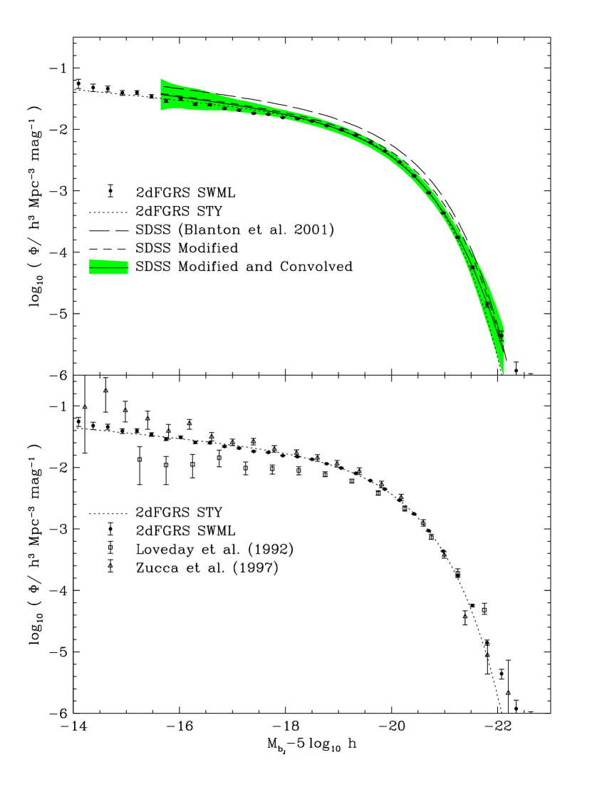
Figure 12: Comparison of the 2dFGRS ${\rm b_{J}}$-band luminosity function with estimates from the SDSS and the earlier estimates of Loveday et al. (1992) and Zucca et al. (1997).

The short dashed line in the upper panel of Fig. 12, a Schechter function with $M_{\rm b_{J}}^{\star}-5{\log_{10}h}=-19.68$, $\alpha=-1.26$ and $\Phi^{\star}=1.56\times 10^{-2}h^{3}$Mpc^-3, is the result of making three modifications to the Blanton et al. ([2001]) curve. First, we have shifted $M_{\rm b_{J}}^{\star}$ by $0.066$ magnitudes as is appropriate if one adopts the Blair & Gilmore ([1982]) colour equation ${\rm b_{J}}=B-0.28(B-V)$ rather than ${\rm b_{J}}=B-0.35(B-V)$ used by Blanton et al. ([2001]). The latter is actually ruled out by the empirical relations found by matching the 2dFGRS catalogue with either the EIS or SDSS which are instead consistent with the former. Second, we have shifted $M_{\rm b_{J}}^{\star}$ by a further $0.058$ to take account of the zeropoint offset between the SDSS and 2dFGRS photometry that we found in Section 3.1 (Fig. 3c). Finally, we have reduced $\Phi^{\star}$ by $24\%$, the reduction required for this luminosity function to reproduce the mean 2dFGRS number counts at ${\rm b_{J}}=19.2$ assuming our standard k+e-correction model. We note that Yasuda et al. ([2001]) also found a value of $\Phi^{\star}$ significantly lower than Blanton et al. when they normalized the SDSS ${\rm g}$-band luminosity function using the SDSS galaxy counts. The Yasuda et al. estimate is still higher than our value for two reasons. First the Yasuda et al. counts are 8.4% high as they include extended sources that do not satisfy all the galaxy selection criteria used in the main SDSS galaxy sample. Second although the SDSS galaxy counts agree with 2dFGRS in the area of overlap, this smaller area ($173\,$deg²) has a 5% higher density of galaxies than the full area ($1834\,$deg²) covered by the 2dFGRS survey (see Section 7). This modified SDSS Schechter function is in near perfect agreement with the Schechter function estimated from the 2dFGRS.

At the brightest magnitudes, the 2dFGRS SWML estimate is above both the 2dFGRS STY estimate and the modified SDSS Schechter function estimate. As we have seen, the main reason for this is that magnitude measurement errors in the 2dFGRS have a significant effect on the bright end of the luminosity function, but little effect around $M^{\star}$ and fainter. The solid curve surrounded by the shaded region shows the result of convolving the modified SDSS estimate with the model of the 2dFGRS magnitude errors shown in Fig. 3. The shaded region indicates the statistical error on the SDSS estimate and was read from figure 6 of Blanton et al. ([2001]). Comparing this with the 2dFGRS SWML estimate we see that the two are perfectly consistent, with the larger 2dFGRS sample having significantly smaller statistical errors.

We have seen that after taking into account the zeropoint photometric offset and the error in the colour equation, the only significant difference between the LF estimates of Blanton et al. ([2001]) and the 2dFGRS is a difference in $\Phi^{\star}$. This difference arises not because the density of galaxies is higher in SDSS than 2dFGRS (the counts agree to 5%), but because of the different methods used to constrain $\Phi^{\star}$. Blanton et al. used the method of Davis & Huchra ([1982]) which weights galaxies as a function of redshift in order to obtain a minimum variance estimate of the galaxy density. This method gives more weight to galaxies at high redshift than the method based on normalizing to the counts. It results in a smaller statistical error in the normalization, but at the same time renders the result more dependent on the accuracy of the evolutionary correction. We have seen in Section 8.1 that, even with the low redshift constraint provided by the galaxy counts, the uncertainty in $\Phi^{\star}$ due to the uncertainty in the k+e correction is significant. With the Davis & Huchra weighting this uncertainty becomes dominant. The analysis by Blanton et al. did not take account of evolution – only k-corrections were applied – and this appears to have given rise to an artificially high estimate of $\Phi^{\star}$ in the ${\rm g}$-band. We conclude that, when normalized in the same way, there is excellent agreement between the SDSS and 2dFGRS luminosity functions and that the dominant remaining uncertainty in the present day ${\rm b_{J}}$-band LF is due to residual uncertainties in evolutionary corrections.

Figure 13: Redshift distributions in the 2dFGRS and mock catalogues. The histograms show the observed redshift distribution in the NGP and SGP regions of the 2dFGRS. The left-hand panels are to the full depth of the survey while the right-hand panels include only galaxies brighter than ${\rm b_{J}}=18.5$. The smooth solid curves show the predicted redshift distributions based on our Schechter function estimate of the galaxy luminosity function, including the magnitude measurement errors, the variation in the survey magnitude limit and the dependence of completeness on apparent magnitude. The dotted lines indicate the rms variation in the redshift histograms within our ensemble of 22 mock galaxy catalogues.

The lower panel of Fig. 12 compares the 2dFGRS result with the earlier estimates of Loveday et al. ([1992]) and Zucca et al. ([1997]). We see that the Zucca et al. estimate agrees well with 2dFGRS although it has statistical errors that are much larger. The main difference with the luminosity function of Loveday et al. ([1992]) is its lower $\Phi^{\star}$. Both the 2dFGRS and Loveday et al. estimates are based on catalogues extracted from the APM survey. However, the Loveday et al. sample is much brighter and almost disjoint from the sample analyzed in this paper. As we have seen, the bright galaxy number counts in the SGP drop below model predictions extrapolated from fainter magnitudes (Maddox et al. [1990a] and Section 7) and it is therefore not surprising that Loveday found a lower value of $\Phi^{\star}$. Similarly, the flatter faint end slope that they find might be attributed, at least in part, to small volume effects. This explanation has been argued by Zucca et al. , who find they are able to accurately reproduce the Loveday et al. result if they analyze only the subset of their galaxy sample brighter than the ${\rm b_{J}}<17.15$ limit of Loveday et al. ([1992]).

10 The 2dFGRS Selection Function

The luminosity function we have derived, combined with the maps defining the survey magnitude limit (see figure 13 [2001]), redshift completeness (see Fig. 1) and $\mu$-parameter (see Fig. 15) specify the complete selection function of the 2dFGRS. It is interesting to compare the redshift distribution implied by this selection function with the measured distribution. Note that the luminosity function estimators we employed are insensitive to clustering and so the information contained in the redshift distribution of the galaxies has not been used in determining our model of the selection function.

Figure 14: As Fig. 13, but for two selected mock catalogues rather than the genuine 2dFGRS.

In Fig. 13 we compare the smooth redshift distribution predicted by our model of the 2dFGRS selection function with the observed distribution. The left-hand panels show the redshift distributions for the full 2dFGRS survey split into the SGP and NGP regions. The right-hand panels show the distributions only for galaxies brighter than ${\rm b_{J}}=18.5$. The dotted lines indicate the rms variation in the redshift histograms found in our 22 mock 2dFGRS catalogues. Gravitational clustering produces a pattern of galaxy clustering that is non-gaussian, composed of voids, walls, filaments and clusters (e.g. see figures 8 to 15 of Cole et al. [1998] for mock 2dFGRS and SDSS cone plots). As a result, the rms variation in the $N(z)$ distribution does not give an adequate description of the variation seen in the mock catalogues. For this reason we show in Fig. 14 two examples of the redshift distributions found in our ensemble of mock catalogues. From these we see that the few large spikes present in the $N(z)$ of the 2dFGRS data are common features in the mock catalogue redshift distributions.

The redshift distribution in the 2dFGRS NGP has a large spike close to the peak of the selection function and otherwise lies within 1-$\sigma$ of our smooth selection function. Thus, the density field in the NGP strip looks in no way unusual when compared to the expectation in the standard $\Lambda$CDM ($\Omega_{0}=0.3$, $\Lambda_{0}=0.7$) universe. In contrast, the density field in the SGP appears more extreme. Focusing first on the redshift distribution below $z<0.2$, we see that the observed galaxy density is nearly always below the mean density predicted by the selection function. This behaviour is consistent with the steep APM galaxy number counts, first noted by Maddox et al. ([1990a]), and discussed in Section 7 above. A lower than average galaxy density over such a large range of redshift is certainly not a common occurrence. However, as illustrated by the example of the mock SGP plotted in Fig. 14, which in many respects is quite similar to the observed 2dFGRS SGP, comparable variations do occur in the mock $\Lambda$CDM catalogues. The two examples plotted in Fig. 14 were not chosen at random, but as we only have 22 mocks to choose from, they do not represent extreme possibilities.

The 2dFGRS SGP strip also appears to show an overdensity, relative to the mean implied by the selection function, in the redshift range $0.2<z<0.25$. As the volume contributing to this redshift interval is very large, a variation as extreme as this is very unlikely. It therefore seems implausible that this perturbation in $N(z)$ is due solely to large-scale structure. There are some structures at this redshift that contribute to the excess, but even if they are excised the $N(z)$ remains higher than the model. At $z>0.2$ the only galaxies which make it into the 2dFGRS are one to two magnitudes brighter than $M^{\star}$, where the galaxy luminosity function is very steep. Thus, a small shift in magnitude can result in a large change in the number of galaxies brighter than the survey magnitude limit. We cannot reject the possibility of a small offset between the absolute calibration of the NGP and SGP; indeed, Section 3 has indicated an offset of $0.058$ magnitudes – assuming both EIS and SDSS photometry to be perfect. This is in the sense required to understand Fig. 13, i.e. the SGP is effectively deeper than the NGP. Any true offset cannot be much larger than this, otherwise it would spoil the good agreement of the STY LFs in Fig 11. Nevertheless, an NGP–SGP offset of between 0.05 and 0.1 magnitudes would yield a better match to $N(z)$ at $z>0.2$, and this possibility must be borne in mind, pending further tests against CCD data. Another possibility that needs further investigation is that the random magnitude measurement errors become larger for faint objects at high $z$. A trend of this sort is not evident in the comparison we have made between 2dFGRS and SDSS EDR magnitudes in Fig 3, but this comparison pertains to the NGP only. For now one should be careful, as we have been in previous papers, to ensure that large-scale clustering results are not strongly influenced by this feature. For instance, the estimate of the large scale galaxy power spectrum in Percival et al. ([2001]) used separate selection functions, which empirically matched the high-$z$ $N(z)$ in both NGP and SGP.

11 Discussion and Conclusions

We have described the calibration of the 2dFGRS photometry and used the CCD data of the SDSS EDR ([2002]) to assess the accuracy and completeness of the 2dFGRS photometric catalogue, which is based on APM scans of the UKST photographic plates ([1990c]). We find that the measurement errors in the APM magnitudes are in agreement with previous estimates, having a 1-$\sigma$ spread (robustly estimated) of $0.164$ magnitudes. We find a small zeropoint offset between the SDSS EDR and the 2dFGRS photometry of $|\Delta|=0.058$ and no evidence for any scale error in the magnitude calibration in the range $17<{\rm b_{J}}<19.5$. As more calibrating data become available, the accuracy of both the 2dFGRS and SDSS photometric zeropoints should be improved. We find that compared to the SDSS photometric catalogue, the 2dFGRS parent catalogue is $91\pm 2$% complete. This agrees with the original estimates based on the accuracy of star-galaxy classification in the APM catalogue ([1990b]). The reasons behind the $9\pm 2$% of galaxies that are missed are investigated in more detail in Cross et al. ([2002b]), who compare the 2dFGRS parent catalogue with the MGC, a deep, wide area B-band CCD imaging survey ([2002]). They find that mis-classification (e.g. galaxies incorrectly classified as merged images or stars) is the largest cause of incompleteness, but also a small population of low surface brightness galaxies is missed.

Making simple statistical corrections for incompleteness, magnitude measurement errors and uncertainties in modelling evolution and k-corrections, we find that the true $z=0$ galaxy luminosity function is accurately described by a Schechter function with parameters: $M^{\star}_{\rm b_{J}}-5{\log_{10}h}=-19.66\pm 0.07$, $\alpha=-1.21\pm 0.03$ and $\Phi^{\star}$$=(1.61\pm 0.08)\times 10^{-2}h^{3}$Mpc^-3 (assuming an $\Omega_{0}=0.3$, $\Lambda_{0}=0.7$ cosmology). With over 110 500 redshifts, the statistical errors in our estimate are negligible compared to the systematic errors (i.e.  uncertainties that cause an overall shift of the luminosity function) from fluctuations produced by large-scale structure and by the uncertainty in the evolutionary corrections. Our quoted errors include estimates of these uncertainties, the former derived from extensive, realistic mock catalogues.

Taking account of the photometric zeropoint difference, random magnitude measurement errors, and using an accurate colour equation, we find very good agreement between the form of the ${\rm b_{J}}$-band LF inferred from the SDSS data and the 2dFGRS estimate. Also, in the area of overlap, the 2dFGRS and SDSS galaxy counts agree at ${\rm b_{J}}=19.2$. This is the magnitude at which we use the counts to normalize our luminosity function. Thus, when normalized in the same way, 2dFGRS and SDSS ${\rm b_{J}}$-band LF estimates agree with great accuracy. Blanton et al. ([2001]) reached a different conclusion principally because they used an inaccurate colour equation to convert from SDSS wavebands to ${\rm b_{J}}$ and did not take account of galaxy evolution.

The integrated $z=0$ ${\rm b_{J}}$-band luminosity density implied by the 2dFGRS LF is $(1.82\pm 0.17)\times 10^{8}h$ L_⊙Mpc^-3. This is in good agreement with earlier estimates from the 2dFGRS presented in Folkes et al. ([1999]) and Madgwick et al. ([2002]) although neither of these estimates took account of the small effect of modelling evolution and the Folkes et al. estimate assumed an $\Omega_{0}=1$ cosmology. The dependence of the estimated luminosity density on corrections made for low surface brightness galaxies is studied in Cross et al. ([2002b]), which supercedes Cross et al. ([2001a]). The earlier paper modelled the 2dFGRS magnitudes as gaussian-corrected isophotal magnitudes, in the same way as Blanton et al. ([2001]). Ignoring the manner in which the 2dFGRS magnitudes are calibrated using deeper CCD magnitudes led to an overestimate of the amount of light lost. Cross et al. ([2002b]) show that the luminosity function estimated here agrees well with an estimate from the deeper MGC catalogue and that dependencies on surface brightness only significantly affect the luminosity function fainter than $M_{\rm b_{J}}-5{\log_{10}h}=-16.5$. Consequently the systematic effect on the estimated luminosity density is only 5 to 10%.

Wright ([2001]) has highlighted that the luminosity density measured in the optical bands by the SDSS ([2001]), combined with a simple model for the expected mean spectrum, predicts a luminosity density in the ${\rm K}_{\rm S}$-band a factor of $2.3$ greater than the value measured in the joint analysis of 2MASS ([2000]) and 2dFGRS presented in Cole et al. ([2001]). Note that Kochanek et al. ([2001]) found a very similar ${\rm K}_{\rm S}$-band luminosity density to that found by Cole et al. ([2001]), but their estimate used 2MASS isophotal magnitudes for which the correction to total magnitudes is more uncertain. Even if the SDSS luminosity densities were to be revised downwards to agree with the 2dFGRS in the ${\rm b_{J}}$-band, the discrepancy in the ${\rm K}_{\rm S}$-band would only be reduced to a factor of $1.6$. Furthermore, the correction for longer wavelength bands is likely to be smaller than that we have inferred for the ${\rm g}$-band. Thus, a puzzling factor of approximately $1.8$ to $2$ remains between the ${\rm K}_{\rm S}$-band luminosity density measured from 2MASS and that inferred by extrapolation from the optical bands.

Wright ([2001]) speculated that the 2MASS fluxes could be grossly underestimated. This possibility is ruled out by the comparison of 2MASS magnitudes with those from deeper, high resolution ${\rm K}_{\rm S}$-band images. Cole et al. ([2001]) compared 2MASS magnitudes with Kron magnitudes measured for the same objects by Loveday ([2000]) and found that only a $0.06$ magnitude correction was needed to bring them into agreement. A somewhat larger larger offset, but still only 20%, has been argued for by Andreon ([2002]). Furthermore, combining the 2MASS and SDSS EDR magnitudes for matched objects, we find optical to near infrared colours which, on average, agree well with the mean galaxy spectrum adopted by Wright. A second speculation made by Wright was that perhaps the 2MASS extended source catalogue is incomplete and misses a significant fraction of the galaxies that SDSS detects. This is also appears unlikely. The assessment of the completeness of 2dFGRS compared to 2MASS presented in Cole et al. ([2001]), together with the assessment of the 2dFGRS completeness with respect to the SDSS presented here, shows that the 2MASS and SDSS source densities agree to about 2%.

The most likely cause of the discrepancy between the ${\rm K}_{\rm S}$-band and extrapolated optical luminosity densities is large-scale structure. Since the 2MASS survey has a much brighter limiting magnitude than either the 2dFGRS or SDSS, their luminosity functions are not normalized within the same volume. Cole et al. ([2001]) normalized their ${\rm K}_{\rm S}$-band LF using an estimate of the counts from a small, $184\,$deg² area (Jarrett et al. in preparation) and an indirect estimate from the approximately $619\,$deg² of overlap between 2MASS and 2dFGRS. The second estimate is perhaps not highly accurate, because it requires an estimate of the effective area of sky in the intersection of the 2dFGRS and 2MASS. This is not trivial to obtain because a map of the 2MASS sky coverage is not yet available. Cole et al. ([2001]) estimated that large-scale structure would cause a 15% variation in the number counts within a $619\,$deg² area. Our mock catalogues, modified to mimic the selection criteria of the 2MASS, show that the rms variation in the counts over a $184\,$deg² area is, significantly larger, 19%. Thus, it will be very interesting to derive the ${\rm K}_{\rm S}$-band counts over a larger area, which should soon become possible with a more complete 2MASS catalogue, to see whether the estimates of the J and ${\rm K}_{\rm S}$-band luminosity densities and the inferred stellar density need to be revised.

We have described maps that define the redshift completeness of the current 2dFGRS catalogue and the weak dependence of the degree of completeness on apparent magnitude. These, together with the luminosity function and a map of the survey magnitude limit, provide a complete description of the 2dFGRS selection function. We have created mock galaxy catalogues from cosmological N-body simulations using this description of the selection function. Comparison of these with the observed data indicates that, in general, the data are well described by our selection function and exhibit fluctuations that are typical of those expected in the standard $\Lambda$CDM cosmology.

Appendix A Redshift Incompleteness in the 2dFGRS

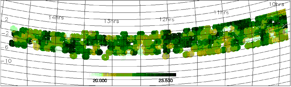
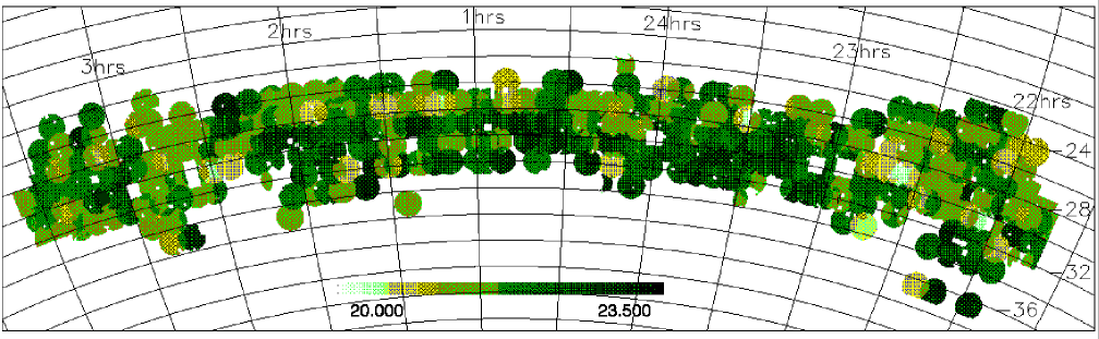
Figure 15: Map showing the variation of the parameter $\mu$ with position on the sky. The dependence of the redshift completeness on apparent magnitude is accurately described by the fitting function $c_{z}({\rm b_{J}},\mu)=0.99\left(1-\exp[{\rm b_{J}}-\mu]\right)$.

When complete, the fraction of redshifts measured should be uniformly high across the full area of the 2dFGRS. However, at this intermediate stage, when only a subset of the target 2dF fields have been observed, the fraction of redshifts measured varies considerably with position. As detailed in Section 8 of Colless et al. ([2001]), this variation is best quantified by dividing the survey into sectors (labelled by an angular position ${\mn@boldsymbol{\theta}}$) defined by the overlaps of the target 2dF fields. Within each of these sectors one can calculate the fraction $R({\mn@boldsymbol{\theta}})$ of the parent catalogue galaxies whose redshifts have been measured. It is this completeness map, pixellated for convenience, that is shown in Fig. 1.

In contrast to most previous redshift surveys, the 2dFGRS is so large that residual small systematic errors can begin to dominate over statistical errors. For this reason, we have developed a quantitative description of the dependence of the completeness on apparent magnitude. Note that 76% of the observed fields have an overall completeness of greater than 90% (this should increase with time as some of the lower completeness fields are re-observed) and so generally incompleteness and its dependence on apparent magnitude are small. In Section 8.3 of Colless et al. ([2001]), we showed that for each observed field the dependence of the redshift completeness on apparent magnitude could be described by a one parameter function (see figure 16 of [2001])

$$c_{z}({\rm b_{J}},\mu_{i})=0.99\,\left(1-\exp[{\rm b_{J}}-\mu_{i}]\right).$$ (8)

Here ${\rm b_{J}}$ is the apparent magnitude and $\mu_{i}$ is the value of the parameter for field $i$. In each sector, the targeted galaxies are split between several fields and so one must define an appropriately averaged value, $\mu({\mn@boldsymbol{\theta}})$, for each sector. This can be derived by writing the magnitude-dependent redshift incompleteness of a sector $c_{z}({\rm b_{J}},\mu({\mn@boldsymbol{\theta}}))$ as a weighted sum of the completeness of its $N_{\rm F}({\mn@boldsymbol{\theta}})$ component fields,

$$c_{z}({\rm b_{J}},\mu[{\mn@boldsymbol{\theta}}])=\sum_{i=1}^{N_{\rm F}({\mn@boldsymbol{\theta}})}f_{i}\,c_{z}({\rm b_{J}},\mu_{i}),$$ (9)

where $f_{i}$ is the fraction of observed galaxies in this sector that were targeted in field $i$. Hence by identification of terms

$$c_{z}({\rm b_{J}},\mu_{i})=0.99\,\left(1-\exp[{\rm b_{J}}-\mu({\mn@boldsymbol{\theta}})]\right),$$ (10)

where

$$\mu({\mn@boldsymbol{\theta}})=-\ln\left[\sum_{i=1}^{N_{\rm F}({\mn@boldsymbol{\theta}})}f_{i}\,\exp(-\mu_{i})\right].$$ (11)

With this one can define the function

$$S({\mn@boldsymbol{\theta}},{\rm b_{J}})=R({\mn@boldsymbol{\theta}})\,c_{z}({\rm b_{J}},\mu[{\mn@boldsymbol{\theta}}])/\bar{c}_{z}(\mu[{\mn@boldsymbol{\theta}}])$$ (12)

which is an estimate of the fraction of galaxies of apparent magnitude ${\rm b_{J}}$ in the sector at position ${\mn@boldsymbol{\theta}}$ that have redshift measurements. Here $\bar{c}_{z}(\mu[{\mn@boldsymbol{\theta}}])$ is $c_{z}({\rm b_{J}},\mu[{\mn@boldsymbol{\theta}}])$ averaged over the expected apparent magnitude distribution of the galaxies in the sector.

Maps of ${\rm b_{J}}^{\rm lim}({\mn@boldsymbol{\theta}})$, $R({\mn@boldsymbol{\theta}})$ and $\mu({\mn@boldsymbol{\theta}})$ together with associated software are available for the 2dFGRS data in the 100k Release (http://www.mso.anu.edu.au/2dFGRS/). Here, we employ the method described in section 8 of Colless et al. ([2001]) to generate these quantities for the more extensive dataset used in this paper. The map of $R({\mn@boldsymbol{\theta}})$ is shown in Fig. 1 and the corresponding map of $\mu({\mn@boldsymbol{\theta}})$ is shown in Fig. 15.

References

- [2002] Andreon S., 2002, A&A, 382, 495
- [1997] Arnouts S., de Lapparent V., Mathez G., Mazure A., Mellier Y., Bertin E., Kruszewski A, 1997, A&AS, 124, 163
- [2001] Arnouts S., et al. , 2001, A&A, 379, 740. (astro-ph/0103071)
- [ 1993] Baugh C. M., Efstathiou G., 1993, MNRAS, 265, 145
- [2002] Baugh C.M., Branchini E., Cole S., 2002 in preparation
- [1996] Bertin E., Arnouts S., 1996, A&A Suppl., 117, 393
- [1982] Blair M., Gilmore G., 1982, PASP, 94, 741
- [2001] Blanton M.R., et al. 2001, AJ, 121, 2358 (astro-ph/0012085)
- [1993] Bruzual A. G., Charlot S., 1993, ApJ, 405, 538
- [1993] Caretta, C.A., Maia, M.A.G., Willmer, C.N.A., 2000, AJ, 119, 524
- [2001] Charlot S., Longhetti M., 2001, MNRAS, 323 887
- [1994] Cole S., Aragon-Salamanca A., Frenk C.S., Navarro J.F., Zepf S.E., 1994, MNRAS, 271, 781
- [1998] Cole S., Hatton S., Weinberg D.H., Frenk C.S., 1998, MNRAS, 300, 945
- [2000] Cole S., Lacey C.G., Baugh C.M., Frenk C.S., 2000, MNRAS, 319, 168
- [2001] Cole S., et al. (The 2dFGRS Team) 2001, MNRAS, 326, 255
- [2001] Colless M., et al. (the 2dFGRS team) 2001, MNRAS, 328, 1039 (astro-ph/0106498)
- [2001a] Cross N.J.G., et al. (The 2dFGRS Team) 2001a, MNRAS, 324, 825
- [2002] Cross N.J.G., & Driver, S.P. 2002, MNRAS, 329, 579. (astro-ph/0110402)
- [2002b] Cross N.J.G., et al. (The 2dFGRS Team) 2002b, in preparation.
- [1982] Davis M., Huchra J., 1982, ApJ, 254, 437
- [1999] Driver S.P., 1999, ApJ, 526, L69
- [1988] Efstathiou G., Ellis R.S., Peterson B.A., 1988, MNRAS 232, 431
- [1999] Evrard A.E., 1999, in proceedings of the MPA-ESO cosmology conference 1998, “Evolution of large scale structure : from recombination to Garching” eds A. J. Banday, R. K. Sheth, and L. N. da Costa, Garching, Germany : European Southern Observatory, p.249 (astro-ph/9812377)
- [2002] Evrard A.E., et al. 2002, ApJ submitted (astro-ph/0110246)
- [1976] Felten J. E., 1976, ApJ 207, 700
- [1994] Ferguson H.C., Binggeli B., 1994, A&AR 6, 67
- [1999] Folkes S., et al. (2dFGRS Team), 1999, MNRAS, 308, 459
- [1996] Fukugita M., Ichikawa T., Gunn J.E., Doi M., Shimasaku K., Schneider D.P., 1996, AJ, 111, 1754
- [1994] Irwin M., Maddox S., Mcmahon R. 1994, Spectrum, 2, 14
- [2000] Jarrett T.H., Chester T., Cutri R., Schneider S., Skrutskie M., Huchra, J.P., 2000, AJ, 119, 2498
- [1993] Kauffmann G., White S.D.M., Guiderdoni B., 1993, MNRAS, 264, 201
- [1992] Katz N., Hernquist L., Weinberg D.H., 1992, ApJ, 399, 109
- [2001] Kochanek C.S., Pahre M.A., Falco E.E., Huchra J.P., Mader J., Jarrett T.H., Chester T., Cutri R., Schneider S.E., 2001, ApJ, 560, 566
- [2002] Lemon D.J., Liske J., Driver S.P., Cross N.J.G., Couch W.J., 2002, in preparation
- [1996] Lewis G., Irwin M., 1996, Spectrum, 12, 22
- [1996] Lin H., Kirshner R.P., Shectman S.A., Landy S.D., Oemler A., Tucker D.L., Schechter P. L., 1996, ApJ, 471, 617
- [1993] Liu M.C., Charlot S., Graham J.R., 2000, ApJ, 543, 644
- [1992] Loveday J., Peterson B. A., Efstathiou G., Maddox S.J., 1992, ApJ, 390,338
- [1996] Loveday J., Peterson B. A., Maddox S.J., Efstathiou G., 1996, ApJS, 107, 201
- [2000] Loveday J., 2000, MNRAS, 312, 517
- [1990a] Maddox S.J., Sutherland W.J., Efstathiou G., Loveday J., Peterson B.A., 1990a, MNRAS, 247, 1
- [1990b] Maddox S.J., Efstathiou G., Sutherland W.J., Loveday J., 1990b, MNRAS 243, 692 (APMI)
- [1990c] Maddox S.J., Efstathiou G., Sutherland W.J., Loveday J., 1990c, MNRAS 246, 433 (APMII)
- [1996] Maddox S.J., Efstathiou G., Sutherland W.J., Loveday J., 1996, MNRAS 283, 1227 (APMIII)
- [2002] Maddox S.J., et al. , (The 2dFGRS Team) 2002, in preparation.
- [2002] Madgwick D.S., et al. , (The 2dFGRS Team), 2002, MNRAS in press. (astro-ph/0107197)
- [1994] Marzke R.O., Huchra J.P., Geller M.J., 1994, ApJ., 428, 43
- [1995] Metcalfe N., Fong R., Shanks T., 1995, MNRAS, 274, 769
- [2001a] Norberg P., et al. (The 2dFGRS Team) 2001a, MNRAS, 328, 64
- [2001b] Norberg P., 2001b, Durham University Ph.D. Thesis.
- [2002] Norberg P., et al. (The 2dFGRS Team) 2002, MNRAS, 332, 827
- [2001] Pearce F.R., Jenkins A., Frenk C.S., White S.D.M., Thomas P.A., Couchman H.M.P., Peacock, J.A., Efstathiou, G., 2001, MNRAS, 326, 649
- [2001] Percival W.J., et al. (The 2dFGRS Team) 2001, MNRAS, 327, 1297 (astro-ph/0105252)
- [2001] Pimbblet K.A., Smail I., Edge A.C., Couch W.J., O’Hely E., Zabludoff A.I., 2001, MNRAS, 327, 588
- [1999] Prandoni I., et al. 1999, A&A 345, 448
- [1998] Ratcliffe A., Shanks T., Parker Q.A., Fong R., 1998, MNRAS, 294, 147
- [1994] Raychaudhury S., Lynden-Bell D., Scharf C., Hudson M.J., 1994, BAAS, 184, No. 3806
- [1979] Sandage A., Tammann G.A., Yahil A., 1979, ApJ 232, 352
- [1976] Schechter P., 1976, ApJ, 203, 297
- [1998] Schlegel D.J., Finkbeiner D.P., Davis M., 1998, ApJ, 500, 525
- [2002] Shao Z., Maddox S.J., Jones B., Coles P., 2002, MNRAS, submitted.
- [1999] Somerville R., Primack J.R., 1999, MNRAS, 310, 1087
- [2002] Stoughton C., et al. , (The SDSS Collaboration), 2002 AJ, 123, 485
- [2002] Strauss M.A., et al. , (The SDSS Collaboration), 2002 in preparation
- [1991] White S.D.M., Frenk C.S., 1991, ApJ, 379, 52
- [2001] Wright E.L., 2001, ApJ, 556, 17
- [2001] Yasuda N., et al. 2001, (The SDSS Collaboration) AJ, 122, 1104 (astro-ph/0105545)
- [1997] Zucca E., et al. 1997, A&A, 326, 477