Closed Universes from Cosmological Instantons

Abstract

Current observational data is consistent with the universe being slightly closed. We investigate families of singular and non-singular closed instantons that could describe the beginning of a closed inflationary universe. We calculate the scalar and tensor perturbations that would be generated from singular instantons and compute the corresponding CMB power spectrum in a universe with cosmological parameters like our own. We investigate spatially homogeneous modes of the instantons, finding unstable modes which render the instantons sub-dominant contributions in the path integral. We show that a suitable condition may be imposed on singular closed instantons, constraining their instabilities. With this constraint these instantons can provide a suitable model of the early universe, and predict CMB power spectra in close agreement with the predictions of slow-roll inflation.

I Introduction

Recent measurements of the Cosmic Microwave Background (CMB) temperature anisotropy de Bernardis et al. (2001); Stompor et al. (2001) have been able to tightly constrain the curvature of the universe. The results indicate that the universe is close to being spatially flat, with current limits of $0.94<\Omega_{\mathrm{tot}}<1.06$ at one sigma. However closed models still take up a significant part of the possible parameter space, and unless the universe is significantly open we shall probably never be able to rule out closed models. In this paper we discuss an approach to quantum cosmology which yields closed inflationary universes consistent with the current observations.

Over the past three years there has been a development of methods treating open universes Garriga et al. (1998); Hawking and Turok (1998); Gratton and Turok (1999); Hertog and Turok (2000); Gratton et al. (2000); Gratton and Turok (2001) in the context of Euclidean quantum cosmology Hartle and Hawking (1983). In this paper we adapt these methods to closed universes, and use them to calculate the perturbation power spectrum for such models. The reader is referred to the above papers for general details; here we mainly emphasize the new considerations arising from the closed geometry. In many ways the closed calculations are easier, with the spatial hypersurfaces being compact and the analytic continuation being simpler. A major difference is that a different variable must be used to represent the scalar fluctuations about the instanton in the closed case, due to the different ranges of the background variables.

The structure of this paper is as follows. We firstly describe non-singular and singular closed instantons and their analytic continuations to possible universes. We then introduce variables suitable for the description of scalar fluctuations across the entire instantons and show that in both cases negative modes exist which render these instantons unstable. For the non-singular case we show that at least two negative modes exist, excluding these from even speculative tunneling applications Coleman (1988). In the singular case we are able to motivate a constraint at the singularities Kirklin et al. (2001), which projects out these negative modes. We then proceed to calculate the predicted scalar and tensor perturbations about such constrained singular closed instantons. We calculate the two-point correlation functions in the Euclidean region and analytically continue these expressions into the Lorentzian region. We compute the power spectra at the end of inflation and use these as initial conditions for the radiation dominated era in to order to compute the predicted CMB power spectra for a given cosmological model. The suitability of these models as descriptions of the early history of our universe is then commented upon.

II Instantons for Closed Universes

Consider a closed universe with line element

$$ds^{2}=-dt^{2}+a^{2}(t)d\Omega_{3}^{2}$$ (1)

and scalar field $\phi$ with potential $V(\phi)$. The Friedmann Equation reads

$$\left(\frac{\dot{a}}{a}\right)^{2}=\frac{\kappa}{3}\left(\frac{1}{2}{\dot{\phi}}^{2}+V(\phi)\right)-\frac{{\cal K}}{a^{2}}$$ (2)

where ${\cal K}$ is the spatial curvature constant, with ${\cal K}>0$ corresponding to a closed universe. One sees that it is possible for both $a$ and $\phi$ to be stationary at the same time, $t=0$ say, if at this moment $a$ and $\phi$ are such that $\kappa a^{2}V/3={\cal K}$. Around $t=0$, $a$ and $\phi$ will then have power series expansions even in $t$. Hence one may consider the analytic continuation $\sigma=it$, under which both $a$ and $\phi$ remain real. The line element then takes the Euclidean form

$$ds^{2}=d\sigma^{2}+b^{2}(\sigma)d\Omega_{3}^{2}$$ (3)

with $b(\sigma)$ the radius of the three-sphere, related to $a$ by $b(\sigma)=a(-i\sigma)$. The Einstein and scalar field equations take the form

$$\phi_{,\sigma\sigma}+3{\frac{b_{,\sigma}}{b}}\phi_{,\sigma}=V_{,\phi},\qquad b_{,\sigma\sigma}=-{\frac{\kappa}{3}}b\left(\phi_{,\sigma}^{2}+V\right)$$ (4)

where $\kappa\equiv 8\pi G$, $\phi_{,\sigma}\equiv\partial_{\sigma}\phi$ and $V_{,\phi}\equiv\frac{dV}{d\phi}$. There are solutions to these equations with various geometries. For the open case of Ref. Gratton and Turok (1999) the background metric and scalar field behaved appropriately at a pole. Here we are interested in solutions symmetric about an equator (where $b_{,\sigma}=0$) that have continuations into a real closed universe.

One can introduce conformal coordinates in both the Euclidean and Lorentzian regions, defined by integrating $dX=-bd\sigma$ and $d\tau=adt$ from the matching surface. In this closed case, since the scale factor is finite at the matching point, the conformal coordinates $X$ and $\tau$ behave just like $\sigma$ and $t$ and can be continued into each other similarly. This is another significant simplification when compared to the open case.

By virtue of the boundary conditions required by the continuation we see that $b$ and $\phi$ must be symmetrical about the equator of the instanton. For potentials $V$ greater than or equal to zero, evolving the equation for $b$ from the equator enables one to see that $b$ must twice reach zero a finite distance in $\sigma$ away, at $\pm\sigma_{m}$ say. These are poles of the instanton. Because of the the symmetry about the equator they must be of the same form and can either be regular or singular, as discussed in detail in Refs. Hawking and Turok (1998); Gratton and Turok (1999). Singular instantons exist for almost any scalar field potential, whereas the regular instantons can only exist for potentials which have a local maximum and are sufficiently negatively curved in the region of the peak (from the work of Jensen and Steinhardt (1984) we require that $-3V_{,\phi\phi}/\kappa V>10$). See the illustration in Fig. 1.

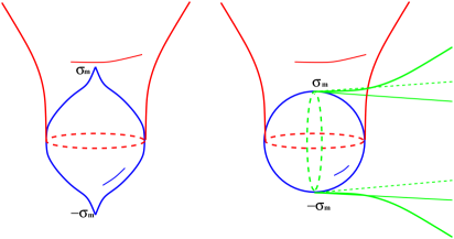
Figure 1: This figure illustrates the continuation from singular (left) and non-singular (right) instantons into Lorentzian universes. Analytic continuation at the equator yields a closed universe. In the non-singular instanton continuation at the poles gives open universes.

To reiterate, the key difference between open and closed instantons is that the former have their boundary conditions imposed by behavior at a pole whereas the latter have their boundary conditions imposed by behavior at the equator. One might ask if these conditions ever overlap. Indeed they do, as it is possible to continue any regular closed instanton not from its equator into a closed universe but from one of its poles into an open universe. From the open point of view, these correspond to the “multibounce” instantons mentioned in Sec. 3 of Gratton and Turok (1999). From the negative mode argument presented there, one immediately suspects that these solutions will have more than one negative mode and hence not be relevant for cosmological applications. Indeed, we will prove below that a large class of these non-singular models have at least two negative modes.

We now turn to investigate the scalar fluctuations about these instantons.

III The Second Order Action

Our starting point is the second order action for scalar perturbations in the Lorentzian universe, as discussed in Sec. 4 of Gratton and Turok (1999), to which we refer the reader for definitions. The result we use agrees with that given in Mukhanov et al. (1992) up to a surface term, and is reproduced here,

$$S_{2} = \frac{1}{2\kappa}\int d\tau d^{3}xa^{2}\sqrt{\gamma}\bigg{\{}-6\psi^{\prime}{}^{2}-12{\cal H}A\psi^{\prime}+2\Delta\psi\left(2A-\psi\right)-2\left({\cal H}^{\prime}+2{\cal H}^{2}\right)A^{2}$$ (5)

$$+\kappa\left({\delta\phi}^{\prime}{}^{2}+{\delta\phi}\Delta{\delta\phi}-a^{2}V_{,\phi\phi}{\delta\phi}^{2}\right)+2\kappa\left(3{\phi^{\prime}}\psi^{\prime}{\delta\phi}-{\phi^{\prime}}{\delta\phi}^{\prime}A-a^{2}V_{,\phi}A{\delta\phi}\right)$$

$$+{\cal K}\left(-6\psi^{2}+2A^{2}+12\psi A+2\left(B-E^{\prime}\right)\Delta\left(B-E^{\prime}\right)\right)$$

$$+4\Delta\left(B-E^{\prime}\right)(\frac{\kappa}{2}{\phi^{\prime}}{\delta\phi}-\psi^{\prime}-{\cal H}A)\bigg{\}}.$$

This is well defined for all values of ${\phi^{\prime}}$ and the three-space Laplacian $\Delta$. In a closed universe ${\cal K}>0$ and the eigenvalues of $\Delta$ are given by $-{\cal K}(n^{2}-1)$, where $n$ is a positive integer.

For the spatially inhomogeneous modes $(n\geq 2)$ we introduce the momenta canonically conjugate to $\psi$, $E$, and ${\delta\phi}$ and rewrite the action in first-order form, as in Eq. (20) of Gratton and Turok (1999). Then we integrate over $B$, leaving us with a delta functional for $\Pi_{E}$. Integrating over this effectively sets $\Pi_{E}$ to zero. For the homogeneous $(n=1)$ mode $B$ and $E$ disappear from the action, so we can only introduce momenta canonically conjugate to $\psi$ and ${\delta\phi}$. However the action can still be rewritten in first-order form, and has the same form as in the inhomogeneous case. So we now have the following expression for all modes in terms of $\psi$, $\Pi_{\psi}$, ${\delta\phi}$, $\Pi_{{\delta\phi}}$, and $A$:

$$S_{2} = \int d\tau d^{3}x\Bigg{\{}\Pi_{\psi}\psi^{\prime}+\Pi_{{\delta\phi}}{\delta\phi}^{\prime}+\frac{\kappa{\cal K}}{4a^{2}\sqrt{\gamma}\left(\Delta+3{\cal K}\right)}\Pi_{\psi}^{2}-\frac{1}{2a^{2}\sqrt{\gamma}}\Pi_{{\delta\phi}}^{2}-\frac{\kappa}{2}{\phi^{\prime}}\Pi_{\psi}{\delta\phi}$$ (6)

$$~{}~{}~{}-\frac{a^{2}\sqrt{\gamma}}{\kappa}\left(\left(\Delta+3{\cal K}\right)\psi^{2}-\frac{\kappa}{2}\left(\Delta+3{\cal K}-{\cal H}^{2}-{\cal H}^{\prime}+\frac{\phi^{\prime\prime\prime}}{{\phi^{\prime}}}\right){\delta\phi}^{2}\right)$$

$$~{}~{}~{}-A\left(-{\cal H}\Pi_{\psi}+\phi^{\prime}\Pi_{{\delta\phi}}+\frac{2a^{2}\sqrt{\gamma}}{\kappa}\left(-\left(\Delta+3{\cal K}\right)\psi+\frac{\kappa}{2}\left({\cal H}{\phi^{\prime}}-\phi^{\prime\prime}\right){\delta\phi}\right)\right)\Bigg{\}}.$$

The $n=2$ mode corresponds to a gauge degree of freedom and is ignored as discussed in Sec. 4 of Gratton and Turok (2001). We now have some choice in deciding which linear combination of variables to use in order to describe the single scalar degree of freedom of the system. As we shall see, different choices are particularly suited to different background solutions.

IV Non-singular Closed Instantons

From our experience Gratton and Turok (2001) with Hawking-Moss Hawking and Moss (1982) and Coleman-De Luccia Coleman and DeLuccia (1980) instantons one expects a variable related to ${\delta\phi}$ to be a good variable to use in treating closed instantons. We remind the reader that, as discussed in detail in Gratton and Turok (2001), a good variable is one whose Euclidean action is bounded below for all normalized fluctuations of that variable about the instanton in question. This corresponds to having a positive kinetic term in the Euclidean action for all values of $\Delta$.

We discussed closed instantons in Sec. II. The simplest instanton is that of Hawking and Moss, which has the scalar field constant and at a local maximum of the potential. It is a round $S^{4}$ and has $O(5)$ invariance. It can be analytically continued to either the closed or the open slicing of De Sitter space. The closed instantons discussed in Sec. II may, as discussed above, also be continued to open or closed inflationary universes.

Under an open continuation, we have Gratton and Turok (1999)

$$\sigma\leftrightarrow it,~{}~{}~{}X\leftrightarrow-\tau-i\pi/2,~{}~{}~{}b^{2}\leftrightarrow-a^{2},~{}~{}~{}\Delta\leftrightarrow-\Delta,~{}~{}~{}{\cal K}\leftrightarrow{\cal K},$$ (7)

whereas under a closed continuation,

$$\sigma\leftrightarrow it,~{}~{}~{}X\leftrightarrow i\tau,~{}~{}~{}b^{2}\leftrightarrow a^{2},~{}~{}~{}\Delta\leftrightarrow\Delta,~{}~{}~{}{\cal K}\leftrightarrow{\cal K},$$ (8)

as discussed above. The differing analytic continuations ensure that if one starts in the Lorentzian region in either an open or a closed slicing, one gets an identical expression when continued back to the Euclidean region. For example, the combination $\Delta+3{\cal K}$ occurs in both Lorentzian regions. This continues to $-\Delta+3{\cal K}$ in the Euclidean region from an open universe, or to $\Delta+3{\cal K}$ from a closed universe. However, ${\cal K}$ is negative in an open universe, so these two expressions really differ only by a sign. In fact, the sign is also mopped up by another minus sign originating from $a^{2}$ so that both continuations produce an identical Euclidean action, as long as we interpret ${\cal K}$ in the Euclidean region to really be $|{\cal K}|$ of the Lorentzian region. Since this paper only deals with closed universes, for which ${\cal K}$ is positive, we can ignore this subtlety.

Sec. 4 of Gratton and Turok (2001) introduced a variable which made the negative mode structure transparent. Here we attempt to adapt the argument to the case of a closed instanton. We introduce the gauge invariant perturbation variable $\delta\phi_{\text{gi}}$,

$$\delta\phi_{\text{gi}}={\delta\phi}-\frac{\kappa{\phi^{\prime}}\Pi_{\psi}}{2a^{2}\sqrt{\gamma}(\Delta+3{\cal K})}.$$ (9)

After integrating out the other variables from (6), analytically continuing to the Euclidean region, and introducing the rescaled variable $Q=b\delta\phi_{\text{gi}}/\phi^{\prime}$ we obtain the action

$$S_{2}={\frac{1}{2}}\int dXd^{3}x\sqrt{\gamma}\phi^{\prime}{}^{2}\left(\frac{Q^{\prime}{}^{2}}{1-\frac{\kappa\phi^{\prime}{}^{2}}{2\left(\Delta+3{\cal K}\right)}}-\left(\Delta+3{\cal K}\right)Q^{2}\right).$$ (10)

One might think that if $1-\kappa\phi^{\prime}{}^{2}/6{\cal K}>0$ across the instanton, so that the $Q^{\prime}{}^{2}$ always has a positive coefficient, $Q=\mathrm{const}$ might be a homogeneous negative mode. However, there are two subtleties in the closed case which did not occur in the parallel case for open-only instantons (for which $\phi^{\prime}$ is always positive.) Firstly, because the scale factor is finite on the matching surface and $\phi^{\prime}$ is zero there, $Q$ is not well defined in the closed case. Secondly, the natural measure in the open-only case was $\phi^{\prime}{}^{2}$, but in the closed case this vanishes on the equator and so is inadmissible. However the variable ${\tilde{Q}}\equiv b\delta\phi_{\text{gi}}$ is well defined, and we can proceed to derive the action in terms of this variable.

Starting from Eq. (6) we perform the path integral over $A$ which imposes a delta functional allowing us to express $\psi$ in terms of $\Pi_{\psi}$ and $\Pi_{\delta\phi}$. After integrating by parts to remove terms in the derivatives of the conjugate momenta we define $\Pi_{\tilde{Q}}$ as the variable conjugate to ${\tilde{Q}}$. Substituting $\Pi_{\delta\phi}$ for $\Pi_{\tilde{Q}}$ we find the action is independent of $\Pi_{\psi}$, and so its path integral can be neglected as an infinite gauge-orbit volume. Finally performing the Gaussian integral over $\Pi_{\tilde{Q}}$ we obtain the Euclidean action

$$S_{2} = {\frac{1}{2}}\int\frac{dXd^{3}x\sqrt{\gamma}}{1-\frac{\kappa\phi^{\prime}{}^{2}}{2(\Delta+3{\cal K})}}\left({\tilde{Q}}^{\prime}{}^{2}-\left[\Delta+3{\cal K}-{\frac{1}{2}}\kappa\phi^{\prime}{}^{2}-\frac{\phi^{\prime\prime\prime}}{\phi^{\prime}}-\frac{\kappa(\phi^{\prime\prime})^{2}}{\Delta+3{\cal K}-{\frac{1}{2}}\kappa\phi^{\prime}{}^{2}}\right]{\tilde{Q}}^{2}\right).$$ (11)

Note that $\phi^{\prime\prime\prime}/\phi^{\prime}$ is well behaved at the equator because $\phi$ is an even function for the closed instanton, and this action is suitable as long as $1-\kappa\phi^{\prime}{}^{2}/6{\cal K}>0$ across the entire instanton. One can confirm this numerically in any particular case of interest—most regular closed instantons leading to reasonable amounts of inflation satisfy this condition.

As expected one can confirm that ${\tilde{Q}}=\phi^{\prime}$ is a spatially homogeneous negative mode of the fluctuation operator associated with this action. However, $\phi^{\prime}$ is odd about the equator so this negative mode has a node. The eigenvector associated with the lowest eigenvalue must be nodeless and hence there must exist a symmetric mode function with a more negative eigenvalue. (This can be confirmed numerically by substituting a symmetric test function, ${\tilde{Q}}=b$ say, into (11) and checking that the action integral over the instanton is negative.) So we have proved that these instantons must have at least two negative modes, and therefore cannot have anything to do with tunneling Coleman (1988); Gratton and Turok (2001). This confirms explicitly the arguments based on spectral flow from the Hawking-Moss instanton given in Sec. 3 of Gratton and Turok (2001).

As far as we are aware, there is no way to constrain these instantons to eliminate their instabilities. Thus there is no motivation for considering them as being significant in the Euclidean quantum path integral. No tunneling role being apparent either, we do not consider these instantons further. Instead we now turn to singular instantons, where suitable constraints may be applied.

V Singular Closed Instantons

On singular instantons, as the scalar field runs away to infinity at the poles, the condition $1-\kappa\phi^{\prime}{}^{2}/6{\cal K}>0$ is certainly violated. This means that $\delta\phi_{\text{gi}}$ is not a suitable variable to use when investigating fluctuations around closed singular instantons.

A good physical choice of variable is the gauge invariant combination

$${\cal X}\equiv\psi+\frac{{\cal H}}{\phi^{\prime}}{\delta\phi},$$ (12)

the comoving curvature perturbation. In the gauge ${\delta\phi}=0$ this is just $\psi$. Notice that in the definition the factors ${\cal H}$ and $\phi^{\prime}$ are combined in such a way as to be finite at the equator of the instanton, since in this closed case both go linearly to zero there.

Using the definition we substitute ${\delta\phi}$ for ${\cal X}$ in Equation (6). The path integral over $A$ imposes a delta functional which allows us to express $\psi$ in terms of $\Pi_{\psi}$ and $\Pi_{\delta\phi}$. After integrating by parts to remove terms in the derivatives of the conjugate momenta we define $\Pi_{\cal X}$ as the variable conjugate to ${\cal X}$. Substituting $\Pi_{\delta\phi}$ for $\Pi_{\cal X}$ we find the action is independent of $\Pi_{\psi}$, and so its path integral can be neglected as an infinite gauge-orbit volume. Finally performing the Gaussian integral over $\Pi_{\cal X}$ and continuing to the Euclidean region we are left with

$$S_{2}=\frac{1}{\kappa}\int dXd^{3}x\frac{b^{2}\sqrt{\gamma}z^{2}}{1-z^{2}{\cal K}/(\Delta+3{\cal K})}\left({\cal X}^{\prime}{}^{2}-\left[\frac{2{\cal K}}{1-z^{2}{\cal K}/(\Delta+3{\cal K})}\frac{z^{\prime}}{z{\cal H}}+\Delta+4{\cal K}\right]{\cal X}^{2}\right)$$ (13)

where we have introduced $z\equiv\sqrt{\kappa/2}\phi^{\prime}/{\cal H}$ for clarity.

Let us now examine the behavior of this action across the instanton. For ${\cal X}$ to be a suitable variable we need the coefficient of the kinetic term to be positive everywhere. Remembering that the eigenvalues of $\Delta$ are $-{\cal K}(n^{2}-1)$, where $n$ is a positive integer (and ${\cal K}$ is a positive real number in this closed case), we see that this is indeed the case for spatially inhomogeneous fluctuations. In the homogeneous case ($n=1$) it will be positive if $1-z^{2}/3>0$ across the instanton. This can be checked numerically for any case of interest, but we can also make analytic arguments for wide classes of cosmological instantons. Let us first examine behavior near the equator. From the scalar field equation in proper Euclidean time, we have ${\dot{\phi}}\approx V_{,\phi_{0}}\sigma$ and from the equation for the scale factor we have $\dot{b}\approx-\kappa bV(\phi_{0})\sigma/3$. Hence $1-z^{2}/3\approx 1-3V_{,\phi_{0}}^{2}/2\kappa V(\phi_{0})^{2}$. For a monomial potential $\lambda\phi^{r}$, we can link the starting value $\phi_{0}$ of the field with the number $P$ of e-foldings by the relation Bucher et al. (1995) $\kappa\phi_{0}^{2}=2rP$, leading to the requirement that $P>3r/4$. For cosmologically interesting solutions, we require $P\sim 50$, and so for $r\sim 1$ the kinetic term is positive. Now let us examine the behavior near the singularities. Using the background field equations we have the relation

$$1-\frac{z^{2}}{3}=\frac{1}{{\cal H}^{2}}\left({\cal K}-\frac{\kappa b^{2}V}{3}\right).$$ (14)

If $X_{s}$ is the conformal distance from a singularity, $b^{2}$ goes like $X_{s}$ and $\phi$ goes like $-\sqrt{3/2\kappa}\ln X_{s}$. So ${\cal H}^{2}$ goes like $1/4X_{s}^{2}$ and we see that $1-z^{2}/3$ simply goes like $4{\cal K}X_{s}^{2}$, staying positive. See Fig. 2 for a graph showing the behavior of $b$ and $z^{2}$ across a typical instanton.

Figure 2: The scale factor (solid line) and $z^{2}$ (dashed line) versus Euclidean conformal time for a closed singular instanton with an ${\frac{1}{2}}m^{2}\phi^{2}$ potential. The closed universe is obtained by analytic continuation on the central hypersurface, and the singularities are at the two end points.

It remains to examine the behavior of the potential term across the instanton. At the equator $z^{\prime}/z{\cal H}=\dot{z^{2}}/2z^{2}H$ tends to a finite constant, since $z^{2}$ is even in $\sigma$ and has an $O(\sigma^{2})$ term. Near a singularity the same term vanishes like $-8{\cal K}X_{s}^{2}$. Hence the potential tends to a finite constant, and furthermore in the special case of the spatially homogeneous mode it tends to zero. The curvature perturbation ${\cal X}$ is therefore a suitable variable to use for investigating a wide range of singular closed instantons.

We must now address the question of instabilities of these instantons, which we do by examining the behavior of mode functions near the singularity.

VI Stability of Closed Singular Instantons

The idea of Euclidean quantum cosmology is that the Euclidean path integral should uniquely determine the quantum state of the universe. If the instantons discussed above are to be a useful approximation, it must be that the Euclidean action for small fluctuations about these instantons uniquely determines the set of allowed fluctuation modes.

Consider first the inhomogeneous modes. The mode equation associated with the action (13) above takes the form $(X_{s}{\cal X}^{\prime})^{\prime}\approx 0$ near a singularity, with general solutions of the form $A\ln X_{s}+B$. Substituting back into the expression for the action we see that the logarithmically divergent solution has positive infinite Euclidean action and hence is totally suppressed by the Euclidean path integral. Hence the Euclidean action uniquely determines the state of the spatially inhomogeneous modes.

For the homogeneous modes the equation takes the form $({\cal X}^{\prime}/X_{s})^{\prime}\approx 0$, with general solutions of the form $AX_{s}^{2}+B$. Now however, substituting back we find that both solutions have finite action. Hence the Euclidean path integral cannot uniquely determine the state of the homogeneous fluctuations. This tells us that singular closed instantons are not indeed true saddle points of the Euclidean action, as might have been expected from experience with the singular open instantons of Gratton and Turok (2001). However, as there, one can proceed to introduce a constraint at each of the singularities. A suitable constraint is provided by the work of Kirklin, Turok and Wiseman Kirklin et al. (2001), as applied in Gratton and Turok (2001). This corresponds to fixing $m\equiv be^{\sqrt{\kappa/6}\phi}$ at each singularity. We must have the same value of $m$ at each singularity in order that the instanton be symmetric about the equator. Each value of $m$ effectively corresponds to a given value of $\phi$ at the equator via the background field equations. So we are left with a one-parameter family of instantons, corresponding to Lorentzian universes with different starting points for the scalar field in its potential. We are free to set this parameter to give a universe like that which we see today.

We then require that fluctuations satisfy $\delta m=0$ at the singularities. In the gauge ${\delta\phi}=0$ this condition reduces to $\delta b/b=0$ at the singularities. But this, up to a constant, is just our ${\cal X}$. Hence we require that the homogeneous modes behave like $X_{s}^{2}$ near the singularities. We can now numerically solve this eigenproblem of finding the lowest eigenvalue such that the associated eigenmode satisfies these boundary conditions. It has turned out that for the instantons we have considered that this eigenvalue has indeed been positive. Hence the constraint has projected out the unstable negative modes.

Thus closed singular instantons, so constrained, have been shown to provide a sensible starting point for a perturbation expansion and we now proceed to calculate the correlators for fluctuations about these instantons, and their observational consequences for the CMB.

VII The Scalar Power Spectrum

To work out the observable predictions from the instanton we wish to compute the power spectrum for the perturbations at the end of inflation, and relate it to the power spectrum in the early radiation dominated era. We define the power spectrum so that the gradient of the 3-Ricci scalar on co-moving hypersurfaces (i.e. in the rest frame of the total energy, denoted by a tilde) receives power

$$\langle|\tilde{D}_{a}\tilde{R}^{(3)}|^{2}\rangle=\sum_{n}\frac{n}{n^{2}-1}\frac{16k^{6}}{a^{6}}\left(\frac{n^{2}-4}{n^{2}-1}\right)^{2}{\cal P}_{\cal X}(n),$$ (15)

where the $k^{2}={\cal K}(n^{2}-1)$. At the end of inflation the curvature perturbation variable ${\cal X}$ is simply related to the perturbation in the 3-Ricci scalar, giving

$$\langle|{\cal X}|^{2}\rangle=\sum_{n}\frac{n}{n^{2}-1}{\cal P}_{\cal X}(n).$$ (16)

This convention for the power spectrum is the natural closed analogue of that given in Lyth and Woszczyna (1995), where in the flat space limit a scale invariant spectrum corresponds to ${\cal P}_{\cal X}=\text{constant}$. Since we are only considering single field inflation the perturbations will be adiabatic and the curvature perturbation is conserved on super-Hubble scales. The power spectrum is therefore time independent, and what we compute at the end of inflation will accurately predict the super-Hubble power spectrum in the radiation dominated era.

It is convenient to do a harmonic expansion in terms of normalized eigenfunctions $Q_{nlm}$, where

$$\Delta Q_{nlm}=-{\cal K}(n^{2}-1)Q_{nlm}$$

$$\int d^{3}x\sqrt{\gamma}\,Q_{nlm}(x)Q_{n^{\prime}l^{\prime}m^{\prime}}(x)=\delta_{nn^{\prime}}\delta_{ll^{\prime}}\delta_{mm^{\prime}}.$$ (17)

The curvature perturbation is then expanded in terms of its modes as

$${\cal X}(x,\tau)=\sum_{nlm}{\cal X}_{nlm}(\tau)Q_{nlm}(x).$$ (18)

Inserting the mode expansion into the second order action and integrating by parts the action takes the form

$$S_{2}=\sum_{nlm}{\frac{1}{2}}\int dX\,{\cal X}_{nlm}\hat{O}_{n}{\cal X}_{nlm},$$ (19)

where $\hat{O}_{n}$ is a second order linear differential operator. The action for all modes with the same eigenvalue is equivalent, so we drop the $l$ and $m$ subscripts. The power spectrum that we wish to compute will be given by the correlator for the modes ${\cal X}_{n}$. Doing the sum over the degenerate modes of the same eigenvalue we obtain

$${\cal P}_{\cal X}(n)=\frac{{\cal K}^{3/2}n(n^{2}-1)}{2\pi^{2}}\langle|{\cal X}_{n}|^{2}\rangle.$$ (20)

For perturbations we are only interested in $n\geq 3$, and the factor of $2\pi^{2}/{\cal K}^{3/2}$ is just the volume of the three-sphere.

We compute the Lorentzian Green function $G_{n}(\tau,\tau)=\langle|{\cal X}_{n}(\tau)|^{2}\rangle$ by analytic continuation from the Euclidean Green function. To compute the correlator we need to solve the equation for the Euclidean Green function

$$\hat{O}_{n}G_{E,n}(X,Y)=\delta(X-Y).$$ (21)

The operator $\hat{O}_{n}$ is in Sturm-Louville form $\hat{O}_{n}G=-(pG^{\prime})^{\prime}-pqG$, and we can therefore construct the Green function from two classical solutions. To give the delta function at $X=Y$ the classical solutions are joined together with a change in derivative of $-1/p$. As discussed in the section above, the Euclidean action infinitely suppresses the logarithmically divergent solution near a singularity, and so $G_{E,n}$ is constructed from two classical solutions ${\cal X}_{-}$ and ${\cal X}_{+}$ satisfying Neumann boundary conditions at $X=-X_{m}$ and $X=+X_{m}$ respectively. For $X\leq Y$we have

$$G_{E,n}(X,Y)=\frac{{\cal X}_{+}(Y){\cal X}_{-}(X)}{\left(p({\cal X}^{\prime}_{-}{\cal X}_{+}-{\cal X}_{-}{\cal X}^{\prime}_{+})\right)|_{Y}}$$ (22)

with the corresponding result for $X\geq Y$. From the differential equation the denominator is in fact independent of $Y$ and is conveniently evaluated on the equator at $X=0$. By symmetry, we may choose ${\cal X}_{-}(X)={\cal X}_{+}(-X)$, and so the denominator just becomes $2p{\cal X}_{-}{\cal X}^{\prime}_{-}$ evaluated at $X=0$. We now have an expression for the Euclidean correlator which may be analytically continued into the closed Lorentzian universe.

VIII Analytic Continuation

To continue the expression for the correlator to the Lorentzian universe, we need to set $X=i\tau$. For small $X$ and $\tau$ we have

$${\cal X}_{-}(X)\approx{\cal X}_{-}(0)+{\cal X}^{\prime}_{-}(0)X\rightarrow{\cal X}_{-}^{L}(\tau)\approx{\cal X}_{-}(0)+i{\cal X}^{\prime}_{-}(0)\tau$$ (23)

and ${\cal X}_{-}^{L}$ is therefore complex. At later times it will have the form

$${\cal X}_{-}^{L}(\tau)={\cal X}_{e}(\tau)+i{\cal X}_{o}(\tau)$$ (24)

where the real part is even [${\cal X}_{e}^{\prime}(0)=0$, ${\cal X}_{e}(0)={\cal X}_{-}(0)$], and the imaginary part is odd [${\cal X}_{o}(0)=0$, ${\cal X}^{\prime}_{o}(0)={\cal X}^{\prime}_{-}(0)$]. Dividing through by the denominator $2p{\cal X}_{-}{\cal X}^{\prime}_{-}$ and taking the equal time limit of the Lorentzian Green function we get

$$G_{n}(\tau,\tau)=\langle|{\cal X}_{n}(\tau)|^{2}\rangle=\frac{{\cal X}_{e}(\tau)^{2}+{\cal X}_{o}(\tau)^{2}}{\left.2p{\cal X}^{\prime}_{-}{\cal X}_{-}\right|_{0}}.$$ (25)

For reference the equal-time Lorentzian correlator then takes the simple form

$$G(\tau,\Omega)=\langle{\cal X}(\tau,\Omega_{1}){\cal X}(\tau,\Omega_{2})\rangle=\frac{{\cal K}^{3/2}}{2\pi^{2}}\sum_{n=3}^{\infty}G_{n}(\tau,\tau)\frac{n\sin n\Omega}{\sin\Omega}.$$ (26)

where $\Omega$ is the angle between $\Omega_{1}$ and $\Omega_{2}$ on the three-sphere.

Notice that we have been able to continue $n$ by $n$ and that we have had no convergence problems since the ${\cal X}^{L}$’s just oscillate; the continuation has been much simpler than in the open case discussed in Gratton and Turok (1999). It has also become possible to numerically calculate the power spectrum essentially exactly. We do this by making a Taylor expansion of ${\cal X}_{-}$ say in the Euclidean region near the singularity at $-X_{m}$, namely ${\cal X}_{-}\approx 1+\frac{(n^{2}-5){\cal K}}{16{\cal H}^{2}}$. We then numerically evolve this solution from near the singularity to the equator, and then evolve the Lorentzian equations until the modes are well outside the horizon and are constant. We then compute the Lorentzian correlator for the mode. By repeating this for each $n$ of interest, we obtain an accurate numerical power spectrum ${\cal P}_{\cal X}(n)$.

We illustrate the behavior of two representative modes in the Euclidean and Lorentzian regions in Figs. 3 and 4. An example power spectrum is given in Fig. 5. The spectrum is slightly tilted, as would be predicted for this model using the slow-roll approximation. A small change in tilt is apparent on the largest scales, where the curvature has some effect and the standard slow-roll result does not apply.

Figure 3: The evolution of the $n=3$ mode, ${\cal X}(t)/\sqrt{2p_{0}{\cal X}^{\prime}_{0}{\cal X}_{0}}$. The left hand side shows the Euclidean conformal time evolution of the classical solution. The RHS shows the real time evolution of the real (dotted line) and imaginary (dashed line) parts until the modes are driven to a constant when they are well outside the horizon.

Figure 4: Evolution of the $n=10$ mode, axes as for Fig. 3

Figure 5: The scalar power spectrum (solid line) ${\cal P}_{\cal X}(n)$ and tensor spectrum (dashed line) ${\cal P}_{h}(n)$ for an ${\frac{1}{2}}m^{2}\phi^{2}$ potential.

IX Tensors

The derivation of the tensor power spectrum in closed universes is very straightforward when compared to the open case, as performed in Hertog and Turok (2000). As with the scalars, the principle simplification is that one is able to analytically continue mode by mode.

The Lorentzian tensor action is

$$S_{2}=\frac{1}{8\kappa}\int d^{4}x\sqrt{\gamma}a^{2}\left[h_{ij}^{\prime}h^{ij}{}^{\prime}+(\Delta-2{\cal K})h_{ij}h^{ij}\right].$$ (27)

There are no gauge ambiguities here, and we can directly continue to the Euclidean region, with action

$$S_{2}=\frac{1}{8\kappa}\int d^{4}x\sqrt{\gamma}b^{2}\left[h_{ij}^{\prime}h^{ij}{}^{\prime}-(\Delta-2{\cal K})h_{ij}h^{ij}\right].$$ (28)

We proceed analogously to the scalar case to calculate the Euclidean correlator, and for each mode we need to find the Euclidean Green function satisfying

$$-(b^{2}G_{E,n}(X,Y)^{\prime})^{\prime}+b^{2}(n^{2}-1)G_{E,n}(X,Y)=\kappa\delta(X-Y),$$ (29)

which has the corresponding homogeneous equation

$$\Phi^{\prime\prime}+2{\cal H}\Phi^{\prime}-(n^{2}-1){\cal K}\Phi=0.$$ (30)

Here we have used the result that for tensor modes the eigenvalues of the three-space Laplacian $\Delta$ are $-{\cal K}(n^{2}-3)$ where $n$ is integer, $n\geq 3$. The problem is therefore very similar to the scalar case, and the same argument for Neumann boundary conditions applies. Near a singularity the homogeneous solution we want behaves as

$$\Phi\approx 1+\frac{{\cal K}(n^{2}-1)}{16{\cal H}^{2}},$$ (31)

and we may proceed by exact analogy with the scalar case above to numerically calculate the symmetrized equal time tensor correlator at the end of inflation. On super-Hubble scales the power spectrum becomes time independent, and we define the tensor power spectrum ${\cal P}_{h}(n)$ such that

$$\langle h_{ij}(x,\tau)h^{ij}(x,\tau)\rangle=\sum_{n}\frac{n}{n^{2}-1}\frac{n^{2}-4}{n^{2}}{\cal P}_{h}(n)$$ (32)

giving

$${\cal P}_{h}(n)\equiv\frac{4}{\pi^{2}}{\cal K}^{3/2}n(n^{2}-1)G_{n}(\tau,\tau).$$ (33)

It is shown in Fig. 5. As in the scalar case the spectrum is close to the slow-roll prediction on all but the largest scales.

X CMB anisotropies

We have shown how to calculate the scalar and tensor power spectra at the end of inflation. Although we do not understand the reheating process it is well known that for adiabatic perturbations the curvature perturbation is conserved on super-horizon scales, as is the tensor metric perturbation. The power spectra we have computed at the end of inflation therefore accurately predict the curvature perturbation power spectra for the early radiation dominated era that we need as the starting point for the CMB computation. We use CAMB Lewis et al. (2000), a modified version of CMBFAST Seljak and Zaldarriaga (1996), to compute the resulting CMB anisotropies.

Since we do not know how reheating proceeds we do not know the exact evolution of the scale factor and therefore cannot predict $\Omega_{\mathrm{tot}}$ from the inflationary parameters to any accuracy. The observed $\Omega_{\mathrm{tot}}$ remains a free parameter within reasonable bounds determined by the number of e-foldings of inflation. Also, cosmological parameters such as $\Omega_{\mathrm{m}}$, $\Omega_{\Lambda}$ and $H$ are not determinable without an understanding of reheating and are effectively free input parameters into the evolution code. Given a set of these parameters we are able to calculate the CMB anisotropy power spectrum. An example using particular set of cosmological parameters is shown in Fig. 6.

It is important to use the correctly normalized initial power spectra in order to get the CMB scalar/tensor ratio correct Martin et al. (2000). In SCDM flat models one can fix the quadrupole ratio to good accuracy analytically Starobinsky (1985). However in general models the presence of curvature or a cosmological constant introduces an additional integrated Sachs-Wolfe effect at low multipoles that renders the flat result very inaccurate. In closed models there is also a maximum wavelength cutoff which reduces the contribution to the low multipole tensor anisotropy. To compute the CMB power spectra correctly we computed the initial power spectra normalized as described in this paper. The CAMB package was then updated to support absolute computations from normalized initial power spectra so that the scalar and tensor CMB power spectra we compute are in the correct ratio. This improves the approximate ratio fixing scheme that was used in Gratton et al. (2000).

Figure 6: The total CMB temperature power spectrum (solid line) and tensor contribution (dashed line) for an $\Omega_{\mathrm{tot}}=1.2$ $\Lambda$CDM model ($\Omega_{\Lambda}=0.8,\Omega_{b}=0.045,h=0.65$) with a ${\frac{1}{2}}m^{2}\phi^{2}$ potential with $m=5.4\times 10^{-6}M_{\text{pl}}$ and $\phi_{0}=15M_{\text{pl}}$.

XI Conclusions

In this paper we have shown how to calculate, from the Euclidean path integral for Einstein gravity and a single scalar field, the scalar and tensor power spectra for a closed universe. This was done from the saddle point approximation to the Euclidean path integral about a constrained singular instanton.

We have shown that the power spectra are very similar to the predictions of flat slow-roll inflation on small scales, as expected. However we now have a method for computing the power spectra for first order perturbations essentially exactly on all scales. Small deviations from the slow-roll predictions are apparent only on the largest scales on which the curvature can be significant. Using the power spectra as the initial conditions for the radiation dominated universe we are able to compute predictions for CMB anisotropies in particular closed models. Since the CMB observations are cosmic variance limited on large scales the significance of the large scale deviations from slow-roll predictions are limited.

Acknowledgements

AL thanks Anthony Challinor for very valuable discussions. AL and NT acknowledge the support of PPARC via a PPTC Special Program Grant. SG is supported in part by US Department of Energy grant DE-FG02-91ER40671.

References

- de Bernardis et al. (2001) P. de Bernardis, P. Ade, J. Bock, J. Bond, J. Borrill, A. Boscaleri, K. Coble, C. Contaldi, B. Crill, G. D. Troia, et al. (2001), eprint astro-ph/0105296.
- Stompor et al. (2001) R. Stompor, M. Abroe, P. Ade, A. Balbi, D. Barbosa, J. Bock, J. Borrill, A. Boscaleri, P. D. Bernardis, P. Ferreira, et al. (2001), eprint astro-ph/0105062.
- Gratton et al. (2000) S. Gratton, T. Hertog, and N. Turok, Phys. Rev. D 62, 063501 (2000), eprint astro-ph/9907212.
- Gratton and Turok (1999) S. Gratton and N. Turok, Phys. Rev. D 60, 123507 (1999), eprint astro-ph/9902265.
- Gratton and Turok (2001) S. Gratton and N. Turok, Phys. Rev. D 63, 123514 (2001), eprint hep-th/0008235.
- Hawking and Turok (1998) S. Hawking and N. Turok, Phys. Lett. B425, 25 (1998), eprint hep-th/9802030.
- Hertog and Turok (2000) T. Hertog and N. Turok, Phys. Rev. D 62, 083514 (2000), eprint astro-ph/9903075.
- Garriga et al. (1998) J. Garriga, X. Montes, M. Sasaki, and T. Tanaka, Nucl. Phys. B 513, 343 (1998), eprint astro-ph/9706229.
- Hartle and Hawking (1983) J. B. Hartle and S. W. Hawking, Phys. Rev. D 28, 2960 (1983).
- Coleman (1988) S. Coleman, Nucl. Phys. B298, 178 (1988).
- Kirklin et al. (2001) K. Kirklin, N. Turok, and T. Wiseman, Phys. Rev. D 63, 083509 (2001), eprint hep-th/0005062.
- Jensen and Steinhardt (1984) L. Jensen and P. Steinhardt, Nucl. Phys. B237, 176 (1984).
- Mukhanov et al. (1992) V. Mukhanov, H. Feldman, and R. Brandenberger, Phys. Rep. 215, 203 (1992).
- Hawking and Moss (1982) S. W. Hawking and I. G. Moss, Phys. Lett. 110B, 35 (1982).
- Coleman and DeLuccia (1980) S. Coleman and F. DeLuccia, Phys. Rev. D 21, 3305 (1980).
- Bucher et al. (1995) M. Bucher, A. S. Goldhaber, and N. Turok, Phys. Rev. D 52, 3314 (1995), eprint hep-ph/9411206.
- Lyth and Woszczyna (1995) D. H. Lyth and A. Woszczyna, Phys. Rev. D 52, 3338 (1995), eprint astro-ph/9501044.
- Lewis et al. (2000) A. Lewis, A. Challinor, and A. Lasenby, Astrophys. J. 538, 473 (2000), eprint astro-ph/9911177.
- Seljak and Zaldarriaga (1996) U. Seljak and M. Zaldarriaga, Astrophys. J. 469, 437 (1996), eprint astro-ph/9603033.
- Martin et al. (2000) J. Martin, A. Riazuelo, and D. Schwarz, Astrophys. J. Lett. 543, 99 (2000), eprint astro-ph/0006392.
- Starobinsky (1985) A. Starobinsky, Sov. Astron. Lett. 11, 133 (1985).