Frequentist Estimation of Cosmological Parameters from the MAXIMA-1 Cosmic Microwave Background Anisotropy Data

Abstract

We use a frequentist statistical approach to set confidence intervals on the values of cosmological parameters using the MAXIMA-1 and COBE measurements of the angular power spectrum of the cosmic microwave background. We define a $\Delta\chi^{2}$ statistic, simulate the measurements of MAXIMA-1 and COBE, determine the probability distribution of the statistic, and use it and the data to set confidence intervals on several cosmological parameters. We compare the frequentist confidence intervals to Bayesian credible regions. The frequentist and Bayesian approaches give best estimates for the parameters that agree within 15%, and confidence interval-widths that agree within 30%. The results also suggest that a frequentist analysis gives slightly broader confidence intervals than a Bayesian analysis. The frequentist analysis gives values of $\Omega=0.89{+0.26\atop-0.19}$, $\Omega_{\rm B}h^{2}=0.026{+0.020\atop-0.011}$ and $n=1.02{+0.31\atop-0.10}$, and the Bayesian analysis gives values of $\Omega=0.98{+0.14\atop-0.19}$, $\Omega_{\rm B}h^{2}=0.029{+0.015\atop-0.010}$, and $n=1.18{+0.10\atop-0.23}$, all at the 95% confidence level.

1 Introduction

The angular power spectrum of the temperature anisotropy of the cosmic microwave background (CMB) depends on parameters that determine the initial and evolutionary properties of our universe. An accurate measurement of the power spectrum can provide strong constraints on these parameters. During the last few years several experiments have clearly measured the first peak in the power spectrum [Hanany et al. 2000, de Bernardis el al. 2000, Miller et al. 2001], at an angular scale of about 0.5 degree, and provided evidence for harmonic peaks at smaller angular scales [Lee et al. 2001, Netterfield et al. 2001, Halverson et al. 2001]. Detailed analyses have yielded the values of the total energy density of the universe, the baryon density, the spectral index of primordial fluctuations, and other parameters with unprecedented accuracy [Netterfield et al. 2001, Pryke et al. 2001, Douspis, Barlett, & Blanchard 2001, Wang, Tegmark, & Zaldarriaga 2001, Stompor et al. 2001].

Most CMB analyses to date have used a Bayesian statistical approach to estimate the values of the cosmological parameters. The results of these analyses can have considerable dependence on the priors assumed, (e.g., Bunn et al. 1994; Lange et al. 2001; Jaffe et al. 2001), and it is therefore instructive to attempt an estimate of the cosmological parameters that is independent of priors.

Bayesian and frequentist methods for setting limits on parameters involve quite different fundamental assumptions. In the Bayesian approach one attempts to determine the probability distribution of the parameters given the observed data. A Bayesian credible region for a parameter is a range of parameter values that encloses a fixed amount of this probability. In the frequentist approach, on the other hand, one computes the probability distribution of the data as a function of the parameters. A parameter value is ruled out if the probability of getting the observed data given this parameter is low. Because the questions asked in the two approaches are quite different, there is no guarantee that uncertainty intervals obtained by the two methods will coincide.

Frequentist analyses quantify the probability distribution of the data in terms of a statistic that quantifies the goodness-of-fit of a model to the data. The maximum-likelihood estimator $\chi^{2}$ is probably the most widely used statistic. When the data are Gaussian-distributed and the model depends linearly on the parameters, the $\chi^{2}$ statistic is $\chi^{2}$-distributed and standard $\chi^{2}$ tables are used to determine confidence intervals [Press et al. 1992].

It has become common to compare CMB data to theoretical predictions via the angular power spectrum, which depends on a number of cosmological parameters. The data points are usually the most likely levels of temperature fluctuation power $C_{\ell}$ within certain bands $\Delta\ell$ of spherical harmonic multipoles. However, the band powers $C_{\ell}$ are not Gaussian distributed [Bond, Jaffe, & Knox 2000], and the theoretical angular power spectrum does not depend linearly on the cosmological parameters. Thus a $\chi^{2}$ statistic may not be $\chi^{2}$-distributed. Furthermore, the complicated probability distribution of the data points and the dependence of the theoretical predictions on the parameter values make the analytic calculation of the probability distribution of $\chi^{2}$ impossible. Thus, there is no guidance on how to set frequentist confidence intervals.

In the past, Górski, Stompor & Juszkiewicz (1993) used a frequentist analysis to assess the probability of a standard CDM cosmological model given the data from the UCSB South Pole and COBE experiments (see also Stompor & Górski, 1994). More recently, Padmanabhan & Sethi (2000), and Griffiths, Silk, & Zaroubi (2001) used a frequentist approach to determine confidence intervals on several cosmological parameters. These recent analyses (implicitly) assume that the band power $C_{\ell}$ is Gaussian distributed and that the cosmological model is linear in the cosmological parameters, and thus that standard $\chi^{2}$ values can be used to set confidence intervals on various cosmological parameters. These analyses also do not account for correlations between between band powers. Gawiser (2001) argued that a frequentist analysis is better suited than Bayesian for answering the question of how consistent parameter estimates from CMB data are with estimates from other astrophysical measurements. A method for estimating the angular power spectrum which uses frequentist considerations was presented in Hivon et al. (2001).

In this paper we present a more rigorous approach to frequentist parameter estimation from CMB data than previous analyses. We use the data from the COBE [Górski et al. 1996] and MAXIMA-1 experiments [Hanany et al. 2000] and simulations to determine the probability distribution of an appropriate $\Delta\chi^{2}$ statistic, and use this distribution to set frequentist confidence intervals on several cosmological parameters. We compare the frequentist confidence intervals to Bayesian credible regions obtained using the same data and to the likelihood-maximization results of Balbi et al. (2000).

The structure of this paper is as follows: in Section 2 we discuss the MAXIMA-1 and COBE data and the database of cosmological models used in our analysis. In Section 3 we present the $\chi^{2}$ statistic used in our analysis. Section 4 describes the process of setting frequentist and Bayesian confidence regions on cosmological parameters. The results and a discussion are given in Sections 5 and 6.

2 Data and Database of cosmological models

We use the angular power spectrum computed from the 5^′ MAXIMA-1 CMB temperature anisotropy map [Hanany et al. 2000] and the 4-year COBE angular power spectrum [Górski et al. 1996]. The MAXIMA-1 and COBE power spectra have 10 and 28 data points in the range $36\leq\ell\leq 785$ and $2\leq\ell\leq 35$, respectively. Lee et al. (1999) and Hanany et al. (2000) provide more information about the MAXIMA experiment and data. Santos et al. (2001) and Wu et al. (2001a) showed that the temperature fluctuations in the MAXIMA-1 map are consistent with a Gaussian distribution. Lee et al. (2001) have recently extended the analysis of the data from MAXIMA-1 to smaller angular scales, but these data are not used in this paper.

To perform our analysis we constructed a database of 330,000 inflationary cosmological models [Seljak & Zaldarriaga 1996] that has the following cosmological parameter ranges and resolutions:

• $\tau=0.0,0.1,0.2,0.3,0.4,0.5$

• $\Omega_{\rm B}=0.005,0.01,0.02,0.03,0.04,0.05,0.075,0.10,0.15$

• $\Omega_{\rm M}=0.05,0.1,0.15,0.2,0.25,0.3,0.35,0.4,0.5,0.6,0.7,$
                $0.8,0.9,1.0$

• $\Omega_{\Lambda}=0.0,0.1,0.2,0.3,0.4,0.5,0.6,0.7,0.8,0.9,1.0$

• $H_{0}=40,50,60,70,80,90$

• $n=0.6,0.7,0.8,0.9,1.0,1.1,1.2,1.3,1.4,1.5$

The parameter $\tau$ is the optical depth to reionization, $n$ is the scalar spectral index of the primordial power spectrum, and $H_{0}$ is the Hubble parameter in units of $\rm km\,s^{-1}\,Mpc^{-1}$. The density parameters $\Omega_{\rm B}$, $\Omega_{\rm M}$, and $\Omega_{\Lambda}$ give the ratios of the density of baryons, total matter, and cosmological constant to the critical density.

3 The $\chi^{2}$ Statistic

To set frequentist confidence intervals we choose the maximum-likelihood estimator $\chi^{2}$ as a goodness-of-fit statistic. We use the $\chi^{2}$ as defined in equation (39) of Bond, Jaffe, & Knox (2001, hereinafter BJK)

$$\chi^{2} = \sum_{i,j}(Z_{i}^{d}-Z_{i}^{t}){\bf\sf M}_{ij}(Z_{j}^{d}-Z_{j}^{t})+{{(u-1)^{2}}\over{\sigma_{u}^{2}}}$$ (1)

$$Z_{i}^{t}=\ln({\cal N}C_{i}^{t}+x_{i})$$ (2)

$$Z_{i}^{d}=\ln(uC_{i}^{d}+x_{i}).$$ (3)

The sum in equation (1) includes the COBE and MAXIMA-1 bands. The data and theory band powers are denoted as $C^{d}_{i}$ and $C^{t}_{i}$, respectively, ${\bf\sf M}_{ij}$ is the inverse covariance matrix for the $Z_{i}^{d}$ quantities, and ${\cal N}$ is the normalization of the models to the data [sometimes called $C_{10}$, e.g. Balbi et al. (2000)]. The variable $u$ accounts for the calibration uncertainty of the MAXIMA-1 data, which is 8% in the power spectrum [Hanany et al. 2000], i.e. $\sigma_{u}=0.08$. For the COBE bands $u$ is defined to be one.

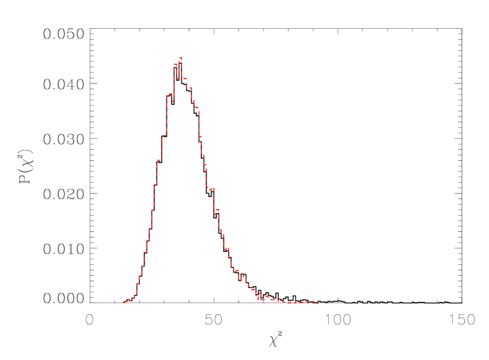
Figure 1: Distribution of $\chi^{2}$ values computed for the 10,000 simulations by solving for ${\cal N}$ and $u$ analytically using the method described in the text (dashed line), and numerically using Brent’s root-finding algorithm (solid line). Both histograms have a bin size of one and are normalized to integrate to one.

Each time a $\chi^{2}$ is calculated we solve for the normalization ${\cal N}$ and calibration factor $u$ that simultaneously minimize $\chi^{2}$. Because we did not find a closed-form analytical solution to the minimization of equation (1) with respect to ${\cal N}$ and $u$, and a numerical minimization would have been computationally prohibitive, we used the following approximation. We assume that equation (1) is well approximated by

$${\chi^{2}}\simeq\sum_{i,j}(uC_{i}^{d}-{\cal N}C_{i}^{t}){\bf\sf F}_{ij}(uC_{j}^{d}-{\cal N}C_{j}^{t})+{{(u-1)^{2}}\over{\sigma_{u}^{2}}}.$$ (4)

Where the Fisher matrix ${\bf\sf F}_{ij}$ for the $C_{i}^{d}$ quantities, is related to ${\bf\sf M}_{ij}$ by

$${\bf\sf M}_{ij}={\bf\sf F}_{ij}(C_{i}^{d}+x_{i})(C_{j}^{d}+x_{j}).$$ (5)

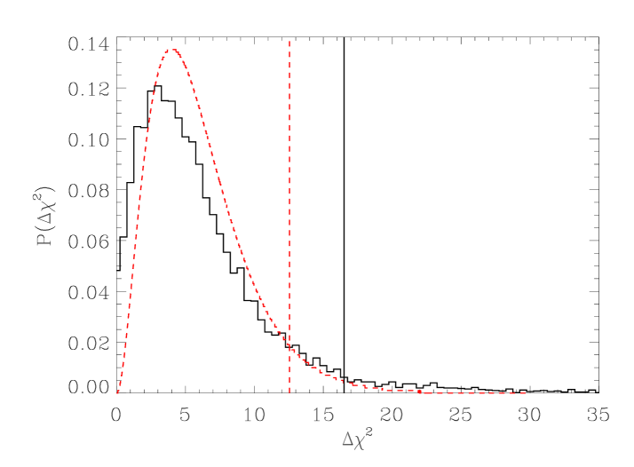
Figure 2: The histogram gives the $\Delta\chi^{2}$ distribution for the entire six-dimensional parameter space from 10,000 simulations of the COBE and MAXIMA-1 band powers. The dashed curve is the standard $\chi^{2}$ distribution for six degrees of freedom. The vertical solid line (vertical dashed line) is $\Delta\chi^{2}=16.5\,(12.8)$, which corresponds to the 95% $\Delta\chi^{2}$ threshold for the histogram (standard $\chi^{2}$ distribution). The histogram has a bin size of 0.5, and is normalized to integrate to one.

Minimization of equation (4) with respect to ${\cal N}$ and $u$ gives two coupled equations which we solve for $u$ by assuming that ${\cal N}=1$. We then use that value of $u$ to solve for ${\cal N}$. We compared this approximate solution to a rigorous numerical minimization of equation (1) for 10,000 cases and found an RMS fractional error of less than 1.5% (see Figure 1). Once the factors ${\cal N}$ and $u$ have been determined using equation (4), the exact equation (1) is used to find the value of $\chi^{2}$.

4 Determining Confidence Levels

4.1 Frequentist Confidence Intervals

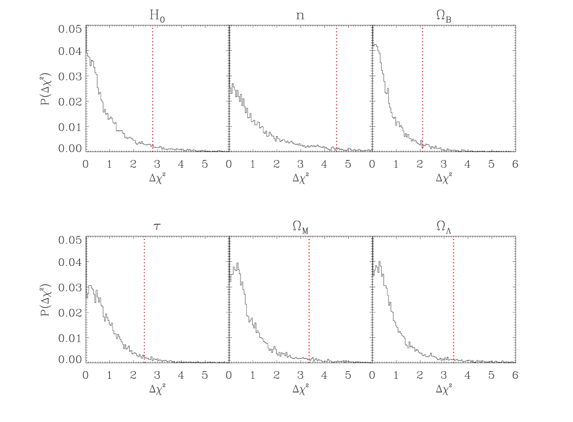
Figure 3: Simulated one-dimensional $\Delta\chi^{2}$ distributions for all the parameters in the database. The vertical dotted lines correspond to the 95% $\Delta\chi^{2}$ threshold level; numerical values are given in Table 1. Each histogram has a bin size of $0.05$ and is normalized to integrate to one. The 95% threshold for a standard $\chi^{2}$ distribution with one degree of freedom is $\chi^{2}=3.8$.

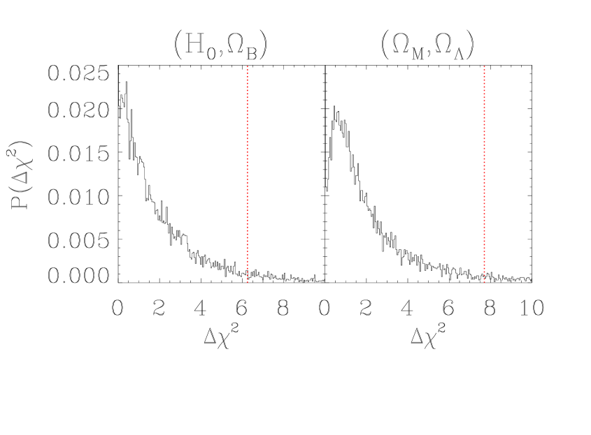
Figure 4: Simulated two-dimensional $\Delta\chi^{2}$ distributions in the $(H_{0},\Omega_{\rm B})$ and $(\Omega_{\rm M},\Omega_{\Lambda})$ planes. The vertical dotted lines correspond to the 95% $\Delta\chi^{2}$ cutoff level, which are 6.25 and 7.70 for $(H_{0},\Omega_{\rm B})$ and $(\Omega_{\rm M},\Omega_{\Lambda})$ respectively. Each histogram has a bin size of $0.05$ and is normalized to integrate to one. The 95% threshold for a standard $\chi^{2}$ distribution with two degrees of freedom is $\chi^{2}=6$.

Let ${\bf a}$ denote a vector of parameters in our six-dimensional parameter space, and ${\bf a}_{\rm true}$ be the unknown true values of the cosmological parameters that we are trying to estimate. By minimizing $\chi^{2}$ we find that the best-fitting model to the MAXIMA-1 and COBE data has the following parameters ${\bf{a}}_{0}$: $(H_{0},\Omega_{\rm B},\Omega_{\rm M},\Omega_{\Lambda},n,\tau)=(60,.075,.7,.2,1,0)$. This model gives a $\chi^{2}=36$, which is an excellent fit to 38 data points. We define

$$\Delta\chi^{2}({\bf a})\equiv\chi^{2}({\bf a})-\chi^{2}({\bf{a}}_{0}),$$ (6)

where the first term on the right hand side is a $\chi^{2}$ of the data with a model in the database, and the second is a $\chi^{2}$ of the data with the best-fitting model. To quantify the probability distribution of the data as a function of the parameters we choose a threshold $\Theta$, and define ${\cal R}$ to be the region in parameter space such that $\Delta\chi^{2}\leq\Theta$. ${\cal R}$ is a confidence region at level $\alpha$ if there is a probability $\alpha$ that ${\cal R}$ contains the true cosmological parameters ${\bf a_{\rm true}}$. In other words, if many vectors ${\bf{a}}_{0(j)}$ and regions ${\cal R}_{j}$ are generated by repeating the experiment many times, a fraction $\alpha$ of the ensemble of ${\cal R}_{j}$ would contain ${\bf a_{\rm true}}$. Since the $\Delta\chi^{2}$ statistic may not be $\chi^{2}$ distributed, we use simulations to determine its probability distribution as a function of the cosmological parameters.

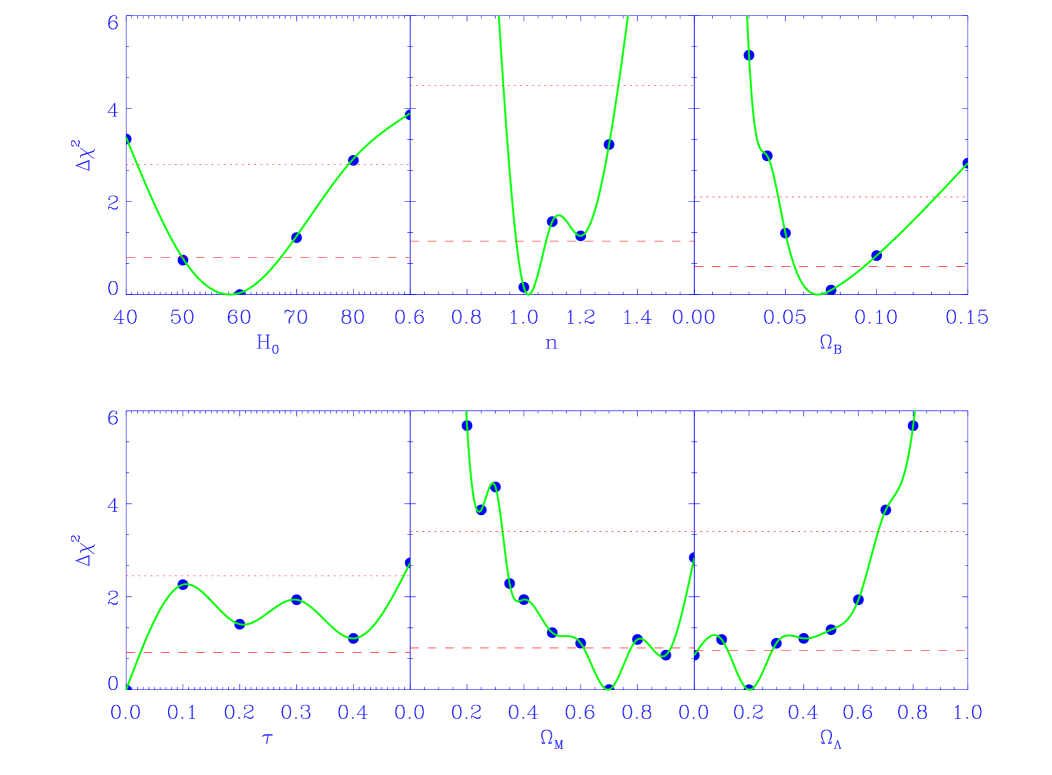
Figure 5: $\Delta\chi^{2}$ calculated with the MAXIMA-1 and COBE data as a function of parameter value for each of the parameters in the database. Solid circles show grid points in parameter space, and the solid lines were obtained by interpolating between grid points. The parameter values where the solid line intercepts the dashed (dotted) line corresponds to the 68% (95%) frequentist confidence region.

The simulations mimic 10,000 independent observations of the CMB by the MAXIMA-1 and COBE experiments. The CMB is assumed to be characterized by the MAXIMA-1 and COBE best estimate for the cosmological parameters, ${\bf{a}}_{0}$. Applying the equivalent of equation (6) [see equations (7) and (8)] for each of the simulations gives a set of 10,000 values $\Delta\chi^{2}_{j}$ ($j=1,...,10^{4}$), and by histogramming these values we associate threshold levels $\Theta$ with probabilities $\alpha$. This relation between $\Theta$ and $\alpha$ is applied to the distribution of $\Delta\chi^{2}$ that is calculated using equation (6) to determine a frequentist confidence interval ${\cal R}$ on the cosmological parameters. Note that our procedure assumes that the probability distribution of $\Delta\chi^{2}$ around ${\bf{a}}_{0}$ closely mimics the probability distribution of $\Delta\chi^{2}$ around ${\bf a_{\rm true}}$. This is a standard assumption in frequentist analyses [Press et al. 1992]. The alternative approach of determining the probability distribution around each grid point in parameter space is computationally prohibitive.

Because finding the best-fitting band powers from a time stream or even a sky map is computationally expensive [Borrill 1999], we perform 10,000 simulations of the quantities $Z_{i}^{d}$, which are related to the band powers $C_{\ell}$ as defined in equation (3). We assume that the $Z_{i}^{d}$ are Gaussian-distributed [Bond, Jaffe, & Knox 2000] and we discuss and justify this assumption in Appendix A.

The quantities $Z_{i(j)}^{d}$, where $j$ denotes one of the 10,000 simulations, are drawn from two multivariate Gaussian distributions that represent the MAXIMA-1 (10 data points) and COBE (28 data points) band powers. The means of the distributions are the $Z_{i}^{t}$ quantities as determined by ${\bf a_{0}}$, and the covariances are taken from the data. Each of the $Z_{i{(j)}}^{d}$ is thus a vector with 38 elements representing an independent observation of a universe with a set of cosmological parameters $\bf{a_{0}}$ . We include uncertainty in the calibration and beam-size of the MAXIMA-1 experiment by multiplying the MAXIMA band-powers by two Gaussian random variables. The calibration random variable has a mean of one and standard deviation of 0.08, and the beam-size random variable has a mean of one and a variance that is $\ell$-dependent [Hanany et al. 2000, Wu et al. 2001b]. For each simulation $j$ the entire database of cosmological models is searched for the vector of parameters ${\bf{a}}_{0(j)}$ which minimizes $\chi^{2}$, and we calculate $\Delta\chi^{2}_{j}$:

$$\Delta\chi^{2}_{j}=\chi^{2}_{j}({\bf a}_{0})-\chi^{2}_{j}({\bf a}_{0(j)}).$$ (7)

The first and second terms on the right hand side are the $\chi^{2}$ of simulation $j$ with the model $\bf{a_{0}}$, and of simulation $j$ with its best-fitting model, respectively. A normalized histogram of $\Delta\chi^{2}_{j}$ for all 10,000 simulations is shown in Figure 2 and gives the probability distribution of $\Delta\chi^{2}$ over the six-dimensional parameter space. The 95% threshold is $\Delta\chi^{2}=16.5$, that is, 95% of the probability is contained in the range $0\leq\Delta\chi^{2}\leq 16.5$. Figure 2 also shows a standard $\chi^{2}-$distribution with six degrees of freedom and its associated 95% threshold level. The difference between the results of the simulations and the standard $\chi^{2}$ distribution is attributed to the non-linear dependence of the models on the parameters and minimizing $\chi^{2}$ over ${\cal N}$ and $u$.

Contour levels in the six-dimensional parameter space that are provided by different thresholds of the distribution of $\Delta\chi_{j}^{2}$ cannot be used to set confidence intervals on any individual parameter. To find a confidence interval for a single parameter $p$ we compute the probability distribution $\Delta\chi^{2}_{(p)}$ in the following way. We search the database for the model that minimizes the $\chi^{2}$ with simulation $j$ under the condition that $p$ is fixed at its value in $\bf{a_{0}}$, and for the model that minimizes the $\chi^{2}$ with simulation $j$ with no restrictions on the parameters. We compute

$$\Delta\chi^{2}_{(p)}=\chi^{2}_{j}({\bf a}_{(p)})-\chi^{2}_{j}({\bf a}_{0(j)}),$$ (8)

where ${\bf a}_{(p)}$ is the vector of parameters that minimize $\chi^{2}$ subject to the constraint that $p$ is fixed. A histogram of $\Delta\chi^{2}_{(p)}$ provides the necessary distribution. The one-dimensional distributions for all six parameters in the database are shown in Figure 3. Generalization of this process for finding the probability distribution for any subset of parameters is straightforward. The two-dimensional $\Delta\chi^{2}$ distributions in the $(H_{0},\Omega_{\rm B})$ and $(\Omega_{\rm M},\Omega_{\Lambda})$ planes are shown in Figure 4 and the corresponding 95% thresholds are $\Delta\chi^{2}=6.25$ and $\Delta\chi^{2}=7.70$, respectively.

Using the simulated one- and two-dimensional probability distributions of $\Delta\chi^{2}$ we set 68% and 95% threshold levels on the distribution of $\Delta\chi^{2}$ that are calculated using the data and the database of models, i.e. the one calculated from equation (6), and we determine corresponding confidence intervals on the cosmological parameters. Figures 5, 6, and 7 give the association between $\Delta\chi^{2}$ and cosmological parameter values for each of the parameters in the database and in the $(H_{0},\Omega_{\rm B})$ and $(\Omega_{\rm M},\Omega_{\Lambda})$ planes.

Figure 6: Two-dimensional frequentist confidence regions in the ($\Omega_{\rm M},\Omega_{\Lambda}$) plane. The red, orange, and yellow regions correspond to the 68%, 95%, and 99% confidence regions respectively. The dashed line corresponds to a flat universe, $\Omega=\Omega_{\rm M}+\Omega_{\Lambda}=1$.

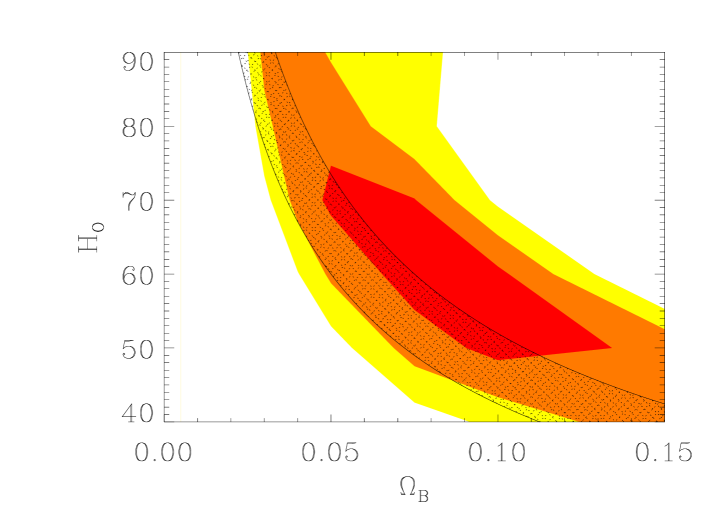
Figure 7: Two-dimensional frequentist confidence regions in the ($H_{0},\Omega_{\rm B}$) plane. The red, orange, and yellow regions correspond to the 68%, 95%, and 99% confidence regions respectively. Standard calculations from big bang nucleosynthesis and observations of ${{D}/{H}}$ predict a 95% confidence region of $\Omega_{\rm B}h^{2}=0.021{+0.006\atop-0.003}$ [Cyburt, Fields, & Olive 2001a], indicated by the shaded region.

4.2 Bayesian Credible Regions

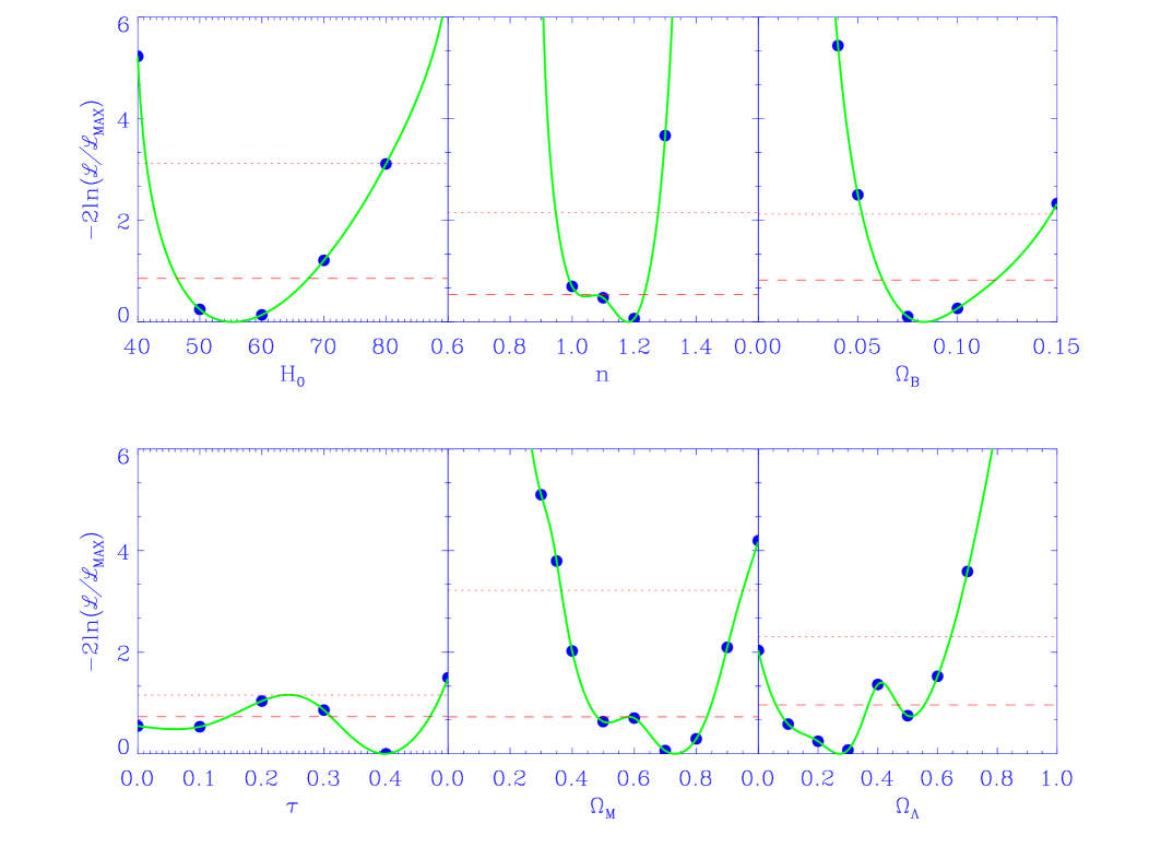
Figure 8: Bayesian likelihood functions for each of the parameters in the database. Solid circles show grid points in parameter space, while the solid lines were obtained by interpolating between grid points. The parameter values where the solid line intercepts the dashed (dotted) line corresponds to the 68% (95%) Bayesian credible regions.

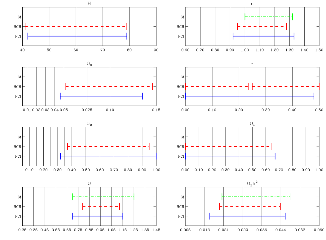
Figure 9: A comparison of the 95% frequentist confidence intervals (FCI, solid line), Bayesian credible regions (BCR, dashed line), and maximization regions (M, dashed dot line) for the parameters in the database, and for $\Omega$ and $\Omega_{\rm B}h^{2}$.

According to Bayes’s theorem the probability of a model given the data, the posterior probability, is proportional to the product of the likelihood ${\cal L}\left({\bf a}\right)=\exp(-{1\over 2}\chi^{2}({\bf a}))$ and a prior probability distribution of the parameters. If the prior is constant, as we shall assume, then the posterior probability is directly proportional to the likelihood function. To set a Bayesian credible region for any parameter or subset of parameters of interest we calculate the likelihood ${\cal L}({\bf a})$ for all models in the database, assume a flat prior probability distribution for all parameters, and integrate the likelihood over the remaining parameters. The 95% credible region is the region that encloses 95% of the probability. The likelihood functions for each parameter in the database are shown in Figure 8.

5 Results

The 95% frequentist confidence intervals and Bayesian credible regions for each parameter in the database are given in Table 1 and Figure 9.

We found that the optical depth to last scattering $\tau$ was degenerate with other parameters in the database, mostly with the spectral index of the primordial power spectrum $n$. Because of this degeneracy the 95% confidence interval of $\tau$ covers nearly the entire range of values considered, and the 95% credible region is disjoint.

95% Confidence Regions
Parameter	$\Delta\chi^{2}_{(95\%)}$	frequentist	Bayesian	Balbi et al.
$H_{0}$	2.80	[42,79]	[41,79]	—
$n$	4.50	[0.92,1.33]	[0.95,1.28]	[1.00,1.32]
$\Omega_{\rm B}$	2.10	[0.046,0.135]	[0.052,0.146]	—
$\tau$	2.45	$\leq 0.48^{\rm a}$	—	—
$\Omega_{\rm M}$	3.40	$\geq 0.32^{\rm a}$	[0.37,0.95]	—
$\Omega_{\Lambda}$	3.40	$\leq 0.67^{\rm a}$	$\leq 0.64^{\rm a}$	—
$\Omega$	5.1	[0.70,1.15]	[0.79,1.12]	[0.70,1.25]
$\Omega_{\rm B}h^{2}$	5.6	[0.015,0.046]	[0.019,0.044]	[0.020,0.048]
a: Sets only upper or lower limits on parameter

Table 1: A comparison of Bayesian, frequentist and maximization 95% confidence intervals. The table also gives the 95% $\Delta\chi^{2}$ thresholds from the simulations. Maximization confidence intervals are taken from Balbi et al. (2000); they do not give confidence intervals for all the parameters.

The 95% confidence intervals and credible regions for $H_{0}$, $\Omega_{\rm B}$, $\Omega_{\rm M}$ and $\Omega_{\Lambda}$ include most of the parameter values because the angular power spectrum of the CMB is not very sensitive to any one of them alone. It is more sensitive to the combination $\Omega_{\rm B}h^{2}$, and to the total energy density parameter $\Omega=\Omega_{\rm M}+\Omega_{\Lambda}$. To set confidence intervals and credible regions for these new parameters we formed all possible combinations of $\Omega$ and $\Omega_{\rm B}h^{2}$ in our database and binned them in the following bins for $\Omega_{\rm B}h^{2}$: {$0.00500$,$0.0129$,$0.0207$,$0.0286$,$0.0364$,$0.0442$, $0.0521$,$0.0600$}, and for $\Omega$: {$0.25$,$0.35$,$0.45$,$0.55$,$0.65$,$0.75$, $0.85$,$0.95$,$1.05$,$1.15$,$1.25$,$1.35$,$1.45$}. The center value in each bin is considered a new database grid point. We repeat the process used to find the 95% $\Delta\chi^{2}$ threshold for $\Omega_{\rm B}h^{2}$ and $\Omega$, treating them as one-dimensional parameters. We also calculate the appropriate integrated likelihood functions. Table 1 lists the 95% $\Delta\chi^{2}$ threshold, confidence interval, and credible regions for $\Omega$ and $\Omega_{\rm B}h^{2}$.

We determined the frequentist and Bayesian central values for $n$, $\Omega_{\rm B}h^{2}$ and $\Omega$, the parameters to which the CMB power spectrum is most sensitive. In the frequentist approach the central value of a parameter is the value given by the best-fitting model, and the Bayesian central value is the maximum marginalized likelihood parameter value. The frequentist and Bayesian analyses give respectively a value of $\Omega=0.89{+0.26\atop-0.19}$ and $0.98{+0.14\atop-0.19}$, $\Omega_{\rm B}h^{2}=0.026{+0.020\atop-0.011}$ and $0.029{+0.015\atop-0.010}$, and $n=1.02{+0.31\atop-0.10}$ and $1.18{+0.10\atop-0.23}$, all at the 95% confidence level.

6 Discussion

A comparison of the frequentist confidence intervals and the Bayesian credible regions is shown in Figure 9. We have also included the results of Balbi et al. (2000), who set parameter confidence intervals using the same data set considered in this paper but use maximization rather than marginalization of the likelihood function. In this method the likelihood function for a parameter is determined by finding the maximum of the likelihood ${\cal L}({\bf a})$ as a function of the remaining parameters. When ${\cal L}({\bf a})$ is Gaussian maximization and marginalization are equivalent.

The central values and the widths of confidence intervals derived from all three methods give consistent results within about 15% and 30% respectively. A closer examination suggests, however, that frequentist confidence intervals are somewhat broader than the Bayesian ones. For five out of eight parameters ($n$, $\Omega_{\rm M}$, $\Omega_{\Lambda}$, $\Omega$, and $\Omega_{\rm B}h^{2}$) the frequentist confidence intervals are somewhat larger than the Bayesian credible regions, and for $H_{0}$ the intervals are nearly identical. For the three parameters for which we have results from all three methods the Bayesian intervals are either the narrowest ($\Omega_{\rm B}h^{2}$ and $\Omega$) or identical to maximization ($n$). Also, we find that the 99% frequentist confidence intervals are somewhat wider than the 99% Bayesian credible regions for every parameter considered except $\Omega_{\rm B}$.

Despite this pattern which suggests that a frequentist analysis gives broader confidence intervals, it is difficult to claim such a pattern conclusively. Furthermore, it is not useful to quantify the pattern exactly because the difference in confidence interval widths is usually within one parameter grid point. Much finer gridding and hence a much larger database would be necessary to claim such a pattern with high confidence. A larger database would also provide a more accurate determination of the $\Delta\chi^{2}$ functions in Figure 5, and the likehood functions in Figure 8. However, a larger database would have been computationally prohibitive.

The difference between the confidence interval and credible region for the baryon density $\Omega_{\rm B}h^{2}$ is of some interest. Maximization [Balbi et al. 2000] and Bayesian [Jaffe et al. 2001] analyses of the MAXIMA-1 and COBE data gave consistency between $\Omega_{\rm B}h^{2}$ from CMB measurements and a value of 0.021 from some determinations of ${{D}/{H}}$ from quasar absorption regions [O’Meara et al. 2001] only at the edge of the 95% intervals. This was interpreted as a tension between CMB measurements and either deuterium abundance measurements or calculations of BBN [Tegmark & Zaldarriaga 2000, Griffiths, Silk & Zaroubi 2000, Cyburt, Fields, & Olive 2001b]. A value of 0.021 for $\Omega_{\rm B}h^{2}$ is consistent with the frequentist confidence interval at a level of 75%, an agreement at a confidence of just over $1\sigma$. Recent analysis of new CMB data is consistent with a value of $\Omega_{\rm B}h^{2}=0.021$ within a $1\sigma$ level [Pryke et al. 2001, Netterfield et al. 2001].

The comparison between the Bayesian- and frequentist-based analyses raises the question of whether agreement at the level observed was in fact expected. The Bayesian and frequentist approaches to parameter estimation are conceptually quite different. A Bayesian asks how likely a parameter is to take on any particular value, given the observed data. A frequentist, on the other hand, asks how likely the given data set is to have occurred, given a particular set of parameters. Since the two questions are completely different, there is no guarantee that they will yield identical answers in general. In certain specific situations Bayesian and frequentist approaches can be shown to yield the same results. For example, in the particular case of Gaussian-distributed data with uniform priors and linear dependence of the predictions on the parameters, the two approaches coincide. However, these hypotheses (particularly the last one) do not apply to the case we are considering.

Bayesian and frequentist methods also coincide asymptotically, i.e. in the limit as the number of independent data points tends to infinity (Ferguson 1996). In that limit, all confidence regions would be small in comparison to the prior ranges of the parameters, and the Bayesian prior-dependence would become negligible. CMB data are clearly not yet in this limit.

7 Acknowledgments

Computing resources were provided by the University of Minnesota Supercomputing Institute. We acknowledge the use of CMBFast. MA, SH, and RS acknowledge support from NASA Grant NAG5-3941. JHPW and AHJ acknowledge support from NASA LTSA Grant no. NAG5-6552 and NSF KDI Grant no. 9872979. BR and CDW acknowledge support from NASA GSRP Grants no. S00-GSRP-032 and S00-GSRP-031. EFB acknowledges support from NSF grant AST-0098048. The work of KAO was supported partly by DOE grant DE–FG02–94ER–40823. PGF acknowledges support from the Royal Society. MAXIMA is supported by NASA Grant NAG5-4454.

Appendix A Probability Distribution of the Experimental Data

BJK have shown that the band-powers are well-approximated by an offset log-normal distribution. Specifically, they showed that the probability distribution $p(Z_{i}^{d}\ |\ Z_{i}^{t})$ is approximately Gaussian as a function of $Z_{i}^{t}$. Furthermore, it is possible to compute the covariance matrix of these Gaussian random variables.

The calculation in BJK was performed in a Bayesian framework. For the frequentist analysis we need to know the probability distribution $p(Z_{i}^{d}\ |\ Z_{i}^{t})$ as a function of $Z_{i}^{d}$, not as a function of $Z_{i}^{t}$. (This is the heart of the difference between the two approaches: for a Bayesian the data are fixed and the theoretical quantities are described probabilistically; a frequentist treats the data as a random variable for fixed values of the parameters.) We therefore make the ansatz that the probability distribution is Gaussian in $Z_{i}^{d}$ as well.

	Small Map	Large Map
${\bf\sf M}_{00}$	$1.5\times 10^{7}\pm 1.2\times 10^{6}$	$1.2\times 10^{8}\pm 2.8{\bf\times}10^{6}$
${\bf\sf M}_{01}$	$2.0\times 10^{6}\pm 7.4\times 10^{4}$	$4.5\times 10^{6}\pm 7.9\times 10^{4}$
${\bf\sf M}_{11}$	$2.1\times 10^{7}\pm 2.6\times 10^{6}$	$1.2\times 10^{8}\pm 7.3\times 10^{6}$

Table 2: The average values with sample standard deviations of the marginalized $Z_{l}$ weight matrix entries for both large and small map simulations. The large map simulations were based on pointing from the MAXIMA-1 $8^{\prime}$ map, and the small map pointing was based on a center patch of the map. Units are dimensionless MADCAP units

If the $Z_{i}^{d}$ are indeed Gaussian distributed, then the entries of the weight matrix ${\bf\sf{M}}$ (inverse covariance matrix) should be exactly the same for independent observations of universes which have the same underlying CMB power spectrum. We test the assumption of Gaussianity using simulations. We generate CMB maps using a particular cosmological model, compute the power spectrum and ${\bf\sf M}$ for each map and assess the variance in the entries of ${\bf\sf M}$ between simulations. A small variance would indicate that the assumption that the $Z_{i}^{d}$ are Gaussian-distributed is adequate.

We generated 100 small-area and 30 large-area map simulations using ${\bf a}_{0}$ as the cosmological model and computed the ${\bf\sf M}$ matrix for each map (the number of simulations is limited by the computational resources required to estimate the power spectrum for each map). The small- and large-area maps contain 542 and 5972 $8^{\prime}$ pixels respectively. Power spectra and $Z_{l}$ were computed in four bins of $l=${2,300},{301,600},{601,900},{901,1500}, and ${\bf\sf M}$ was obtained by marginalizing over the first and last bins. The results are summarized in Table 21. The average value of the diagonal entries increases for the larger-area maps because for those the band powers have smaller errors and hence larger values in the weight matrix. The percent fluctuation in the matrix entries of the large-area maps are 2% for the first diagonal entry, 6% for the second diagonal entry, and 2% for the off diagonal entries. We consider this variance to be small enough to indicate that the assumption of Gaussianity of the $Z_{i}^{d}$ is acceptable. We also note that the variance of the matrix elements decreases as a function of increasing map size. If such a trend continues to maps of the size of the MAXIMA-1 map, which has more than 15,000 pixels, then the assumption of Gaussianity is well satisfied.

References

- [Balbi et al. 2000] Balbi A. et al., 2000, ApJ, 545, L1, Erratum, 2001, 558, L145
- [Bond, Jaffe, & Knox 2000] Bond J.R., Jaffe A.H., & Knox L., 2000, ApJ, 533, 19
- [Borrill 1999] Borrill J., 1999, in EC-TMR Conference Procedings 476, 3K Cosmology, ed. L. Maiani, F. Melchiorri, & N. Vittorio (Woodbury, New York: AIP), 224
- [Bunn et al. 1994] Bunn E., White M. Srednicki M., & Scott D., 1994, ApJ 429, 1
- [Cyburt, Fields, & Olive 2001a] Cyburt R., Fields B., Olive K.A., 2001, NewA, 6, 215C
- [Cyburt, Fields, & Olive 2001b] Cyburt R., Fields B., & Olive K.A., 2001, preprint, astro-ph/0105397
- [de Bernardis el al. 2000] de Bernardis P. et al., 2000, Nature, 404, 955-959
- [Douspis, Barlett, & Blanchard 2001] Douspis M., Bartlett J.G., & Blanchard A., 2001, A&A, 379, 1
- [Ferguson 1996] Ferguson T.M., 1996, A Course in Large Sample Theory. Chapman and Hall, Baton Raton, FL
- [Gawiser 2001] Gawiser E., 2001, preprint, astro-ph/0105010
- [Górski, Stompor, & Juszkiewicz 1993] Górski K.M., Stompor R., & Juszkiewicz R., 1993, ApJ, 410, L1
- [Górski et al. 1996] Górski K.M. et al., 1996, ApJ, 464, L11
- [Griffiths, Silk & Zaroubi 2000] Griffiths L.M., Silk J., & Zaroubi S., 2000, ApJ, 553, L5
- [Halverson et al. 2001] Halverson N.W. et al., 2001, preprint, astro-ph/0104489
- [Hanany et al. 2000] Hanany S. et al., 2000, ApJ, 545, L5
- [Hivon et al. 2001] Hivon E., Górski K.M., Netterfield C.B., Crill B.P., Prunet S., & Hansen F., 2001, preprint, astro-ph/0105302
- [Jaffe et al. 2001] Jaffe A.H. et al., 2001, Phys. Rev. Lett., 86, 3475
- [Lange et al. 2001] Lange A.E. et al., 2001, Phys. Rev. D, 63, 042001
- [Lee et al. 1999] Lee, A.T. el al., 1999, in EC-TMR Conference Procedings 476, 3K Cosmology, ed. L. Maiani, F. Melchiorri, & N. Vittorio (Woodbury, New York: AIP), 224
- [Lee et al. 2001] Lee A.T. et al., 2001, ApJ, 561, L1
- [Miller et al. 2001] Miller A. et al., 2001, preprint, astro-ph/0108030
- [Netterfield et al. 2001] Netterfield C.B. et al., 2001, preprint, astro-ph/0104460
- [O’Meara et al. 2001] O’Meara J.M., Tytler D., Kirkman D., Suzuki N., Prochaska J., Lubin D., & Wolfe A., 2001, ApJ, 522, 718
- [Padmanabhan & Sethi 2000] Padmanabhan T. & Sethi S. K., 2000, preprint, astro-ph/0010309
- [Press et al. 1992] Press W., Teukolsky S., Vetterling W., & Flannery B., 1992, Numerical Recipes in C, 15.6. Cambridge University Press
- [Pryke et al. 2001] Pryke C. et al., 2001, preprint, astro-ph/0104490
- [Santos 2001] Santos M.G. et al., 2001, preprint, astro-ph/0107588
- [Seljak & Zaldarriaga 1996] Seljak U., & Zaldariagga M., 1996, ApJ, 469, 437
- [Stompor et al. 2001] Stompor R. et al., 2001, ApJ, 561, L7
- [Stompor & Górski 1994] Stompor R. & Górski K.M., 1994, ApJ, 422, L41
- [Tegmark & Zaldarriaga 2000] Tegmark M., & Zaldarriaga M., 2000, Phys. Rev. Lett., 85, 2240
- [Wang, Tegmark, & Zaldarriaga 2001] Wang X., Tegmark M., & Zaldarriaga M., 2001, preprint, astro-ph/0105302
- [Wu et al. 2001a] Wu J.H.P. et al., 2001a, Phys. Rev. Lett., 87, 251303
- [Wu et al. 2001b] Wu J.H.P. et al., 2001b, ApJS, 132, 1