THE FATE OF THE FIRST GALAXIES. I.
SELF-CONSISTENT COSMOLOGICAL SIMULATIONS WITH RADIATIVE TRANSFER

Abstract

In cold dark matter (CDM) cosmogonies, low-mass objects play an important role in the evolution of the universe. Not only are they the first luminous objects to shed light in a previously dark universe, but, if their formation is not inhibited by their own feedback, they dominate the galaxy mass function until redshift $z\sim 5$. In this paper we present and discuss the implementation of a 3D cosmological code that includes most of the needed physics to simulate the formation and evolution of the first galaxies with a self-consistent treatment of radiative feedback. The simulation includes continuum radiative transfer using the “Optically Thin Variable Eddington Tensor” (OTVET) approximation and line-radiative transfer in the H₂ Lyman-Werner bands of the background UV radiation. We include detailed chemistry for H₂ formation/destruction, molecular and atomic cooling/heating processes, ionization by secondary electrons, and heating by Ly$\alpha$ resonant scattering.

We find that the first galaxies (“small-halos”) are characterized by bursting star formation, self-regulated by a feedback process that acts on cosmological scales. The mass in stars produced by these objects can exceed the mass in stars produced by normal galaxies; therefore, their impact on cosmic evolution cannot be neglected. The main focus of this paper is on the methodology of the simulations, and we only briefly introduce some of the results. An extensive discussion of the results and the nature of the feedback mechanism are the focus of a companion paper.

1 Introduction

In the last five years, precise observations of the cosmic microwave background (CMB), Ly$\alpha$ forest, galaxy clusters, and large scale structure have produced a large amount of data that strongly constrain the standard cosmological model. Until now, despite some unsolved problems (Moore, 1994; Klypin et al., 1999; Navarro & Steinmetz, 2000), cold dark matter (CDM) cosmogonies remain the most predictive cosmological models. In CDM cosmogonies, the large galaxies that we observe today are the result of the mergers of a large number of small and faint galaxies (dwarf galaxies). The number of dwarf galaxies observed in the local universe is larger than the number of normal galaxies but, today, they account for only a small fraction of the mass in collapsed objects. About 12 billion years ago, galaxies with the mass of our Milky Way were extremely rare, and the universe was filled with objects similar to dwarf spheroidal galaxies.

How small can a galaxy be? Or how small can a protogalaxy be in order to be able to form stars? A necessary condition for star formation is that the gas in the protogalaxy must cool to a temperature lower than the virial temperature of the halo in a Hubble time. If the dark matter (DM) mass is $M_{DM}\lower 2.15277pt\hbox{$\;\buildrel>\over{\sim}\;$}10^{8}$ M_⊙, the gas in the protogalaxy (a so-called “large-halo” protogalaxy) cools by H i emission lines because the virial temperature of the halo is $T_{vir}\lower 2.15277pt\hbox{$\;\buildrel>\over{\sim}\;$}10^{4}$ K. But if $M_{DM}\lower 2.15277pt\hbox{$\;\buildrel<\over{\sim}\;$}10^{8}$ M_⊙ and the protogalaxy is of primordial composition, the gas cannot cool ($T_{vir}\lower 2.15277pt\hbox{$\;\buildrel<\over{\sim}\;$}10^{4}$ K) unless molecular hydrogen (H₂) is present. We call such an object a “small-halo” protogalaxy. During the virialization process, the gas is partially ionized ($x_{e}\sim 10^{-4}$) and heated to the virial temperature by shocks. Free electrons can be captured by neutral hydrogen (H i ) to produce H^-, which is the main catalyst for H₂ formation in a gas of primordial composition (Lepp & Shull, 1984). The chemical reaction H i $+{\rm H}^{-}\rightarrow{\rm H}_{2}+e^{-}$ produces enough H₂ ($x_{H_{2}}\sim 10^{-4}$) to allow the formation of galaxies as small as $M_{DM}\sim 10^{5}$ M_⊙ at $z\sim 30$, i.e., with virial temperature $T_{vir}\sim 360$ K (Tegmark et al., 1997; Abel, Bryan, & Norman, 2000).

“Small-halo” objects are thought to be the first galaxies formed in the universe and, if their formation is not inhibited by feedback, they should account for the bulk of mass in stars until reionization at $z\sim 6$. In Figure 1 we show the fraction of collapsed (virialized) DM as a function of the DM halo mass at $z=24,19,16,9,5,3,0$ calculated with the Press-Schechter formula (Press & Schechter, 1974). The inserted table shows the fraction of the collapsed mass in “small-halo” objects ($T_{vir}<10^{4}$ K), normal galaxies (“large-halo” objects with $10^{4}~{}{\rm K}\leq T_{vir}\leq 10^{6}$ K), and clusters ($T_{vir}>10^{6}$ K). The last column in the table shows the ratio of the collapsed mass of the “small-halo” to the “large-halo” objects. The hexagons, squares, and triangles show the mass of 1 $\sigma$, 2 $\sigma$, and 3 $\sigma$ perturbations of the initial density field, respectively. “Small-halo” objects are the dominant fraction of the DM collapsed mass before redshift $z\sim 9$, and they remain an important fraction of the DM collapsed mass until redshift $z\sim 5$.

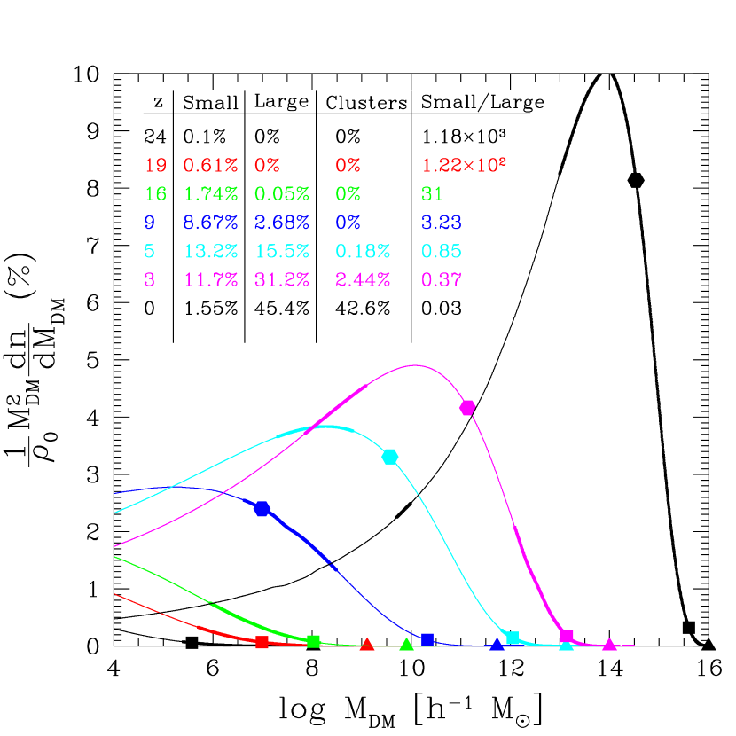
Figure 1: Fraction of collapsed (virialized) DM as a function of the DM halo mass at $z=25$, calculated using the Press-Schechter formalism. The inserted table shows the fraction of the collapsed mass in “small-halo” protogalaxies ($T_{vir}<10^{4}$ K), normal galaxies (“large-halo” protogalaxies with $10^{4}{\rm K}\leq T_{vir}\leq 10^{6}$ K), and clusters ($T_{vir}>10^{6}$ K). The last column in the table shows the ratio of the collapsed mass of “small-halo” to “large-halo” protogalaxies. “Small-halo” objects are an important fraction of the DM collapsed mass until redshift $z\sim 5$. Each curve has two thick portions: the thick section on the left shows “small-halo” objects, and the thick section on the right, clusters. In between, according to our definition, are “large-halo” objects.

Competing feedback effects determine the fate of “small-halo” objects. Radiative feedback regulates the formation and destruction of H₂ in the protogalaxies. Mechanical and thermal feedback from supernova (SN) explosions could blow away the interstellar medium of “small-halo” objects, produce H₂ (Ferrara, 1998), or destroy H₂. In this paper, we focus on radiative feedback processes. From the first works on this subject (Haiman, Rees, & Loeb, 1997, 2000; Ciardi et al., 2000; Machacek, Bryan, & Abel, 2001), the negative feedback from the background in the H₂ Lyman-Werner bands was thought to be the main process that regulates the formation of “small-halo” objects. The background in the Lyman-Werner bands dissociates H₂ through the two-step Solomon process, suppressing or delaying the formation of “small-halo” objects. But there are also positive feedback processes that can enhance the formation rate of H₂ (Mac Low & Shull, 1986; Shapiro & Kang, 1987; Haiman, Rees, & Loeb, 1996; Ferrara, 1998; Oh, 2001; Ricotti, Gnedin, & Shull, 2001). It is not trivial to determine which feedback prevails by means of semi-analytic models. Are “small-halo” objects able to form and survive the negative feedback effect of the dissociating background, or is their number drastically suppressed? Are “small-halo” objects numerous enough to have some effect on the subsequent evolution of the IGM? In this work we try to answer these questions, using self-consistent 3D cosmological simulations with radiative transfer.

We present our results in two papers. This first paper focuses on the implementation of the code and its convergence. In Ricotti, Gnedin, & Shull (2002) (Paper II) we show and discuss the results.

The simulations we present here are the first 3D cosmological simulations that include a self-consistent treatment of galaxy formation with radiative transfer by following the evolution of DM particles, star particles, gas, and photons. We also solve the line radiative transfer for the background in the Lyman-Werner bands. A number of potentially relevant physical processes are included as well: secondary ionizations of H and He, detailed H₂ chemistry and cooling processes, heating by Ly$\alpha$ resonant scattering, H and He recombination lines, heavy element production and radiative cooling, and the spectral energy distribution (SED), $g_{\nu}$, of the stellar sources consistent with the choice of the Lyman-continuum (Lyc) escape fraction, $\langle f_{esc}\rangle$, from the resolution element of the simulation. These ingredients, together with careful convergence studies, allow us to study the formation and feedback of “small-halo” objects by means of numerical simulations. The advantage of this approach, compared to semi-analytic models, is that we make no assumptions about the physical processes that are important in the simulation, apart from sub-grid physics. We assume that, when the gas sinks below the resolution limit of the simulation, it forms stars according to the Schmidt law (see eq. [20]).

The paper is organized in the following manner. In § 2 we describe the cosmological code and the detailed physical processes simulated. In § 3 we study the convergence of the simulations, and in § 4 we summarize the features of the code and its limitations. We also provide a few examples of the results to demonstrate the power of the code to for addressing astrophysical problems.

2 The Code

The simulations presented in this paper were performed with the “Softened Lagrangian Hydrodynamics” (SLH-P³M) code described in detail in Gnedin (1995, 1996), Gnedin & Bertschinger (1996); Gnedin & Ostriker (1997), and Gnedin & Abel (2001). The code solves the system of time-dependent equations of motion of four main components: dark matter particles (P³M algorithm); gas particles (quasi-Lagrangian deformable mesh using the SLH algorithm); “star-particles” formed using the Schmidt law in resolution elements that sink below the numerical resolution of the code; and photons solved self-consistently with the radiative transfer equation in the OTVET approximation (Gnedin & Abel, 2001). We solve the line radiative transfer of the background radiation in the H₂ Lyman-Werner bands with spectral resolution $\Delta\nu/\nu=9.26\times 10^{-6}$ (i.e., 20,000 logarithmic bins in the energy range $11.2-13.6$ eV of the H₂ Lyman-Werner bands). Detailed atomic and molecular physics is included: secondary ionizations of H and He, H₂ chemistry and cooling processes, heating by Ly$\alpha$ resonant scattering, H and He recombination lines, heavy element production and radiative cooling, and galaxy spectrum consistent with the value of $\langle f_{esc}\rangle$.

For clarity, we first summarize some relevant features of the code already implemented and published. The new components of the code are described in more detail as separate subsections.

2.0.1 Radiative transfer: the OTVET approximation

The OTVET approximation is based on solving equations for the first two moments of the photon distribution function. Since the moment equations have the conservative form, the photon number and flux conservation are achieved automatically in this approximation. However, the hierarchy of moment equations is not closed at any finite level, i.e. the flux (first moment) equation contains the second moment (flux tensor), which can be reduced to the Variable Eddington tensor (the latter has a unit trace). In the OTVET approximation, the Eddington tensor is calculated in the optically thin approximation - hence the abbreviation OTVET: Optically Thin Variable Eddington Tensor approximation. Since the two moment equations can be solved very fast numerically, most of the computational time is spent in calculating the Eddington tensor, which can be done using the same algorithm used for computing gravity, in our case the Adaptive P³M.

Methodically, this approach is equivalent to separating the algorithm for calculating absorption and emission of photons from the algorithm for calculating the direction of propagation of a photon. The first part can be done rapidly and accurately by using moments of the distribution function. The second part, in a direct ray-tracing approach, will be unacceptably slow. The OTVET approximation allows us to speed up this calculation by an enormous factor without violating the accuracy of the first algorithm.

Another feature of our implementation of the OTVET approximation is the use of “effective” frequencies. Accurate computation of photoionization and photoheating rates on a logarithmically spaced mesh in the frequency space requires about 20 points per each e-folding, or about 300 frequency bins altogether. Computing the radiative transfer for each of these bins is impractical at the moment. However, since we are ultimately only interested in the integrals over the frequencies, we can speed up the calculation of the reaction rates by a factor of about 50 by adopting the following ansatz for the radiation energy density $I_{\nu}$ as a function of frequency:

$$I_{\nu}=I_{\nu,\rm OT}\exp\left(-\sum_{\alpha}\sigma_{\nu}^{(\alpha)}N_{\rm eff}^{(\alpha)}\right),$$

where index $\alpha$ runs over the list of species, which includes H i , He i , and He ii (since we treat H₂ in the optically thin approximation), $I_{\nu,\rm OT}$ is the radiation energy density calculated in the optically thin regime, and the column densities, $N_{\rm eff}^{(\alpha)}$, are functions of position and time only. Thus, in order to compute $N_{\rm eff}^{(\alpha)}$, we need to solve the radiative transfer equation in the optically thin regime (which is equivalent to just one frequency since the frequency dependence factors out) and at three other frequencies which we choose to be just above the H i , He i , and He ii ionization thresholds.

2.0.2 Heavy elements

In this version of the code we do not include the mechanical energy input from SN explosions, but we do account for the metal enrichment produced by SNe. The cooling function is calculated according to the gas metallicity. Since it is impractical to treat detailed ionization and thermal balance for some 130 ionization states of most common heavy elements (metals), we assume that whenever metal cooling is important, the different ionization states of heavy elements are in ionization equilibrium. In that case, we can adopt a single cooling function that describes the cooling rate due to excitation of atomic transitions in heavy elements. The metallicity of the stars produced in the simulation are recorded, but the emission spectrum is not calculated consistently with the metallicity of the stellar population.

2.0.3 Cosmological model

We adopt a $\Lambda$CDM cosmological model with the following parameters: $\Omega_{0}=0.3$, $\Omega_{\Lambda}=0.7$, $h=0.7$, and $\Omega_{b}=0.04$. The initial conditions at $z=100$, where we start our simulations, are computed using the COSMICS package (Bertschinger, 1995) assuming a spectrum of dark matter perturbations with power-law slope $n=1$ and COBE normalization. We parameterize the unknown sub-grid physics of star formation at high redshift with three free parameters: the star formation efficiency, $\epsilon_{*}$, the energy fraction in emitted ionizing photons per baryon converted into stars, $\epsilon_{UV}$, and the Lyman continuum (Lyc) escape fraction, $\langle f_{esc}\rangle$.

In the rest of this section, we will describe in detail some new components included in the code that are particularly useful to address the problem of the formation of the first luminous objects.

2.1 Line Radiative Transfer in the Lyman-Werner Bands

The evolution of the specific intensity $J_{\nu}$ [erg cm^-2 s^-1 Hz^-1 sr^-1 ] of ionizing or dissociating radiation in the expanding universe, with no scattering, is given by the following equation:

$${\partial J_{\nu}\over\partial t}+{\partial\over\partial x^{i}}\left(\dot{x}^{i}J_{\nu}\right)-H\left(\nu{\partial J_{\nu}\over\partial\nu}-3J_{\nu}\right)=-k_{\nu}J_{\nu}+S_{\nu}.$$ (1)

Here, $x^{i}$ are the comoving coordinates, $H$ is the Hubble constant, $k_{\nu}$ is the absorption coefficient, $S_{\nu}$ is the source function, and $\dot{x}^{i}=cn^{i}/a$, where $n^{i}$ is the unit vector in the direction of photon propagation and $a=(1+z)^{-1}$ is the scale factor. The volume-averaged mean specific intensity (“background”) is

$$\bar{J}_{\nu}(t)\equiv\langle J_{\nu}(t,\vec{x},\vec{n})\rangle_{V},$$ (2)

where the averaging operator acting on a function $f(\vec{x},\vec{n})$ of position and direction is defined as:

$$\langle f(\vec{x},\vec{n})\rangle_{V}=\lim_{V\rightarrow\infty}{1\over 4\pi V}\int_{V}d^{3}x\int d\Omega f(\vec{x},\vec{n}).$$ (3)

The mean intensity $\bar{J}_{\nu}(t)$ satisfies the following equation:

$${\partial\bar{J}_{\nu}\over\partial t}-H\left(\nu{\partial\bar{J}_{\nu}\over\partial\nu}-3\bar{J}_{\nu}\right)=-\bar{k}_{\nu}\bar{J}_{\nu}+\bar{S}_{\nu},$$ (4)

where, by definition, $\bar{S}_{\nu}\equiv\langle S_{\nu}\rangle_{V}$, and $\bar{k}_{\nu}\equiv\langle k_{\nu}J_{\nu}\rangle_{V}/\bar{J}_{\nu}$. In general, $\bar{k}_{\nu}$ is not a space average of $k_{\nu}$, since it is weighted by the local value of the specific intensity $J_{\nu}$. In the limit of the mean free path of radiation at frequency $\nu$ being much larger than a characteristic scale one is interested in (in our case the size of a computational box), $\bar{k}_{\nu}=\langle k_{\nu}\rangle_{V}$. This limit is approached for the H₂ photodissociating radiation in the Lyman-Werner bands.

If we rewrite equation (4) in terms of the dimensionless comoving photon number density $n_{\nu}=(aL_{box})^{3}4\pi\bar{J}_{\nu}/h_{p}$ where $L_{box}$ is a spatial scale (in this paper we take it to be the comoving size of the computational box), and $h_{p}$ is the Planck constant, using substitutions $dt=(a^{2}/H_{0})d\tau$ and $\xi=\ln(\nu)$, equation (4) can be reduced to the following dimensionless equation:

$${\partial n_{\xi}\over\partial\tau}={1\over a}{da\over d\tau}{\partial n_{\xi}\over\partial\xi}-\alpha_{\xi}n_{\xi}+S_{\xi},$$ (5)

where $\alpha_{\xi}=a^{2}\bar{k}_{\nu}/H_{0}$ and $S_{\xi}=a^{5}L_{box}^{3}4\pi\bar{S}_{\nu}/h_{p}H_{0}$. Using a comoving logarithmic frequency variable,

$$\bar{\xi}=\xi+\ln(a),$$ (6)

equation (5) can be reduced to

$${\partial n_{\bar{\xi}}\over\partial\tau}=-\alpha_{\bar{\xi}}n_{\bar{\xi}}+S_{\bar{\xi}},$$ (7)

which has the formal solution,

$$n_{\bar{\xi}}(\tau+\Delta\tau)=n_{\bar{\xi}}(\tau)\exp\left[-\int_{\tau}^{\tau+\Delta\tau}dt^{\prime}\alpha_{\bar{\xi}}(t^{\prime})\right]+\int_{\tau}^{\tau+\Delta\tau}dt^{\prime}S_{\bar{\xi}}(t^{\prime})\exp\left[-\int_{t^{\prime}}^{\tau+\Delta\tau}d\tau^{\prime}\alpha_{\bar{\xi}}(\tau^{\prime})\right].$$ (8)

We calculate equation (8) at each time step, $\Delta\tau$, of the simulation. The two integrals inside the square brackets on the right side of equation (8) can be solved analytically. We solve the third integral numerically. The analytical calculations are analogous to the ones presented by Ricotti et al. (2001) [see § 5 in that paper; in particular eqs. (28)–(31) and Fig. 11]. By definition, the line absorption coefficient is

$$\alpha_{\bar{\xi}}={a^{2}c\over H_{0}}{\pi e^{2}\over m_{e}c}\left[\sum_{i=LW}f_{osc,i}^{LW}(1-f_{i,\nu^{\prime\prime}=0})\langle n_{H_{2}}\phi(\bar{\xi},\xi_{i})\rangle_{V}+\sum_{i=Ly\beta}^{Lyc}f_{osc,i}^{H}\langle n_{{\text{H\,\sc i}}}\phi(\bar{\xi},\xi_{i})\rangle_{V}\right],$$

where $\phi$ are the line profiles, $f_{osc,i}^{LW}$ and $f_{osc,i}^{H}$ are the oscillator strengths of the lines in the H₂ Lyman-Werner bands and H i Lyman series lines, respectively, and $f_{i,\nu^{\prime\prime}=0}$ is the probability for the $i^{th}$ line, calculated from Black & Dalgarno (1976), to decay to the ground vibrational level of the $X^{1}\Sigma_{g}^{+}$ ground electronic state of H₂. A fraction $f_{i,\nu^{\prime\prime}=0}$ of photons are re-emitted at the absorption frequency; therefore, these photons are not removed from the dissociating background.

We assume that the absorption lines in Lyman-Werner bands have Gaussian line profiles, $\phi_{G}(\nu,\nu_{i})=(1/\sqrt{\pi}\Delta\nu_{i})\exp[-(\nu-\nu_{i})^{2}/\Delta\nu_{i}^{2}]$, where $\Delta\nu_{i}=3\times 10^{-7}\nu_{i}T_{IGM}^{1/2}$ is the Doppler width of the line $i$. The strong resonant lines in the hydrogen Lyman series typically have Lorentzian profiles $\phi_{L}(\nu,\nu_{i})=(\Gamma_{i}/2\pi)/[(\nu-\nu_{i})^{2}+(\Gamma_{i}/2)^{2}]$, where $\Gamma_{i}=\gamma_{i}/2\pi$ and $\gamma_{i}=\sum_{l}A(i\rightarrow l)$ is the natural width of the $i^{th}$ H i line. Carrying out the integration, we have:

$$\begin{split}\int_{\tau^{*}}^{\tau+\Delta\tau}dt^{\prime}\alpha_{\bar{\xi}}(t^{\prime})=&{\pi e^{2}\over m_{e}c}{c\over H(z)}\biggl{[}\langle n_{H_{2}}\rangle_{V}\sum_{i=LW}{f_{osc,i}^{LW}\over\nu_{i}}(1-f_{i,\nu^{\prime\prime}=0})\Phi_{G}(\tau^{*},\Delta\tau)+\\ +&\langle n_{{\text{H\,\sc i}}}\rangle_{V}\sum_{i=Ly\beta}^{Lyc}{f_{osc,i}^{H}\over\nu_{i}}\Phi_{L}(\tau^{*},\Delta\tau)\biggr{]}\end{split}$$ (9)

for the lines in the H₂ Lyman-Werner bands and the H i Lyman lines from Ly$\beta$ upward. Note that Ly$\alpha$ is not in the H₂ dissociating band. The functions $\Phi_{G}$ and $\Phi_{L}$ are given by

$$\Phi_{G}(\nu^{\prime}) = {1\over 2}\left[\text{erf}\left({\nu^{\prime}-\nu_{i}\over\Delta\nu_{i}}\right)-\text{erf}\left({\nu^{\prime\prime}-\nu_{i}\over\Delta\nu_{i}}\right)\right],$$ (10)

$$\Phi_{L}(\nu^{\prime}) = {1\over\pi}\left[\arctan\left({\nu^{\prime}-\nu_{i}\over\Gamma_{i}}\right)-\arctan\left({\nu^{\prime\prime}-\nu_{i}\over\Gamma_{i}}\right)\right].$$ (11)

Here, $\nu^{\prime}=\nu[1+H(\tau)\Delta\tau]$, $\nu^{\prime\prime}=\nu[1-H(\tau)(\tau-\tau^{*})]$, and $\text{erf}(x)$ is the error function. The temperature dependence of the Gaussian line profiles can safely be neglected. As shown in Figure 11 of Ricotti et al. (2001), the integrated line profile $\Phi_{G}$ is almost independent of the gas temperature. In the limit of $T_{IGM}=0$, the integrated line profile is the Heaviside function,

$$\lim_{T_{IGM}\rightarrow 0}\Phi_{G}(\nu^{\prime})=\begin{cases}1&\text{if ($\nu_{i}-\Delta_{i}\leq\nu\leq\nu_{i}-\Delta_{i1}$)}\\ 0&\text{if ($\nu<\nu_{i}-\Delta_{i}$) and ($\nu>\nu_{i}-\Delta_{i1}$)}.\end{cases}$$ (12)

The same method is used to calculate the H₂ dissociation cross section $\sigma_{dis}$ from the two-step Solomon process:

$$\sigma_{dis}={\pi e^{2}\over m_{e}c}{c\over H(\tau)}\sum_{i=LW}{f_{osc,i}^{LW}f_{dis,i}\over\nu_{i}}(1-f_{i,\nu^{\prime\prime}=0})\Phi_{G}(\Delta\tau),$$ (13)

where $f_{dis,i}$ is the fraction of absorptions in the H₂ line $i$ that cascade to the dissociating continuum. In the top panel of Figure 2 we show the first and the second terms on the right-hand side of equation (8). In the bottom panel we show the dissociation cross section $\sigma_{dis}$ (dashed line) and the source term $S_{\nu}$ (solid line). In this figure we assume $\Delta t=1$ Myr, $z=30$, and $x_{H_{2}}=10^{-6}$. The spectral resolution is $\Delta\nu/\nu=9.26\times 10^{-6}$.

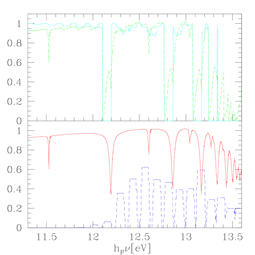
Figure 2: The three functions (in dimensionless units, relative to one) used to solve line radiative transfer in the H₂ Lyman-Werner bands and H i Lyman series. Top panel: first (solid line) and second (dashed-line) terms on the right hand side of equation (8). Bottom panel: the source term (solid line) and H₂ dissociation cross section $\sigma_{dis}$ (dashed line). The spectral resolution is $\Delta\nu/\nu=9.26\times 10^{-6}$ (i.e., 20,000 logarithmic bins in the energy range $11.2-13.6$ eV).

2.2 H₂ Chemistry and Cooling/Heating Processes

In Figure 3 we compare the chemical rates from the three compilations used most widely in cosmology. The labels on the top of each panel indicate the reaction and the name of the rate coefficient according to the author of the compilation: K (Shapiro & Kang, 1987), A (Abel et al., 1997) and H (Galli & Palla, 1998). The bottom-right panel compares the ro-vibrational H₂ cooling functions from Tegmark et al. (1997), Lepp & Shull (1983), and Galli & Palla (1998). We have assumed $x_{H_{2}}=10^{-3}$; for comparison we also show the Ly$\alpha$ cooling. The thin lines show additional cooling from the reactions k7, k9, k16, and k17 according to Shapiro & Kang (1987), assuming $x_{e}=0.5,x_{H_{2}^{+}}=10^{-7}$ and $x_{H^{-}}=10^{-7}$. These cooling processes are generally negligible. The cooling from reactions A8 and A10, $\Lambda_{H_{2}}=n_{H}(3.53k_{8}n_{H^{-}}+1.38k_{10}n_{H_{2}^{+}})$ eV cm^-3 s^-1 (Abel et al., 1997), can be important (horizontal dash-dotted line). The code can use each one of these rates, but in the following we will use the rates and H₂ cooling function from Galli & Palla (1998). We also include the additional cooling/heating processes from the aforementioned reactions. We neglect D and Li reactions and the formation of HeH⁺ molecules. They are negligible in the range of densities resolved by our simulations.

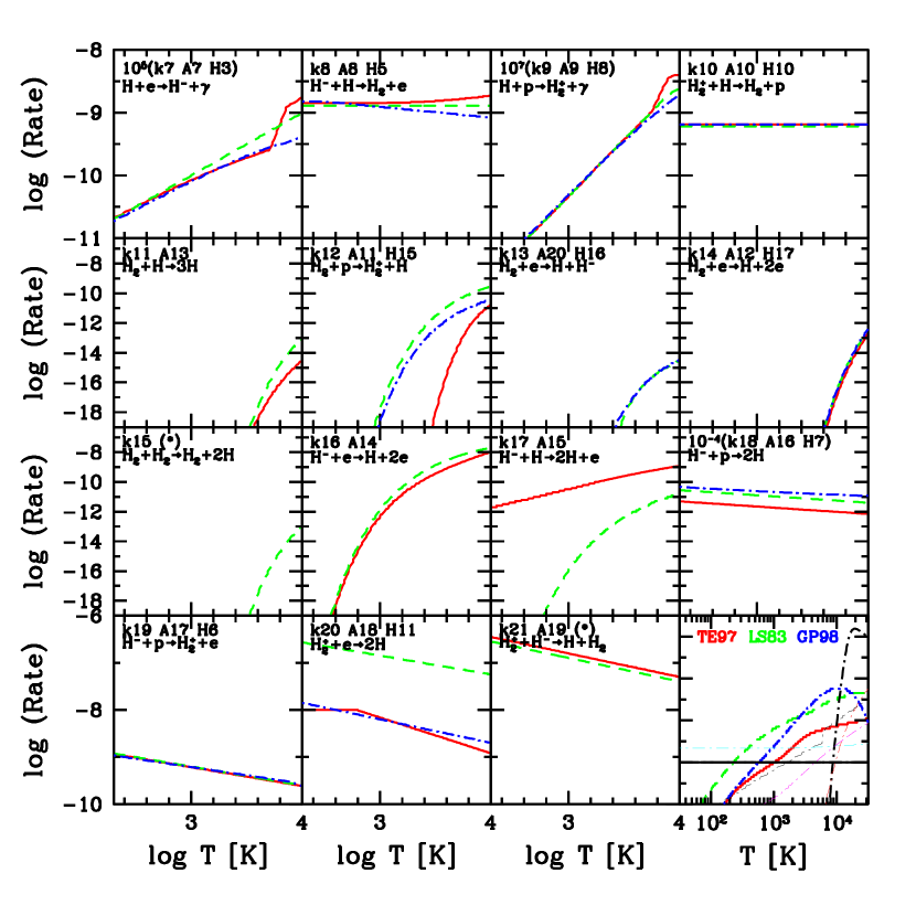
Figure 3: Comparison of rate compilations found in literature: Shapiro & Kang (1987) dashed lines, Galli & Palla (1998) dash-dotted lines, and Abel et al. (1997) solid lines. The bottom-right panel shows H₂ cooling functions from Tegmark et al. (1997) (solid line), Lepp & Shull (1983) (dashed line), and Galli & Palla (1998) (dot-dashed line). The thin lines in the same panel show cooling rates from the reactions, k7, k9, k16, k17 (Shapiro & Kang, 1987) and A8, A10 (Abel et al., 1997). In the simulations shown in this paper, we adopt the rates and the H₂ cooling function from Galli & Palla (1998). We also include cooling from the aforementioned reactions.

2.2.1 Heating by resonant scattering of Ly$\alpha$ photons

Generally, in scattering processes of photons with particles, the recoil of the particles causes the radiation field to exchange energy with the matter. In the case of resonance lines, contrary to electron scattering, the cumulative effects of atom recoils remain small even for large line optical depths. This happens because a photon in the red wing of a line is strongly biased to scatter back to the blue. Thus, the background intensity at the resonance line frequency develops only a slight asymmetry. The average relative shift in a Ly$\alpha$ photon energy, $E$, after having been scattered by a hydrogen atom at rest is $\langle\Delta E/E\rangle=-(h_{p}\nu/m_{H}c^{2})\approx-10^{-8}$, where $m_{H}$ is the mass of the hydrogen atom (Madau, Meiksin, & Rees, 1997) and $h_{p}$ is the Planck constant. If $T\ll h_{p}\nu_{\alpha}/k=1.2\times 10^{5}$ K, the energy is transferred from Ly$\alpha$ photon to the gas at a rate,

$${dE_{\alpha}\over dt}=-\left\langle{\Delta E\over E}\right\rangle h_{p}\nu_{\alpha}P_{\alpha},$$ (14)

where,

$$P_{\alpha}=\int d\Omega\int{J_{\nu}\over h_{p}\nu}\sigma_{\nu}^{Ly\alpha}d\nu,$$ (15)

is the Ly$\alpha$ scattering rate per H atom and $\sigma_{\nu}^{Ly\alpha}$ the Ly$\alpha$ absorption cross section.

The background at the Ly$\alpha$ frequency is produced mainly by redshifted non-ionizing UV photons (i.e., the photons emitted at the rest frame in the Lyman-Werner bands). All the other sources of Ly$\alpha$ photons have a negligible effect on heating of neutral IGM. For instance, compared to X-ray heating discussed in the next section, the heating produced by the scattering of Ly$\alpha$ photons emitted in the rest frame (not redshifted) from normal galaxies, is about 100 times less efficient (Madau et al., 1997).

2.2.2 Secondary Ionization and Heating from X-rays

Photoionization of H i , He i , and He ii by X-rays and EUV photons produces energetic photoelectrons that can excite and ionize atoms before their energy is thermalized. This effect can be important (Venkatesan, Giroux, & Shull, 2001) before reionization, when the gas is almost neutral and the spectrum of the background radiation is hard due to the large optical depth of the IGM to UV photons.

We provide analytic fits to the Monte Carlo results of Shull & van Steenberg (1985). Collisional ionization and excitation of He ii by primary electrons are neglected since, in a predominantly neutral medium, they are unimportant. The primary ionization rate for the species $i={\text{H\,\sc i}},{\text{He\,\sc i}},{\text{He\,\sc ii}}$ are,

$$\zeta^{i}=4\pi\int_{\nu_{i}}^{\infty}{J_{\nu}\over h_{p}\nu}\exp(-\tau_{\nu})\sigma_{\nu}^{i}d\nu,$$ (16)

where $\tau_{\nu}$ is the continuum optical depth, and $\sigma_{\nu}^{i}$ is the photoionization cross section of the species $i$. Secondary ionizations enhance the photoionization rates as follows:

$$\zeta_{s}^{{\text{H\,\sc i}}}=\zeta^{{\text{H\,\sc i}}}+\sum_{i={\text{H\,\sc i}},{\text{He\,\sc i}},{\text{He\,\sc ii}}}\zeta^{i}\langle\Phi^{{\text{H\,\sc i}}}(E_{0}^{i},x_{e})\rangle$$ (17)

$$\zeta_{s}^{{\text{He\,\sc i}}}=\zeta^{{\text{He\,\sc i}}}+\sum_{i={\text{H\,\sc i}},{\text{He\,\sc i}},{\text{He\,\sc ii}}}\zeta^{i}\langle\Phi^{{\text{He\,\sc i}}}(E_{0}^{i},x_{e})\rangle,$$ (18)

where $\langle\Phi^{{\text{H\,\sc i}}}(E_{0}^{i},x_{e})\rangle$ and $\langle\Phi^{{\text{He\,\sc i}}}(E_{0}^{i},x_{e})\rangle$ express the average number of secondary ionizations per primary electron of energy $E_{0}^{i}=h_{p}\nu-I^{i}$ weighted by the function $(J_{\nu}/h_{p}\nu)\exp(-\tau_{\nu})\sigma_{\nu}^{i}$. Here $I^{i}=h_{p}\nu_{i}$ is the ionization potential for the species $i$.

The photoionization heating rates for the species $i={\text{H\,\sc i}},{\text{He\,\sc i}}$ are given by,

$$\Gamma^{i}=4\pi\int_{\nu_{i}}^{\infty}{J_{\nu}\over h_{p}\nu}\exp(-\tau)\sigma_{\nu}^{i}E_{h}(E_{0}^{i},x_{e})d\nu.$$ (19)

In Appendix A we give analytic fits to the functions $\Phi^{{\text{H\,\sc i}}},\Phi^{{\text{He\,\sc i}}}$ and $E_{h}$. We express these functions in a form suited to minimize the computational time for the integrals in equations (17)–(19).

2.3 Sources spectrum and $\langle f_{esc}\rangle$

In Ricotti et al. (2001) we showed that the SED of a galaxy and $\langle f_{esc}\rangle$ are the main parameters that determine the relevance of positive feedback effects. In particular, we found that the Population III (metal-free) and mini-quasar (with spectral index $\alpha=1.8$) SED produce similar positive feedback regions (PFR). In this section, we explain how these ingredients are included in the code. We do not use the mini-quasar SED in our simulations. Apart from producing a stronger X-ray background, their effects should be analogous to those of the Population III SED.

Resolution elements that sink below the resolution limit of the simulation are allowed to form stars and therefore become sources of radiation according to the following equations:

$${d\rho_{*}\over dt} = \epsilon_{*}{\rho_{g}\over t_{*}},$$ (20)

$$S_{\nu} = {\epsilon_{UV}\over 4\pi}c^{3}{d\rho_{*}\over dt}g_{\nu}e^{-\tau_{\nu}}.$$ (21)

Star formation is implemented using the Schmidt law, where $\epsilon_{*}$ is the star formation efficiency, $\rho_{*}$ and $\rho_{g}$ are the stellar and gas density, respectively, and $t_{*}$ is the maximum of the dynamical time and cooling time. The parameter $\epsilon_{UV}$ is the ratio of energy density of the ionizing radiation field to the gas rest-mass energy density converted into stars, $g_{\nu}$ [photons Hz^-1] is the normalized SED,

$$\int_{\nu_{0}}^{\infty}g_{\nu}d\nu=1,$$

and $\tau_{\nu}$ is the internal opacity of the source. The escape fraction of ionizing photons, $\langle f_{esc}\rangle$, is defined as:

$$\langle f_{esc}\rangle=\int_{\nu_{0}}^{\infty}g_{\nu}e^{-\tau_{\nu}}d\nu,$$ (22)

where $\nu_{0}$ is the H i Lyc frequency. A value of $\langle f_{esc}\rangle$ $<1$ has the additional effect of producing harder source spectra because the gas optical depth is higher for UV and FUV photons than for X-ray photons. We include this effect modifying the SED using a frequency dependent optical depth

$$\tau_{\nu}=N_{{\text{H\,\sc i}}}(\sigma_{{\text{H\,\sc i}}}+a_{0}\sigma_{{\text{He\,\sc i}}}+a_{1}\sigma_{{\text{He\,\sc ii}}}).$$ (23)

Here, $a_{0}=N_{{\text{He\,\sc i}}}/N_{{\text{H\,\sc i}}}$ and $a_{1}=N_{{\text{He\,\sc ii}}}/N_{{\text{H\,\sc i}}}$ where $N_{i}$ is the column density of the species/ion $i$. The unknown parameters, $a_{0}$ and $a_{1}$, depend on the interstellar medium (ISM) properties of the galaxies, including clumping. Based on the results of simple 1D radiative transfer simulations presented in Ricotti et al. (2001), we chose $a_{0}=0.01$ and $a_{1}=10$ when we use the Population III SED, and $a_{0}=0.1$ and $a_{1}=10$ when we use the Population II SED. These values are calculated placing the source of radiation in the center of a spherical galaxy with a gas density profile calculated with high-resolution numerical simulations (Abel, Bryan, & Norman, 2000). We did not consider the effects of a clumpy ISM. Given the value of $\langle f_{esc}\rangle$, $N_{{\text{H\,\sc i}}}$ is calculated from equations (22)–(23) using a bisection algorithm.

The spatial resolution of the code is determined by the dimensionless SLH parameter, $B_{*}$. The code switches from Lagrangian to Eulerian when the deformation of the spatial grid exceeds a critical value that is approximatively $1/B_{*}$ the undeformed cell size. Therefore, the comoving spatial resolution is about $L_{box}/(N_{box}B_{*})$, where $L_{box}$ is the box size and $N_{box}^{3}$ is the number of cells in the box. Usually we use $B_{*}=10$ for $N_{box}=64$ ($262,144$ cells), $B_{*}=16$ for $N_{box}=128$ (2 million cells) and $B_{*}=25$ for $N_{box}=256$ (17 million cells). The gravity force is calculated by a P³M algorithm with the Plummer softening parameter equal to $1/2B_{*}$. This ensures that the gravity force is accurate on our resolution scale, and thus $1/B_{*}$ is a real rather than nominal resolution. The nominal resolution is twice higher.

We allow the spectral energy distribution, $g_{\nu}$, to be chosen from the following:
i) Population II: metallicity $Z=0.04$ Z_⊙, evolutionary tracks evolved to $t=1$ Gyr, continuous SF law, Salpeter IMF with star masses between $1<M_{*}<100$ M_⊙ (Leitherer et al., 1995). Wolf-Rayet stars are responsible for the substantial EUV emission in this SED.
ii) Population III : metallicity $Z=0$, non-evolved, instantaneous SF law, Salpeter IMF with star masses between $1<M_{*}<100$ M_⊙ (Tumlinson & Shull, 2000). Note the importance of He ii ionizing radiation in this SED.
iii) Population III : metallicity $Z=0$, evolutionary tracks evolved to $t=1$ Gyr, continuous SF law, Salpeter IMF with star masses between $1<M_{*}<100$ M_⊙ (Brocato et al., 1999, 2000). This SED calculation differs substantially from (ii) since it does not include He ii ionizing photons.
In Figure 4 we show the analytical fits implemented in the code for these three SEDs. In our simulations we will use only the non-evolved Population III SED (ii) and the Population II SED (i). The evolved Population III SED (iii) is implemented in the code but never used. We show it just for comparison since calculations from different authors of the Population III SEDs are still in disagreement.

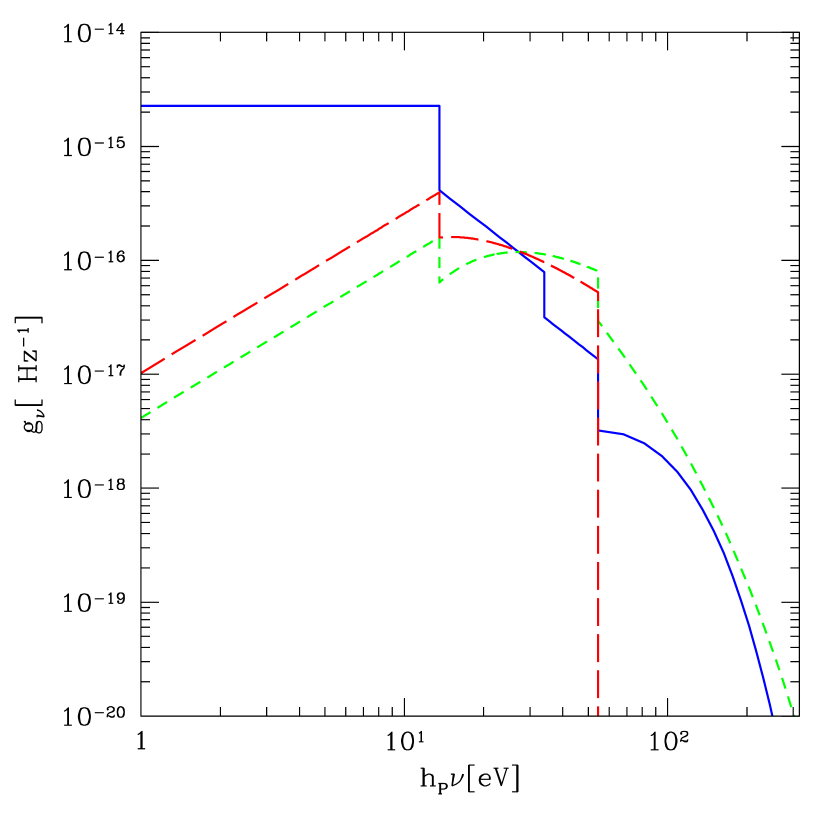
Figure 4: Analytical fits to the normalized Population II SED for a continuous SF law evolved to $t=1$ Gyr (solid line), non-evolved Population III SED for an instantaneous SF law (short-dashed line) and Population III SED for a continuous SF law evolved to $t=1$ Gyr (long-dashed line). See text for further explanation.

The free parameter $\epsilon_{UV}$ is the ratio of energy density of the ionizing radiation field to the gas rest-mass energy density converted into stars ($\rho_{*}c^{2}$). Thus, $\epsilon_{UV}=(\overline{h_{p}\nu}/m_{H}c^{2})\epsilon_{UV}^{*}$, where $\epsilon_{UV}^{*}$ is the number of ionizing photons per baryon converted into stars. The value of $\epsilon_{UV}$ depends on the IMF and the metallicity of the stellar population. Assuming a Salpeter IMF with star masses between $1~{}{\rm M}_{\odot}\leq{\rm M}^{*}\leq 100~{}{\rm M}_{\odot}$, we have $(\epsilon_{UV}/4\pi)=1.1\times 10^{-5}$, $\overline{h_{p}\nu}/(13.6~{}{\rm eV})=1.76$ for the Population II SED and $(\epsilon_{UV}/4\pi)=2.5\times 10^{-5}$, $\overline{h_{p}\nu}/(13.6~{}{\rm eV})=2.47$ for the (ii) Population III SED. Theoretical works (Uehara et al., 1996; Larson, 1998; Nakamura & Umemura, 1999, 2001) have shown that the IMF of metal-free stars could be dominated by massive stars or might have a bimodal IMF (lacking in intermediate mass stars). If the IMF is dominated by very massive stars ($M\sim 300$ M_⊙) that eventually evolve into black holes (Bromm, Kudritzki, & Loeb, 2001), it is possible to have $(\epsilon_{UV}/4\pi)\gg 2.5\times 10^{-5}$.

The free parameter $\langle f_{esc}\rangle$ is the fraction of ionizing photons escaping from the resolution element of the simulation. According to its definition, this parameter is, in general, resolution and time dependent. Theoretical studies (Ricotti & Shull, 2000; Wood & Loeb, 2000) have shown that $\langle f_{esc}\rangle$, defined as the fraction of ionizing photons escaping from a galaxy halo, decreases at increasing redshift and increasing mass of the halos (assuming constant star formation efficiency). In particular, Ricotti & Shull (2000) provide analytic formulae for $\langle f_{esc}\rangle$ $(z_{vir},\epsilon,f_{g},M_{DM})$ as a function of the star formation efficiency (SFE), $\epsilon$, normalized to the Milky Way value, the redshift of virialization, $z_{vir}$, the DM halo mass, $M_{DM}$, and the fraction of collapsed gas $f_{g}$. The following formula, for example,

$$\langle f_{esc}\rangle={4.44\over(\epsilon f_{g})^{1/3}}\left({10^{6}~{}{\rm M}_{\odot}\over M_{DM}}\right)^{1\over 3}\exp\left[-0.94(1+\log f_{g}^{2\over 3}){z_{vir}+1\over\epsilon^{1/3}}\right],$$ (24)

is valid for “small-halo” objects ($M_{DM}\leq 10^{8}M_{\odot}[(1+z_{vir})/10]^{-1.5}$), a constant SFE $4<\epsilon<400$ (i.e., the ionizing flux is proportional to the gas mass of the halo) and assuming a power law for the ionizing photon luminosity function of the OB associations with slope $\alpha=2$ (Dove & Shull, 1994; Kennicutt, Edgar, & Hodge, 1989), lower limit $S_{1}=10^{48}$ photons s^-1, and no upper limit. Equation (24) cannot be used in the code, because the definition of $\langle f_{esc}\rangle$ depends on the spatial resolution of the simulation. Instead, $\langle f_{esc}\rangle$ in equation (24) is a function of the halo mass. Nevertheless, even if $\langle f_{esc}\rangle$ in the code is larger than $\langle f_{esc}\rangle$ in equation (24), depending on the spatial resolution of the code, the functional dependence of $\langle f_{esc}\rangle$ on the virialization redshift should be robust. In this study, we will consider $\langle f_{esc}\rangle$ as a constant free parameter. Equation (24) is simply used to provide a first-order estimate of reasonable values for $\langle f_{esc}\rangle$ at high redshift. We plan to relax this assumption in future work.

3 Resolution Studies

In this section we investigate the numerical convergence of our simulations. Simulating the formation of the first galaxies is computationally challenging. It requires high mass resolution in order to resolve the internal structure of each low-mass object with a sufficient number of dark matter particles and grid cells. Moreover, since the first objects arise from the collapse of the most massive and rare density perturbations at redshift $z\sim 30$, we need a sufficiently large box to include at least a few 3 $\sigma$ perturbations of the initial density field. These requirements translate into the need for simulations with large mass dynamical range (i.e., a large number of cells and DM particles in the box). We have been able to run a few simulations with the maximum feasible resolution of $256^{3}$ cells, but the bulk of the study consists of runs with $128^{3}$, and $64^{3}$ cells.

In Table 1 we list the runs used to test the convergence of the simulation. In all these test runs (but one: 256L1p3) the radiative transfer algorithm has been shut down. Therefore, the stars were able to form but did not produce any feedback effects.

Table 1: List of simulations.

RUN	$N_{box}$	$L_{box}$	Mass Resolution	$B_{*}$	$\left({\epsilon_{UV}\over 4\pi}\right)$$\langle f_{esc}\rangle$	$\epsilon_{*}$
		($h^{-1}$ Mpc)	($h^{-1}$ M⊙)
64L05B8	64	0.5	$3.94\times 10^{4}$	8	0	0.2
64L05	64	0.5	$3.94\times 10^{4}$	10	0	0.2
64L05B12	64	0.5	$3.94\times 10^{4}$	12	0	0.2
64L05B16	64	0.5	$3.94\times 10^{4}$	16	0	0.2
64L1	64	1.0	$3.15\times 10^{5}$	10	0	0.2
64L1B16	64	1.0	$3.15\times 10^{5}$	16	0	0.2
128L05	128	0.5	$4.93\times 10^{3}$	10	0	0.2
128L1	128	1.0	$3.94\times 10^{4}$	10	0	0.2
128L1B16	128	1.0	$3.94\times 10^{4}$	16	0	0.2
256L1	256	1.0	$4.93\times 10^{3}$	10	0	0.2
256L2	256	2.0	$3.94\times 10^{4}$	10	0	0.2
256L1p3	256	1.0	$4.93\times 10^{3}$	25	$2.5\times 10^{-6}$	0.1

Note. — Parameter description. Numerical parameters: $N_{box}^{3}$ is the number of grid cells, $L_{box}$ is the box size in comoving $h^{-1}$ Mpc, $B_{*}$ is a parameter that regulates the maximum deformation of the Lagrangian mesh: the spatial resolution is $\sim L_{box}/(N_{box}B_{*})$. Physical parameters: $g_{\nu}$ is the normalized SED, $\epsilon_{*}$ is the star formation efficiency, $\epsilon_{UV}$ is the ratio of energy density of the ionizing radiation field to the gas rest-mass energy density converted into stars (depends on the IMF), and $\langle f_{esc}\rangle$ is the escape fraction of ionizing photons from the resolution element.

3.1 Mass resolution and Box Size

We check the convergence of the simulations with two sets of runs. The first set that includes runs 64L1, 128L1, and 256L1 has a constant box size $L_{box}=1$ $h^{-1}$ Mpc, and mass resolutions $M_{DM}=3.15\times 10^{5},3.94\times 10^{4}$, and $4.93\times 10^{3}$ $h^{-1}$ M_⊙, respectively. The second set that includes runs 64L05, 128L1, and 256L2 has a constant mass resolution $M_{DM}=3.94\times 10^{4}$ $h^{-1}$ M_⊙ and box sizes $L_{box}=0.5,1$, and 2 $h^{-1}$ Mpc, respectively. If we assume that a physical output of the simulation, $C$, scales with $N_{box}$ as

$$C=C_{\infty}+{\Delta\over(N_{box})^{\alpha}}$$ (25)

(a usual assumption in convergence analysis of numerical simulations), we can determine the asymptotic limit $C_{\infty}=\lim_{N_{box}\rightarrow\infty}C$ if we have three simulations that differ only in the value of $N_{box}$. Since the choice of equation (25) is somewhat arbitrary, the estimate of the convergence of the simulations is perhaps not rigorous and the results should be interpreted simply as a sign of convergence. We never used resolution studies to correct the results our the simulations for resolution or box size effects.

The curves in Figure 5 show equation (25) as a function of $N_{box}$, where the observable $C$ is the redshift $z$ at which the star fraction is $\log f_{star}=\log(\rho_{star}/\rho_{b})={\rm const.}$ In Figure 5 (left) the data points are for the first set of simulations; therefore, the asymptotic limits $C_{\infty}$ (horizontal lines) show the redshifts at which $\log f_{star}=-6,-5,-4,-3,-2.2$ for a simulation with infinite mass resolution and $L_{box}=1$. Figure 5 (right) is analogous to Figure 5 (left) but for the second set of simulations. Here, the asymptotic limits $C_{\infty}$ show the redshifts at which $\log f_{star}=-6,-5,-4,-3.5$ for a simulation with infinite box size and mass resolution $M_{DM}=3.94\times 10^{4}$ $h^{-1}$ M_⊙.

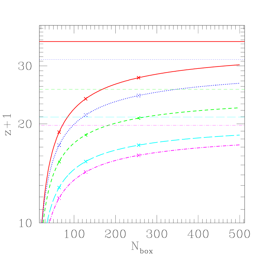
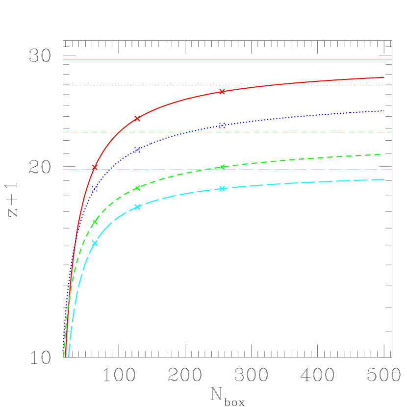
Figure 5: Resolution studies. (Left) we use a set of three simulations (256L1, 128L1, and 64L1) with different mass resolution and $L_{box}=1$ $h^{-1}$ Mpc, to extrapolate to the infinite resolution limit (thin horizontal lines). The curves, from top to bottom, show $z+1$ as a function of $N_{box}$ [eq. (25)] at constant $\log f_{stars}=-6,-5,-4,-3,-2.2$, and crosses on each curve show the three data points. (Right) same as left but for a set of three simulations (256L2, 128L1, and 64L05) with different box sizes and the same mass resolution. The thin horizontal lines show the infinite box size limits. The lines from top to bottom are at constant $\log f_{stars}=-6,-5,-4,-3.5$.

In Figure 6 we summarize the mass resolution and box-size convergence studies. The curves show the fraction of baryons in stars, $f_{star}$, for the two sets of simulations discussed in the previous paragraph. The triangles show $f_{star}$ in the limit of a simulation with infinite mass resolution and $L_{box}=1$ $h^{-1}$ Mpc. The squares show $f_{star}$ for a simulation with infinite box size and mass resolution $M_{DM}=3.94\times 10^{4}$ $h^{-1}$ M_⊙. Figure 6 shows that the 256L1 run is the closest to the convergence limit.

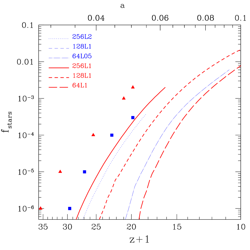
Figure 6: Fraction of baryons in stars versus redshift for two sets of simulations with different resolution and box sizes. The three thick lines show 256L1, 128L1, and 64L1 simulations with constant box size ($L_{box}=1$ $h^{-1}$ Mpc), and varying mass resolutions ($M_{DM}=3.15\times 10^{5},3.94\times 10^{4}$, and $4.93\times 10^{3}$ $h^{-1}$ M_⊙, respectively). The triangles show $f_{star}$ as a function of redshift in the limit of a simulation with infinite mass resolution and $L_{box}=1$ $h^{-1}$ Mpc. The three thin lines show 64L05, 128L1, and 256L2 simulations, with constant mass resolution ($M_{DM}=3.94\times 10^{4}$ $h^{-1}$ M_⊙) and varying box sizes ($L_{box}=0.5,1$, and 2 $h^{-1}$ Mpc, respectively). The squares show $f_{star}$ as a function of redshift in the limit of infinite box size and mass resolution $M_{DM}=3.94\times 10^{4}$ $h^{-1}$ M_⊙. Note that the simulation 128L1 appears in both sets; therefore there are only five lines in the plot.

The level of convergence of a simulation can be easily understood from the plot in Figure 7. The cusp-shaped curves show the fraction of cooled gas in collapsed objects at $z+1=35,30,25,20,15,10,4$ (from bottom to top) calculated with the Press-Schechter formalism. The gas collapsed in the DM halo is assumed to be shock-heated to about its virial temperature. In order to form stars, the gas cooling time $t_{cool}(z)$ must be shorter than the Hubble time $1/H(z)$. We roughly estimate the fraction of baryons able to cool and form stars by multiplying the virialized object fraction by the cooling efficiency $\epsilon_{cool}=max[1/t_{cool}(z)H(z),1]$. Note that $\epsilon_{cool}<1$ for masses typical of both “small-halo” objects and galaxy clusters. The comoving size of the box determines the DM mass of the most massive halo in the simulation, and the mass resolution determines the mass of the least massive object resolved. The oblique lines show the DM mass of the most massive halo in simulations of box sizes $L_{box}=0.5,1,2$ $h^{-1}$ Mpc (from top to bottom). The vertical lines show the mass of the least massive DM halo for which we resolve the SF in simulations with mass resolution $M_{DM}=4.93\times 10^{3},3.94\times 10^{4}$, and $3.15\times 10^{5}$ $h^{-1}$ M_⊙ (from left to right). As a quick reference, the vertical lines correspond to $256^{3},128^{3},64^{3}$ cubes with $L_{box}=1$ $h^{-1}$ Mpc. These minimum masses are about 100 times the mass resolution of the simulation. That means that we need to resolve each halo with about 100 cells.

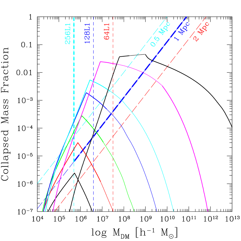
Figure 7: Fraction of collapsed gas as a function of DM halo mass at $z+1=35,30,25,20,15,10,4$ (from bottom to top). We use the Press-Schechter formalism and a simple estimate for the fraction of collapsed gas based on the cooling time (see text). The thin portions of the curves correspond to virial temperatures $10^{4}\lower 2.15277pt\hbox{$\;\buildrel<\over{\sim}\;$}T_{vir}\lower 2.15277pt\hbox{$\;\buildrel<\over{\sim}\;$}10^{5}$ K. In these halos, the cooling is very efficient and all the gas is collapsed; the thick portions of the curves on the left are “small-halo” objects ($T_{vir}<10^{4}$ K) and on the right objects with $T_{vir}>10^{5}$ K. The vertical lines correspond to the smallest halo mass fully resolved by simulations with mass resolution $M_{DM}=4.93\times 10^{3},3.94\times 10^{4}$, and $3.15\times 10^{5}$ $h^{-1}$ M_⊙ (from left to right). As a quick reference they correspond to $256^{3},128^{3},64^{3}$ cubes with $L_{box}=1$ $h^{-1}$ Mpc. The oblique lines show the largest halo mass that we can find in cubes with $L_{box}=0.5,1,2$ $h^{-1}$ Mpc. For example, the two thicker vertical and oblique lines delimit the galaxies fully resolved in the 256L1 simulation.

Given the box size and the mass resolution of the simulation, the point of intersection of the appropriate vertical and oblique lines shows the redshift of formation and the mass of the first object in the simulation. For example, the two thicker vertical and oblique lines delimit the masses resolved in the $256^{3}$ cells, $L_{box}=1$ $h^{-1}$ Mpc simulation. In this simulation, the first objects have masses $M\sim 5\times 10^{5}$ $h^{-1}$ M_⊙ and form between $z=29$ and $z=34$. Moreover, this simulation can resolve the bulk of the collapsed baryons up to redshift $z\sim 5$.

In this study we show both integrated physical quantities such as SFR, background radiation intensity, chemical abundances, and also the properties of individual bound objects formed in the simulations. We identify bound objects with the DENMAX algorithm (Bertschinger & Gelb, 1991). The results of DENMAX depend on the choice of the free parameter, $G=L_{box}/L_{G}$, which defines the smoothing length, $L_{G}$, of the particle density field. In Appendix B we show how to select the smoothing parameter when comparing simulations with different resolution/box sizes.

In Figure 8 we compare the SFR at $z=15$ as a function of halo mass for simulations with different resolutions and box sizes. The halos have been identified using DENMAX with smoothing parameter $G=400$ for the 128 boxes and $G=1000$ for the 256 box. It is evident that the 128L1 run does not sufficiently resolve small mass ($M_{DM}\leq 2\times 10^{7}$ $h^{-1}$ M_⊙) halos, and the 128L0.5 run does not have enough large mass objects.

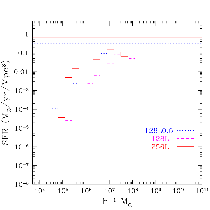
Figure 8: Global SFR at $z=15$ as a function of DM halo mass. The three histograms show the same simulation at different resolutions and box sizes. The solid line shows the simulation with $256^{3}$ cells and $L_{box}=1$ $h^{-1}$ Mpc, the dashed-line $128^{3}$, $L_{box}=1$ $h^{-1}$ Mpc, and the dotted line $128^{3}$, $L_{box}=0.5$ $h^{-1}$ Mpc. The halos have been identified using DENMAX with smoothing parameter $G=400$ for the $128^{3}$ boxes and $G=1000$ for the $256^{3}$ box. The three horizontal lines above the histograms show the total (integrated over all masses) SFR for the same simulations.

The minimum redshift to which we can evolve the simulations depends on the box size. For 2, 1, and 0.5 $h^{-1}$ Mpc boxes, we can evolve the simulation until redshifts $z\approx 6,9$, and 12 respectively. Thereafter, scales of the order of the box size become nonlinear, and the box ceases to be a representative sample of the universe.

3.2 Spatial resolution

The spatial resolution of the grid is regulated by the softening parameter $B_{*}$, which sets the maximum deformation of the grid (the cell size can only become $\sim 2B_{*}$ times smaller than the initial value). The value of $B_{*}$ cannot be arbitrarily large because the grid has a “numerical tension” that prevents excessive deformation.

In Figure 9 we show the fraction of baryons in stars, $f_{star}$, as a function of redshift for values of $B_{*}=8,10,12,16$. It appears that the results are not sensitive to the value of $B_{*}$, at least in the explored range. The only noticeable effect is a slight delay in the formation of the first objects as $B_{*}$ increases.

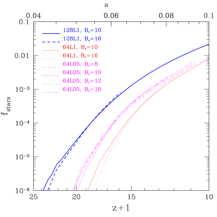
Figure 9: Fraction of baryons in stars versus redshift for simulations with different values of the spatial resolution parameter, $B_{*}$. The two thick lines have $N_{box}=128$, $L_{box}=1$ $h^{-1}$ Mpc ($B_{*}=10,16$). The thin solid and dotted lines have $N_{box}=64$, $L_{box}=1$ $h^{-1}$ Mpc ($B_{*}=10,16$). The other thin lines have $N_{box}=64$, $L_{box}=0.5$ $h^{-1}$ Mpc ($B_{*}=8,10,12,16$). The spatial resolution is about $L_{box}/(N_{box}B_{*})$.

4 Discussion and Summary

We have introduced a 3D cosmological code with radiative transfer suited to simulate the formation of the first objects self-consistently. We use the “Softened Lagrangian Hydrodynamics” (SLH-P³M) code (Gnedin, 1995, 1996; Gnedin & Bertschinger, 1996; Gnedin & Abel, 2001) to solve the system of time-dependent equations of motion for dark matter particles (P³M algorithm), gas particles (quasi-Lagrangian deformable mesh using the SLH algorithm), and “stellar-particles” formed using the Schmidt law in resolution elements that sink below the numerical resolution of the code. The highest mass resolution that we achieve is $M_{DM}=4.93\times 10^{3}$ $h^{-1}$ M_⊙, and the highest spatial resolution is $156$ $h^{-1}$ pc comoving. We solve the continuum radiative transfer with the OTVET approximation (Gnedin & Abel, 2001), and we solve exactly the line radiative transfer in the H₂ Lyman-Werner bands of the background radiation. Detailed atomic and molecular physics is included, although we have not included “supernova feedback” (work in progress).

Including ionization from secondary electrons in the simulation does not produce significant changes of the IGM temperature or ionization of H and He. Secondary electrons are important when the ionizing spectrum is hard and UV photons do not dominate the ionization rate. X-rays (keV energies) in the background radiation are produced either by Wolf-Rayet stars in Population II or by the much hotter Population III stars. Nevertheless, the ionizing radiation background is dominated by the UV photons in the spectral features produced by the redshifted resonant He i and He ii Ly$\alpha$ lines. In Figure 10 we show three examples of background (i.e., spatially averaged) radiation spectra: for a Population III SED and $\langle f_{esc}\rangle$ $=1$, for a Population III SED and $\langle f_{esc}\rangle$ $=10^{-2}$, and for a Population II SED and $\langle f_{esc}\rangle$ $=10^{-2}$. The spectrum is rather complex, but we can identify spectral features associated with the redshifted resonant H i , He i , and He ii Ly$\alpha$ lines, and the jumps at the H i , He i , and He ii ionization thresholds. In the spectral region between 11.2 - 13.6 eV, responsible for the photodissociation of H₂, we solve the line radiative transfer using a grid with $20,000$ frequency bins. An enlarged figure of this spectral region would show more clearly the fine absorption features associated with H₂ and resonant H i line opacity in the IGM. For the rest of the spectrum radiative transfer is solved for both the background and the spatially varying radiation dividing the spectrum in 4 frequency intervals [(i) optically thin between 1 - 11.2 eV, (ii) H i ionizing radiation, (iii) He i ionizing radiation and (iv) He ii ionizing radiation] resolved with 300 logarithmic bins altogether.

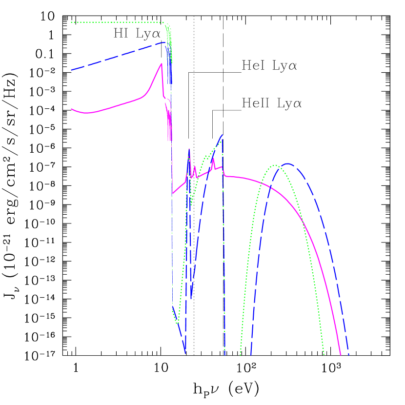
Figure 10: Spectrum of the background radiation, $J_{\nu}$. We show three representative examples: (i) using a Population III SED with $\langle f_{esc}\rangle$ $=1$ (solid line); (ii) using a Population III SED with $\langle f_{esc}\rangle$ $=10^{-2}$ (dashed line); (iii) using a Population II SED with $\langle f_{esc}\rangle$ $=10^{-2}$ (dotted line). The dotted vertical line shows the He i ionization frequency, and the dashed vertical line shows the He ii ionization frequency.

In Figure 11 we show an example of 3D rendering of H ii regions at $z=27.6$ from one of our simulations ($N_{box}=128$, $L_{box}=1$ $h^{-1}$ Mpc) with radiative transfer. The small H ii regions produced by “small-halo” objects (the first “large-halo” objects form much later, cooling by H i Ly$\alpha$, at $z\lower 2.15277pt\hbox{$\;\buildrel<\over{\sim}\;$}18$) are clustered along the dense filaments of the cosmic large scale structure. In Figure 12 we show the global SFR as a function of redshift in the 256L1p3 run (thick solid line) compared to the same simulation without radiative feedback effects (thin solid line) and to a case where we do not allow the formation of any “small-halo” objects (thin dashed line). It is evident that the bursting mode of SF appears in the simulation with radiative feedback. The formation of “small-halo” objects is not dramatically suppressed by radiative feedback effects. In Paper II we study the nature of the feedback mechanism and the dependence of the SFR on the free parameters ($\langle f_{esc}\rangle$, $\epsilon_{*}$, $\epsilon_{UV}$, and $g_{\nu}$) related to the unknown sub-grid physics (stellar IMF, star formation efficiency, and ISM properties at high-redshift).

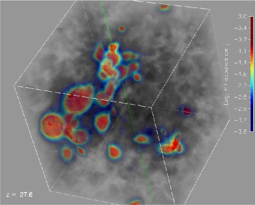
Figure 11: Example of 3D rendering of H ii regions at $z=27.6$. The colors code the logarithm of H ii abundance. “small-halo” objects produce small H ii regions clustered along the large scale structure filaments.

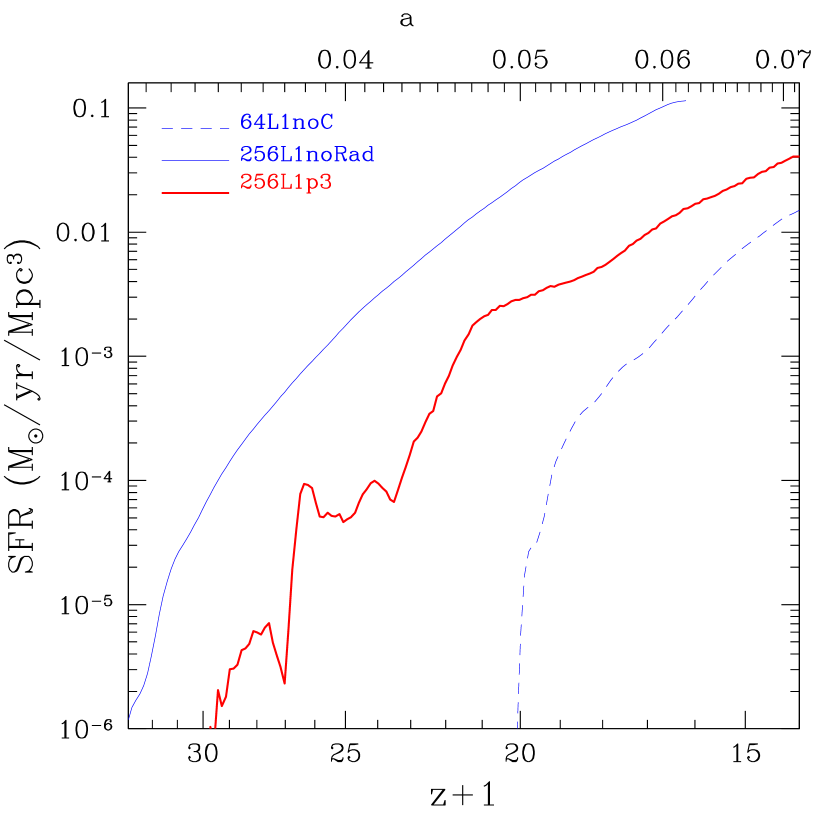
Figure 12: Global SFR versus redshift. The thick solid line shows the 256L1p3 run ($N_{box}=256$, $L_{box}=1$ $h^{-1}$ Mpc, Population III SED, $\langle f_{esc}\rangle$ $=0.1$, $\epsilon_{*}=0.1$, and $(\epsilon_{UV}/4\pi)=2.5\times 10^{-5}$) that includes continuum and line radiative transfer and all the physics discussed in this paper. As a comparison, we show the same simulation without radiative transfer (thin solid line) and a simulation ($N_{box}=64$, $L_{box}=1$ $h^{-1}$ Mpc) that forms only “large-halo” objects since we did not include H₂ cooling and radiative transfer (thin dashed line).

Two important processes are not yet included in the simulations: H₂ self-shielding and feedback from SN explosions. In some of our simulations with radiative transfer, we find that H₂ in the filaments has a column density $N_{H_{2}}\geq 10^{15}$ cm^-2, sufficient to shield the outgoing radiation emitted by embedded sources and the ingoing radiation emitted by external sources. We could crudely include the effect of H₂ self-shielding for the outgoing radiation emitted by each source embedded in the filaments, modifying the source spectrum in the Lyman-Werner bands according to the 1D radiative transfer calculations shown in Figure 5 in Ricotti et al. (2001). A complete treatment of line radiative transfer would necessarily require some approximation, since it is impossible to achieve the frequency resolution needed for the exact calculation. We have decided not to implement any of these two possibilities, based on the first results of the simulations. In Paper II we will show that the SF is not suppressed by the dissociating radiation, even if we neglect H₂ self-shielding. The inclusion of self-shielding will not affect the global SFR in a significant way, since the primary feedback process that regulates the star formation is not H₂ photodissociation.

Supernova explosions could be important sources of feedback, both of heat and ionization. They could also produce a self-regulating global star formation and contribute to the transport of metals in the low density IGM. Unfortunately, we do not yet understand the correct modeling of their dynamical and thermal effects on the ISM/IGM. An approximate treatment of SN mechanical and thermal energy input is currently implemented in the code. We did not use this feature of the code, because we prefer to study the effects of radiative feedback and mechanical feedback from SN explosions separately. Moreover, we are not confident that the treatment of SN explosions in the code is appropriate, given the complexity of ISM in galaxies. The investigation of the effects of mechanical feedback from SNe explosions will be the subject of our future work.

Appendix A Secondary Ionization and Heating from X-rays

For photoelectron energies $E_{0}^{i}\gg 100$ eV we use the fits given by Shull & van Steenberg (1985). For lower energy photoelectrons we have made fits to the Monte Carlo results shown in Figure 3 of the aforementioned paper. The functional form of the fits allow us to integrate in photon frequency, factoring out the dependency on $x_{e}$. We pre-calculate the integrals and store the results in three-dimensional tables for each frequency bin in order to avoid computationally intensive calculations.

The fraction of secondary ionizations per primary electron of energy $E_{0}^{i}$ is $\Phi^{j}(E_{0}^{i},x_{e})$, where $E_{0}^{i}=h_{p}\nu-I^{i}$ with $I^{i}$ ground-state ionization potential of the species $i$ and

$$\Phi^{j}(E_{0}^{i},x_{e})=\left(E_{0}^{i}\over I^{j}\right)[y_{1}(j)f_{1}(E_{0}^{i})-y_{2}(j)f_{2}(E_{0}^{i})],$$ (A1)

where

$$f_{1}=\begin{cases}0&\text{if $E_{0}^{i}<28$ eV}\\ 1&\text{if $E_{0}^{i}\geq 28$ eV}\\ \end{cases}~{}~{}~{}f_{2}=\begin{cases}0&\text{if $E_{0}^{i}<28$ eV}\\ (28~{}{\rm eV}/E_{0}^{i})^{0.4}&\text{if $E_{0}^{i}\geq 28$ eV}.\\ \end{cases}$$ (A2)

Here, since we neglect ionization and excitation of He ii from energetic primary electrons, $i={\text{H\,\sc i}},{\text{He\,\sc i}},{\text{He\,\sc ii}}$ and $j={\text{H\,\sc i}},{\text{He\,\sc i}}$. Since a fraction of the energy of primary photoelectrons goes to secondary ionizations, the heating rates from H i and He i photoionizations are less efficient by the complementary factor,

$$E_{h}(E_{0}^{i},x_{e})=E_{0}^{i}[1-y_{1}(heat)f_{1}(heat)+y_{2}(heat)f_{2}(heat)],$$ (A3)

where

$$f_{1}=\begin{cases}0&\text{if $E_{0}^{i}<11$ eV}\\ 1&\text{if $E_{0}^{i}\geq 11$ eV}\\ \end{cases}~{}~{}~{}f_{2}=\begin{cases}0&\text{if $E_{0}^{i}<11$ eV}\\ (11~{}{\rm eV}/E_{0}^{i})^{0.7}&\text{if $E_{0}^{i}\geq 11$ eV}.\\ \end{cases}$$ (A4)

The high energy limits of equations (A1)–(A3) are the functions $y_{1}$ that are given by Shull & van Steenberg (1985), and $y_{2}$ has the form,

$$y_{1} = C(1-x_{e}^{b})^{c}$$ (A5)

$$y_{2} = Cx^{a}(1-x_{e}^{b})^{c},$$ (A6)

with $0\leq x_{e}\leq 1$. The coefficients for equation (A6) are listed in Table 2 and the fits are shown in Figure 13.

Table 2: Fitting Coefficients.

Parameter	$C$	$a$	$b$	$c$
$y_{1}({\text{H\,\sc i}})$	0.3908	–	0.4092	1.7592
$y_{1}({\text{He\,\sc i}})$	0.0554	–	0.4614	1.6660
$y_{1}(heat)$	1.0	–	0.2663	1.3163
$y_{2}({\text{H\,\sc i}})$	0.6941	0.2	0.38	2.0
$y_{2}({\text{He\,\sc i}})$	0.0984	0.2	0.38	2.0
$y_{2}(heat)$	3.9811	0.4	0.34	2.0

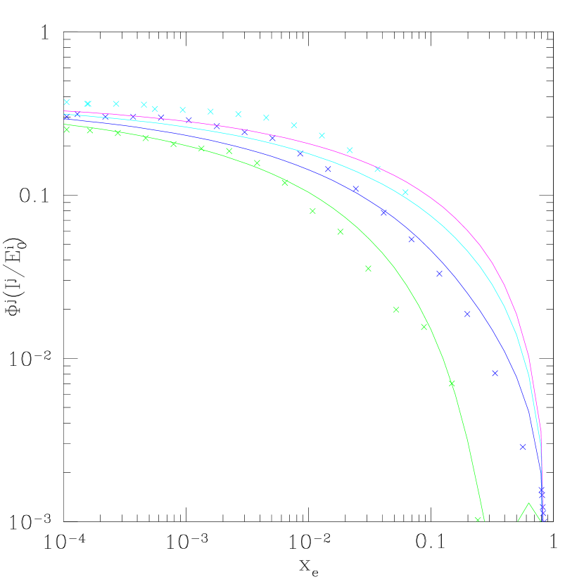
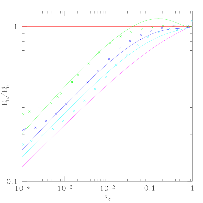
Figure 13: (Left) Fraction of energy deposited as H i ionization per primary electron of energy $E_{0}^{i}$, as a function of the electron fraction $x_{e}$. The data points and curves are for $E_{0}^{i}=28,50,100,200$ eV from bottom to top. (Right) Fraction of energy deposited as heat per primary electron of energy $E_{0}^{i}$, as a function of $x_{e}$. The data points and curves are for $E_{0}^{i}=2,11,28,50,200$ eV from top to bottom.

Appendix B Group-finding Algorithm

The DENMAX algorithm (Bertschinger & Gelb, 1991) identifies halos as maxima of the smoothed density field. The algorithm assigns each particle in the simulation to a group (halo) by moving each particle along the gradient of the density field until it reaches a local maximum. Unbound particles are then removed from the group.

The results of DENMAX depend on the degree of smoothing used to define the density field. A finer resolution in the density field will split large groups into smaller subunits and vice versa. This arbitrariness in results is a common problem of any group-finding algorithm, and it is not only a numerical problem but often a real physical ambiguity. Especially at high redshift, since the merger rate is high, it is difficult to identify or define a single galaxy halo.

Here we compare the mass function obtained using DENMAX with different smoothing scales $L_{G}=L_{box}/G$ with the Press-Schechter formalism. The main aim is to choose the parameter $G$ consistently in order to compare the results from simulations with an arbitrary number of cells in the box $N_{box}^{3}$. The mass of a DM particle is $M_{p}=8.26\times 10^{10}[(L_{box}/1h^{-1}{\rm Mpc})^{3}/N_{box}^{3}(\Omega_{m}/0.3)]$ $h^{-1}$ M_⊙ and the comoving space resolution $L_{res}=L_{box}/(B_{*}N_{box})$.

If we impose that each group has a minimum of $N_{p}$ DM particles, we have $L_{G}\geq N_{p}^{1/3}L_{res}$, which implies,

$$G\leq{B_{*}N_{box}\over N_{p}^{1/3}}<{B_{*}N_{box}},$$ (B1)

where $B_{*}$ is the resolution parameter. The inequality on the right-hand side is obtained by imposing $N_{p}\geq 1$. Another constraint on $G$ can be obtained using a smoothing length comparable to the halo virial radius $L_{G}\approx R_{vir}\approx 3.4~{}{\rm kpc}(M/10^{6}{\rm M}_{\odot})^{1/3}$ of the smallest object that we want to find:

$$G\approx{6.75N_{box}\over N_{p}^{1/3}}.$$ (B2)

Note that the mass of the halo is $M=N_{p}M_{res}$. Combining equations (B1) and (B2), we get

$${GN_{p}^{1/3}\over N_{box}}\approx 6.75\leq B_{*}.$$ (B3)

In Figure 14 we show the mass function compared to the Press-Schechter formalism with a top-hat window function. Better agreement with the Press-Schechter formula is obtained using $G\approx(4-5)N_{box}$ [i.e., using $N_{p}\approx(2-5)$ in equation (B3)].

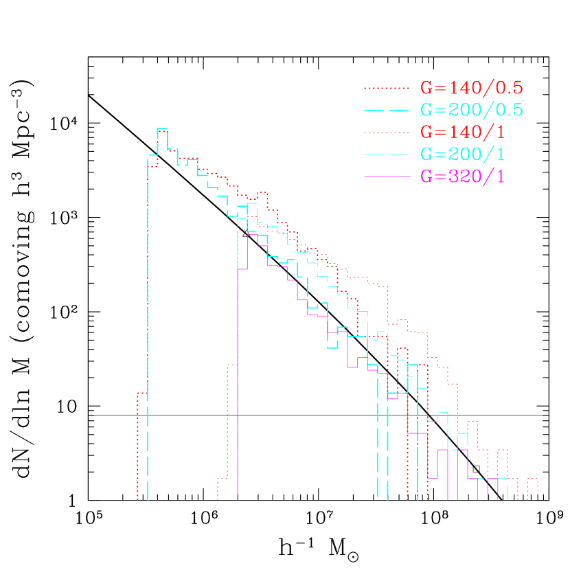
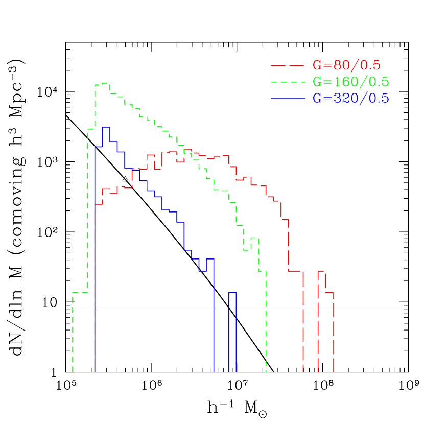
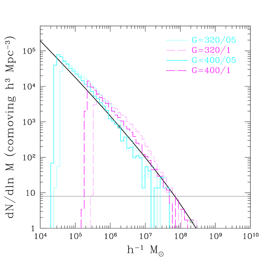
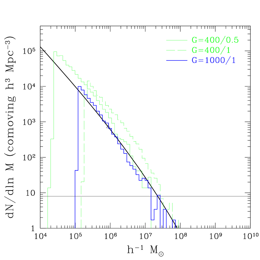
Figure 14: Comparison of the mass functions (histograms) varying the smoothing parameter $G$ and the Press-Schechter formalism with a top-hat filter (thick solid line). (Top-left) 64L05 and 64L1 at $z=11$ with $G=320,400$. (Top-right) 64L05 at $z=19$ with $G=80,160,320$. (Bottom-left) 128L05 and 128L1 at $z=12$ with $G=320,400$. (Bottom-right) 128L1 with $G=400$ and 256L1 with $G=1000$ at $z=15.13$.

References

- Abel et al. (1997) Abel, T., Anninos, P., Zhang, Y., & Norman, M. L. 1997, New Astronomy, 2, 181
- Abel et al. (2000) Abel, T., Bryan, G. L., & Norman, M. L. 2000, ApJ, 540, 39
- Bertschinger (1995) Bertschinger, E. 1995, GC-3 report, (astro-ph/9506070)
- Bertschinger & Gelb (1991) Bertschinger, E., & Gelb, J. M. 1991, Computers and Physics, 5, 164
- Black & Dalgarno (1976) Black, J. H., & Dalgarno, A. 1976, ApJ, 203, 132
- Brocato et al. (2000) Brocato, E., Castellani, V., Poli, F. M., & Raimondo, G. 2000, A&AS, 146, 91
- Brocato et al. (1999) Brocato, E., Castellani, V., Raimondo, G., & Romaniello, M. 1999, A&AS, 136, 65
- Bromm et al. (2001) Bromm, V., Kudritzki, R. P., & Loeb, A. 2001, ApJ, 552, 464
- Ciardi et al. (2000) Ciardi, B., Ferrara, A., Governato, F., & Jenkins, A. 2000, MNRAS, 314, 611
- Dove & Shull (1994) Dove, J. B., & Shull, J. M. 1994, ApJ, 430, 222
- Ferrara (1998) Ferrara, A. 1998, ApJ, 499, L17
- Galli & Palla (1998) Galli, D., & Palla, F. 1998, A&A, 335, 403
- Gnedin (1995) Gnedin, N. Y. 1995, ApJS, 97, 231
- Gnedin (1996) Gnedin, N. Y. 1996, ApJ, 456, 1
- Gnedin & Abel (2001) Gnedin, N. Y., & Abel, T. 2001, New Astronomy, 6, 437
- Gnedin & Bertschinger (1996) Gnedin, N. Y., & Bertschinger, E. 1996, ApJ, 470, 115
- Gnedin & Ostriker (1997) Gnedin, N. Y., & Ostriker, J. P. 1997, ApJ, 486, 581
- Haiman et al. (2000) Haiman, Z., Abel, T., & Rees, M. J. 2000, ApJ, 534, 11
- Haiman et al. (1996) Haiman, Z., Rees, M. J., & Loeb, A. 1996, ApJ, 467, 522
- Haiman et al. (1997) Haiman, Z., Rees, M. J., & Loeb, A. 1997, ApJ, 476, 458
- Kennicutt et al. (1989) Kennicutt, R. C., Edgar, B. K., & Hodge, P. W. 1989, ApJ, 337, 761
- Klypin et al. (1999) Klypin, A., Kravtsov, A. V., Valenzuela, O., & Prada, F. 1999, ApJ, 522, 82
- Larson (1998) Larson, R. B. 1998, MNRAS, 301, 569
- Leitherer et al. (1995) Leitherer, C., Ferguson, H. C., Heckman, T. M., & Lowenthal, J. D. 1995, ApJ, 454, L19
- Lepp & Shull (1983) Lepp, S., & Shull, J. M. 1983, ApJ, 270, 578
- Lepp & Shull (1984) Lepp, S., & Shull, J. M. 1984, ApJ, 280, 465
- Mac Low & Shull (1986) Mac Low, M.-M., & Shull, J. M. 1986, ApJ, 302, 585
- Machacek et al. (2001) Machacek, M. E., Bryan, G. L., & Abel, T. 2001, ApJ, 548, 509
- Madau et al. (1997) Madau, P., Meiksin, A., & Rees, M. J. 1997, ApJ, 475, 429
- Moore (1994) Moore, B. 1994, Nature, 370, 629
- Nakamura & Umemura (1999) Nakamura, F., & Umemura, M. 1999, ApJ, 515, 239
- Nakamura & Umemura (2001) Nakamura, F., & Umemura, M. 2001, ApJ, 548, 19
- Navarro & Steinmetz (2000) Navarro, J. F., & Steinmetz, M. 2000, ApJ, 538, 477
- Oh (2001) Oh, S. P. 2001, ApJ, 553, 499
- Press & Schechter (1974) Press, W. H., & Schechter, P. 1974, ApJ, 193, 437
- Ricotti et al. (2001) Ricotti, M., Gnedin, N. Y., & Shull, J. M. 2001, ApJ, 560, 580
- Ricotti et al. (2002) Ricotti, M., Gnedin, N. Y., & Shull, J. M. 2002, ApJ, submitted (Paper II astro-ph/0110432)
- Ricotti & Shull (2000) Ricotti, M., & Shull, J. M. 2000, ApJ, 542, 548
- Shapiro & Kang (1987) Shapiro, P. R., & Kang, H. 1987, ApJ, 318, 32
- Shull & van Steenberg (1985) Shull, J. M., & van Steenberg, M. E. 1985, ApJ, 298, 268
- Tegmark et al. (1997) Tegmark, M., Silk, J., Rees, M. J., Blanchard, A., Abel, T., & Palla, F. 1997, ApJ, 474, 1
- Tumlinson & Shull (2000) Tumlinson, J., & Shull, J. M. 2000, ApJ, 528, L65
- Uehara et al. (1996) Uehara, H., Susa, H., Nishi, R., Yamada, M., & Nakamura, T. 1996, ApJ, 473, L95
- Venkatesan et al. (2001) Venkatesan, A., Giroux, M. L., & Shull, J. M. 2001, ApJ, 563, 1
- Wood & Loeb (2000) Wood, K., & Loeb, A. 2000, ApJ, 545, 86