Hubble Space Telescope imaging of a peculiar stellar complex in NGC 6946

Abstract

The stellar populations in a stellar complex in NGC 6946 are analyzed on images taken with the Wide Field Planetary Camera 2 on board the Hubble Space Telescope. The complex is peculiar by its very high density of stars and clusters and semicircular shape. Its physical dimensions are about the same as for the local Gould Belt, but the stellar density is 1 – 2 orders of magnitude higher. In addition to an extremely luminous, $\sim 15$ Myr old cluster discussed in an earlier paper, accounting for about 17% of the integrated $V$-band light, we identify 18 stellar clusters within the complex with luminosities similar to the brightest open clusters in the Milky Way. The color-magnitude diagram of individual stars in the complex shows a paucity of red supergiants compared to model predictions in the 10–20 Myr age range for a uniform star formation rate. We thus find tentative evidence for a gap in the dispersed star formation history, with a concentration of star formation into a young globular cluster during this gap. Confirmation of this result must, however, await a better understanding of the late evolution of stars in the corresponding mass range ($\gtrsim 12$ M_⊙). A reddening map based on individual reddenings for 373 early-type stars is presented, showing significant variations in the absorption across the complex. These may be responsible for some of the arc-like structures previously identified on ground-based images. We finally discuss various formation scenarios for the complex and the star clusters within it.

1 Introduction

NGC 6946 is one of the nearest large spiral galaxies beyond the Local Group and has been scrutinized at nearly all wavelengths from X-rays (Schlegel, Blair, & Fesen, 2000), over optical and infrared studies (Bonnarel et al., 1988; Malhotra et al., 1996; Bianchi et al., 2000) to sub-millimeter (Tacconi & Young, 1989) and radio wavelengths (Boulanger & Viallefond, 1992; Ehle & Beck, 1993). The galaxy is classified as an Sc–type spiral, with a strong nuclear starburst (Engelbracht et al., 1996; Elmegreen, Chromey, & Santos, 1998) as well as a high level of star formation activity throughout the disk (Degioia-Eastwood et al., 1984; Sauty, Gerin, & Casoli, 1998). NGC 6946 has hosted 6 supernovae within the last century, another indication of vivid star formation in the galaxy (Schlegel, 1994). Its exact distance is still somewhat uncertain, partly because the galaxy is located at a relatively low galactic latitude ($b=12\deg$) and is subject to significant foreground extinction from our Galaxy. Burstein & Heiles (1984) give the reddening towards NGC 6946 as $A_{B}=1.62$ while the COBE/DIRBE maps by Schlegel et al. (1998) give a somewhat lower value of $A_{B}=1.48$. Throughout this paper we will adopt the latter value. For conversion between $B$-band extinction and other bands we use the reddening law by Cardelli, Clayton & Mathis (1989). The distance to NGC 6946 is listed as 5.5 Mpc in the Nearby Galaxies Catalogue (Tully, 1988), but more recent values are $5.9\pm 0.4$ Mpc (Karachentsev, Sharina & Huchtmeier, 2000), based on blue supergiants, or $5.7\pm 0.7$ Mpc (Eastman, Schmidt, & Kirshner, 1996) based on Type II supernovae. Here we use a distance of 5.9 Mpc to NGC 6946.

In spite of its relative proximity and numerous studies of NGC 6946 at many wavelengths, a peculiar stellar complex in one of its spiral arms has largely escaped attention since it was first discovered by Hodge (1967). Nevertheless, this object is quite conspicuous on optical images and was noticed by Larsen & Richtler (1999) on images taken with the 2.56 m Nordic Optical Telescope (NOT) during a search for young massive star clusters in nearby galaxies. The Hodge complex is host to one of the brightest young star clusters currently known in the disk of any spiral galaxy, with an estimated age of about 15 Myr and an absolute visual magnitude of $M_{V}=-13.2$ (Larsen et al., 2001, hereafter Paper II). It is located about 3 arc minutes (4.8 kpc) to the W of the galaxy center, at the end of a sub-branch of one of the main spiral arms. The complex is remarkable by its circular outer boundary, with a diameter of about $22\arcsec$ or $\sim 600$ pc. A color picture from the NOT, showing the location of the complex within NGC 6946, was presented by Elmegreen, Efremov & Larsen (2000, hereafter Paper I). In addition to the young “super–star cluster” (YSSC) they identified a number of other bright objects within the complex. Crowding problems and limited resolution on the ground-based images made it difficult to distinguish between clusters and individual luminous stars, but because of the high luminosities of many of these objects, they were assumed to be mostly star clusters. Rough age estimates were obtained from the $UBV$ colors, indicating ages similar to that of the YSSC.

On the NGC 6946 extinction map by Trewhella (1998), the complex can be identified as a “cavity” of reduced extinction, presumably because star formation has cleared out much of the obscuring material. However, significant variations in the integrated $V-I$ color across the surface of the region can still be seen, presumably an indication of considerable reddening variations (Paper I). This might also explain – at least partly – a number of arc-like features noted by Hodge (1967), who suggested that the origin of these arcs might be related to “super-super nova” explosions (Shklovsky, 1960), and that the apparently similar structures in the LMC Constellation III might have originated in the same way. This possibility has been further discussed by Efremov et al. (2001). The $7\mu$ and $15\mu$ ISOCAM maps by Malhotra et al. (1996) show hints of the complex, but it is not apparent on 450$\mu$ and $850\mu$ JCMT/SCUBA data (Bianchi et al., 2000). A CO map (Tacconi & Young, 1989) of the central $6\farcm 75$ of NGC 6946 shows a region of enhanced CO density, corresponding to the spiral arm in which the complex is located, but higher-resolution CO data (Walsh et al., in preparation) do not show a particularly high CO density in the vicinity of the complex. Kamphuis (1993) identified a number of HI holes in the disk of NGC 6946 on high-resolution (15″) HI maps, possibly cleared by star formation. Many of these HI holes are located in the western part of the galaxy, but none of them coincides with the exact location of the complex. Thus, while much of the original molecular gas may have been consumed and/or dissociated by star formation, the complex does not yet appear to have caused a significant hole in the HI disk around it. The NOT data also show isolated regions of H$\alpha$ emission near the center of the complex and along the rim, coincident with the regions of enhanced absorption (Paper I), indicating that some star formation may still be taking place in the complex or at least that it has proceeded until very recently.

In this paper we analyze new images of the complex, taken with the Wide Field Planetary Camera 2 (WFPC2) on board the Hubble Space Telescope (HST). A color image of the complex and its surroundings, generated from our WFPC2 images, is shown in Figure 1. In Paper II we have used these data to study the young massive cluster that dominates the complex and we now turn to the numerous other objects, including a number of other clusters and the field stars. We present a color-magnitude diagram for stars in the complex and analyze its recent star formation history, probably making NGC 6946 one of the most distant galaxies for which such an analysis has been attempted. We also discuss possible formation scenarios.

2 Data reduction

The data were obtained in Cycle 9 and consist of integrations in the F336W ($U$), F439W ($B$), F555W ($V$) and F814W ($I$) bands with exposure times of 3000 s, 2200 s, 600 s and 1400 s, respectively. Shorter integrations in each band were also obtained, in case the central pixels of the main cluster would be saturated. However, the cluster turned out to be extended enough that this was not a problem and hence these shorter integrations were not used. A 300 sec exposure in F656N was also taken to trace H$\alpha$ emission. The entire complex is comfortably contained within the $36\arcsec\times 36\arcsec$ field of the Planetary Camera (Fig. 2) and we only consider data in the PC chip in this paper. The pixel scale of $0\farcs 045$ per pixel corresponds to 1.29 pc at the adopted distance.

Initial processing of the images were performed “on-the-fly” by the standard calibrating pipeline at STScI. Subsequently, the YSSC was subtracted from the images using the ELLIPSE task in the STSDAS package, allowing photometry to be obtained for fainter objects near the cluster. Objects were detected on a sum of the F555W and F814W images using the DAOFIND task in the DAOPHOT package, running within IRAF, using a $3\sigma$ detection threshold. Aperture and PSF-fitting photometry was then obtained by the PHOT and ALLSTAR tasks in DAOPHOT, using a two-iteration procedure whereby additional objects were detected during a second pass of DAOFIND on the object-subtracted image generated by the first run of ALLSTAR (Stetson, 1987). For the ALLSTAR photometry, the PSF was empirically determined using stars in uncrowded regions.

The $V$ and $I$ data were far deeper than the $B$ and $U$ data, but many of the brighter objects in the field nevertheless had adequate photometry in all four bands. Extensive completeness tests were done for the $V$ and $I$ PSF photometry, by populating the PC image with artificial stars having magnitudes between $V=19.0$ and $V=27.5$ at 0.5 mag intervals, and with $V\!-\!I$ colors between $-1.0$ and $+4.0$ at 1.0 mag intervals. For each $V,\mbox{$V\!-\!I$}$ combination, 4 completeness tests with 500 artificial stars each were done. The stars were added at random positions within the central $600\times 600$ pixels of the PC frame, but with required separations larger than 10 pixels. Thus, the completeness was determined as a function of both $V$ magnitude and $V-I$ color, which is essential in a case like this where the objects span a wide range in color.

Aperture photometry was obtained both in an $r=3$ pixels aperture and in an $r=11$ pixels (0$\farcs$5) aperture. The aperture photometry was used mainly for extended objects, measuring colors in the smaller aperture (to minimize random errors) while the $r=11$ aperture was used for cluster magnitudes to reduce the uncertainty on the aperture correction for extended objects. The photometry was calibrated to standard $UBVI$ magnitudes using the relations in Holtzman et al. (1995), which refer to a $0\farcs 5$ ($r=11$ pixels) aperture. Aperture corrections between the $r=3$ pixels and $r=11$ apertures (Table 1) were determined from aperture photometry on synthetic images, generated by convolving the TinyTim PSF (Krist & Hook, 1997) with the WFPC2 “diffusion kernel”. For $B$, $V$ and $U$ the aperture corrections from $r=3$ to $r=11$ pixels apertures were essentially identical (to within about 0.01 mag), while the correction for the $V\!-\!I$ colors amounts to 0.06 mag. The zero-points for the PSF-fitting photometry were established by comparison with the aperture photometry and the subsequent calibration to the standard system was done in the same way as for the aperture photometry.

In order to classify objects as clusters or individual stars, sizes were measured for all objects by use of the ishape algorithm (Larsen, 1999). This algorithm estimates intrinsic object sizes by convolving an analytic model of the object shape with the PSF, adjusting the FWHM of the model until the best possible match with the observed profile is obtained. In this way, sizes can be reliably measured even for sources that have significantly smaller intrinsic sizes than the PSF. Here we have assumed King profiles with a concentration parameter $c=$ r(tidal) / r(core) = 30 for the intrinsic object profiles and PSFs generated by TinyTim. The modeling also includes a convolution with the WFPC2 diffusion kernel. Alternatively, we could have used e.g. the ALLSTAR sharpness estimate to identify extended objects. A comparison of the ALLSTAR sharpness parameter and ishape FWHM estimates for objects in the PC frame showed that the two methods yielded consistent results in most cases, although objects that were clearly recognized as extended by ishape would occasionally be classified as point sources by ALLSTAR. In such cases, visual inspection of the images and measurements of their FWHM values with the IMEXAMINE task in IRAF would generally support the ishape measurements. For a detailed description of ishape and tests of its performance, we refer to Larsen (1999) and Larsen, Forbes & Brodie (2001).

3 Results

Figure 2 shows the PC field of view, with the young super-star cluster clearly visible as the brightest object in the field, near the center of the image. Within a radius of $r=300$ pixels from the center of the image, the complex has a total integrated magnitude of $V=15.0$ (including the YSSC), corresponding to $M_{V}=-15.0$. With $M_{V}=-13.2$ (Paper II), the cluster thus accounts for about 17% of the total $V$-band light that we receive from the complex. This calculation does not account for the fact that significant absorption is likely to be present, obscuring some fraction of the light, so in practice the cluster may contribute with a smaller fraction of the total light from the complex. Considering that the cluster has a mass around $10^{6}M_{\odot}$ (with estimates ranging from $5\times 10^{5}\mbox{${\rm M}_{\odot}$}$ to $(1.7\pm 0.9)\times 10^{6}\mbox{${\rm M}_{\odot}$}$, see Paper II), the whole complex probably has a mass of $\sim 10^{7}\mbox{${\rm M}_{\odot}$}$. However, the uncertainty on this number is considerable and the mass could range between a few times $10^{6}$ ${\rm M}_{\odot}$ and well above $10^{7}$ ${\rm M}_{\odot}$.

3.1 Separating clusters and stars

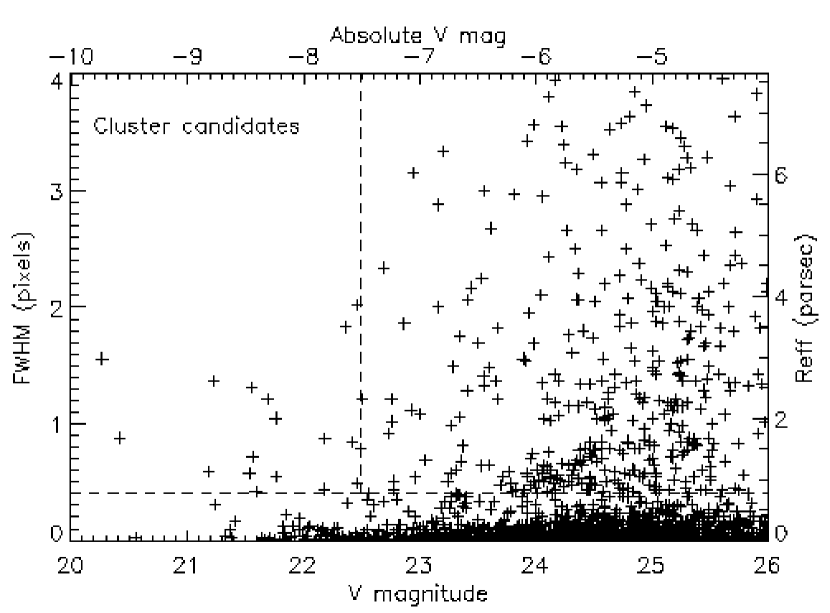
Figure 3: Object size as a function of $V$ magnitude for all objects in the PC frame. Stellar objects are selected as objects with FWHM $<\mbox{$0.4$}$ pixels.

Figure 3 shows the intrinsic object sizes as a function of $V$ magnitude, measured in the $r=3$ pixels aperture. Individual stars are distributed in a narrow range of FWHM values $\lesssim 0.3$ pixels, while clusters have larger FWHM values. Reliable size measurements require a S/N $\sim 30$ (Larsen, 1999), corresponding to $V\sim 22.5$. Comparing object sizes measured on F555W and F814W images, we found a scatter of about 0.2 pixels around a 1:1 relation for objects brighter than $V=22.5$, with no evident systematic differences between the two sets of measurements. This scatter is similar to the width of the strip defined by point sources near the $x$-axis in Fig. 3, and is also consistent with previous estimates of the accuracy by which ishape can measure sizes (e.g. Larsen, Forbes & Brodie, 2001). Thus, we estimate that the size measurements are accurate to about 0.2 pixels for $V<22.5$. Below this limit, much of the scatter in FWHM in Fig. 3 is likely due to measurement errors but for the brighter objects one can clearly distinguish between extended sources (likely clusters) and point sources (stars).

It is evident from Fig. 3 that some individual stars as bright as $M_{V}\approx-8.5$ are present in the field, making distinction between stars and clusters based on luminosity alone infeasible. We select cluster candidates as objects with FWHM$>$$0.4$ pixels, corresponding to an effective (half-light) radius larger than 0.8 pc. From the above considerations concerning the accuracy of our size measurements, this adopted size cut allows us to confidently identify a list of extended objects. We further impose a magnitude limit of $V=22.5$ ($M_{V}=-7.5$) as measured in the $r=3$ pixels aperture, resulting in 18 cluster candidates. The $V=22.5$ cut-off is motivated partly by the need for adequate S/N for reliable size measurements, and partly by the fact that it becomes increasingly difficult to distinguish between real clusters and simple blends due to crowding at fainter magnitudes. The cluster candidates selected in this way are indicated in Figure 2 and integrated photometry is given in Table 2, which also gives integrated colors and magnitudes for the whole complex measured in an $r=300$ pixels aperture and for the YSSC (from Paper II). The bright object near cluster #2848 is unresolved on the HST image and is probably a Galactic foreground star (Paper I). Most of the 18 objects selected according to the above criteria are probably genuine clusters, although the census may not be complete. It is clear from Fig. 3 that a fainter magnitude limit and/or smaller size cut would lead to more cluster candidates, but we have chosen relatively conservative size/magnitude cuts to reduce the risk of including blends of stars in crowded regions. Also, our selection criteria do not include more extended groupings of stars (such as the fuzzy object next to cluster #2284), but these are unlikely to be bound clusters.

The $V$ band magnitudes in Table 2 are measured in the $r=11$ pixels aperture, making them less sensitive to size-dependent aperture corrections. 11 of the clusters have $M_{V}$ brighter than $-9$ and two objects are brighter than $M_{V}=-10$. Although they appear relatively inconspicuous in comparison with the YSSC, these clusters are actually comparable in luminosity to the brightest open clusters in the Milky Way. Most of them were also identified in Paper I, but some of the fainter sources identified in that paper are probably individual luminous stars or chance alignments of several stars, which were unresolved on the ground-based images.

A $(\bv,\ub)_{0}$ two-color diagram for objects brighter than $V=22.5$ is shown in Figure 4. Clusters are shown with $+$ markers while stars are shown with diamond ($\diamond$) symbols. The plot also includes two solar-metallicity stellar isochrones for ages of 4 Myr and 10 Myr from Girardi et al. (2000) and the Girardi et al. (1995) ‘S’-sequence, representing the average colors of LMC clusters. The arrow indicates the effect of a reddening of 0.5 in $E(\bv)$. The S-sequence is basically an age sequence, with ages increasing along the sequence from blue to red colors. Stars and clusters clearly have different color distributions, with most of the clusters scattering along the S-sequence while stars occupy a wider range in colors, giving confidence to the selection criteria. Although the cluster candidates are mostly distributed along the S-sequence, the direction of scatter is also nearly parallel to the reddening vector. Thus, the scatter in cluster colors can be caused by age differences, by differences in the absorption, or a combination of the two. An additional source of scatter in the cluster colors comes from stochastic color variations, because much of the integrated light is dominated by a small number of very luminous stars (Girardi et al., 1995). The latter effect becomes more severe for the fainter clusters.

Another potential age indicator is the reddening-free $Q_{1}$ parameter, $Q_{1}=(\ub)-0.69(\bv)-0.05(\bv)^{2}$ (Cardelli, Clayton & Mathis, 1989; Harris, Zaritsky, & Thompson, 1997). Figure 5 shows model predictions for the evolution of $Q_{1}$ as a function of age, using population synthesis models from Bruzual & Charlot (2001). The models are shown for three different metallicities, $Z=0.02$ (solar), $Z=0.008$ and $Z=0.004$. From Table 2, most clusters have $Q_{1}$ values between $-0.9$ and $-0.6$. By comparison with Figure 5, it is clear that the clusters are all young objects, but the $Q_{1}$ index varies in an essentially random manner as a function of age below log(age)$\approx$7.2, with a strong dependence on metallicity as well. Thus, the cluster ages are not well constrained.

3.2 Constructing a reddening map

A reddening map of the Hodge complex was presented in Paper I, based on its integrated $V\!-\!I$ colors. Although that map showed evidence for significant reddening variations, it relied on the assumption that color variations were due to differential reddening of a background illumination of constant color. With the HST data, this analysis can now be refined by obtaining reddenings for individual early-type stars.

In order to determine reddenings for individual stars, we again use the $Q_{1}$ parameter. For $Q_{1}<0$, the relation between $Q_{1}$ and $(\bv)_{0}$ can be approximated as $\mbox{$(\bv)_{0}$}=0.32\,Q_{1}-0.024$ (read off Fig.2 in Harris, Zaritsky, & Thompson, 1997). Our adopted reddening law is slightly different from the one used by Harris, Zaritsky, & Thompson (1997), but comparison with stellar models from Girardi et al. (2000) shows that this hardly affects the relation between $Q_{1}$ and $(\bv)_{0}$. Thus, by comparing the observed B V color of a star with its intrinsic color $(\bv)_{0}$ determined from the reddening-free $Q_{1}$, the color excess $E(\bv)=(\bv)-\mbox{$(\bv)_{0}$}$ can be established, and the $B$-band absorption is then $A_{B}=4.0\,E(\bv)$.

In this way, individual $A_{B}$ values were determined by using the PSF photometry for all point sources with errors in U B and B V less than 0.3 mag, $\mbox{$(\ub)_{0}$}<0$ (only corrected for foreground extinction) and $Q_{1}<0$. A total of 373 stars satisfied these criteria. The B V and U B error limits of 0.3 correspond to an error of 0.38 in $E(B-V)$ or about 1.5 magnitudes in $A_{B}$ for any individual star, which is on the same order of magnitude as the total scatter in the observed reddenings. Even though the 0.3 mag are an upper error limit and some stars will have smaller errors than this, it is necessary to obtain the reddening estimate at any given point in the image as an average of several individual measurements. We generated our reddening map by convolution of the individual measurements with an Epanechnikov kernel with a smoothing radius of 30 pixels. Since most of the stars are contained within a radius of $\sim 200$ pixels from the center, this means that an average of about 10 individual measurements is used at each point in the map, making it possible to detect variations in $A_{B}$ at about the 0.5 mag level. Narrowing down the error limits leads to smaller errors on any individual $A_{B}$ value, but also decreases the number of sampling points.

The resulting reddening map is shown in Figure 6. Red and blue colors indicate high and low reddening, respectively. The reddening scale is indicated by the wedge at the bottom of the figure, which spans a range between $A_{B}=1.5$ and $A_{B}=3.5$ in total extinction, i.e. the map shows a range of $A_{B}=0.0-2.0$ in internal $B$-band absorption. Compared to the Paper I reddening map, Figure 6 shows the same main features: Areas of increased reddening along the outer arc and near the dark clouds north (left) of the bright cluster, and lower absorption to the southwest (above and to the right). Most features outside the main complex, where the stellar density is low, are probably just artifacts. Roughly speaking, whenever the circular shape of the convolution kernel is present, this means that the reddening value within that region of the map is based on only one star, and should therefore be interpreted with caution.

As a test of the reality of the features seen in Figure 6, we generated similar maps, but using $V\!-\!I$ colors instead of B V colors to get the color excess. Another test was done by randomly dividing the stars into two samples and generating reddening maps for each sample. All the main features were consistently reproduced by the various methods: Increased reddening along the outer arc and near the dark clouds, and decreased reddening to the southwest. The agreement with the Paper I reddening map lends further support to the idea that many of the apparent structures in the complex are (at least partially) due to obscuration. In this respect, this complex may be quite different in nature from the peculiar arcs in e.g. the LMC Constellation III, where absorption probably plays only a minor role.

3.3 Modeling of the color-magnitude diagram

As discussed in Section 3.1, ages of stellar clusters are uncertain because of stochastic color variations, variable reddening etc. The small number of clusters, age fading and dynamical evolution represent further difficulties when using clusters as tracers of the star formation history (SFH). However, information about the SFH can also be inferred from the numerous field stars that are present in the complex.

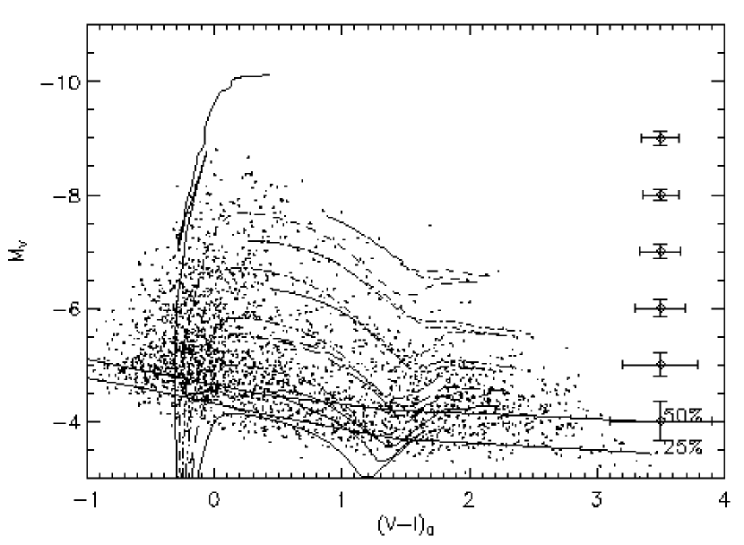
Figure 7: ($\mbox{$(V\!-\!I)_{0}$},M_{V}$) color-magnitude diagram for PSF-fitting photometry for point sources in the PC frame. Stellar isochrones for ages of 4, 10, 16, 25, 40 and 63 Myr from Girardi et al. (2000) are superposed on the plot. The 50% and 25% completeness limits are also shown.

Figure 7 shows a $V,\mbox{$(V\!-\!I)_{0}$}$ color-magnitude diagram (CMD) for PSF photometry of point sources, with the 50% and 25% completeness limits indicated. The blue part of the CMD is dominated by a combination of main-sequence (MS) stars and blue supergiants as bright as $M_{V}\sim-9$, while red supergiants appear at $M_{V}\approx-6$ with most of them being fainter than $M_{V}=-5$. The plot also includes solar-metallicity stellar isochrones from the Padua group (Bertelli et al., 1994; Girardi et al., 2000) for ages of 4, 10, 16, 25, 40 and 63 Myr. It is clear that the entire CMD cannot be adequately represented by a single isochrone and the red supergiants (RSGs) appear to be significantly older than the most luminous blue stars, indicating an age spread within the complex.

Rough estimates of the expected contamination from Galactic stars can be obtained from Ratnatunga & Bahcall (1985). They do not list data for NGC 6946 specifically, but we can use their calculations for NGC 2808 which is located at $b=-11\deg$ and $l=282\deg$. As their model assumes symmetry around the Galactic plane and with respect to $l=0\deg$, this is equivalent to a position about $20\deg$ closer to the Galactic center than NGC 6946 and slightly closer to the plane, i.e. this field should slightly overestimate the contamination. For $\bv<1.3$, Ratnatunga & Bahcall (1985) predict less than 1 star with $21<V<27$ within the PC field. For $\bv>1.3$, 8 stars with $25<V<27$, 5 stars with $23<V<25$ and 2 stars with $21<V<23$ are predicted. Using Padua models and correcting for foreground extinction, the $\bv=1.3$ limit corresponds to $\mbox{$V\!-\!I$}\sim 1.3$. Counting the number of stars with $\mbox{$V\!-\!I$}>1.3$ in our CMD, we find that the expected contamination rate is $\sim 1\%$ for $V$ fainter than 23 and $\sim 3\%$ for $V$ brighter than 23. Clearly, contamination by foreground stars is negligible.

Figure 8 illustrates the spatial distributions of early-type stars brighter than $V=23.5$ ($M_{V}=-6.5$) (left) and for RSGs (right). Here we have selected “early-type” stars as stars with $\mbox{$V\!-\!I$}<1.0$ and RSGs as stars with $\mbox{$V\!-\!I$}>1.5$. As this division is essentially one by age, the two maps can be used to compare the distributions of the youngest and slightly older stars in the complex. Both maps show a concentration towards the center of the complex, indicating that both populations are indeed associated with the complex. The two dark clouds near the center can be clearly seen as “voids” in the spatial distribution of blue stars. Generally, the outer boundary of the region occupied by these stars is fairly well defined. For the RSGs, the spatial distribution is more diffuse, as expected for an older population that has had more time to migrate away from the original birth locations.

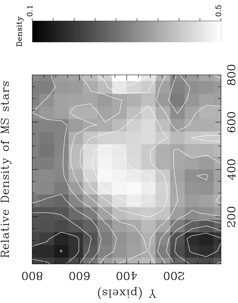
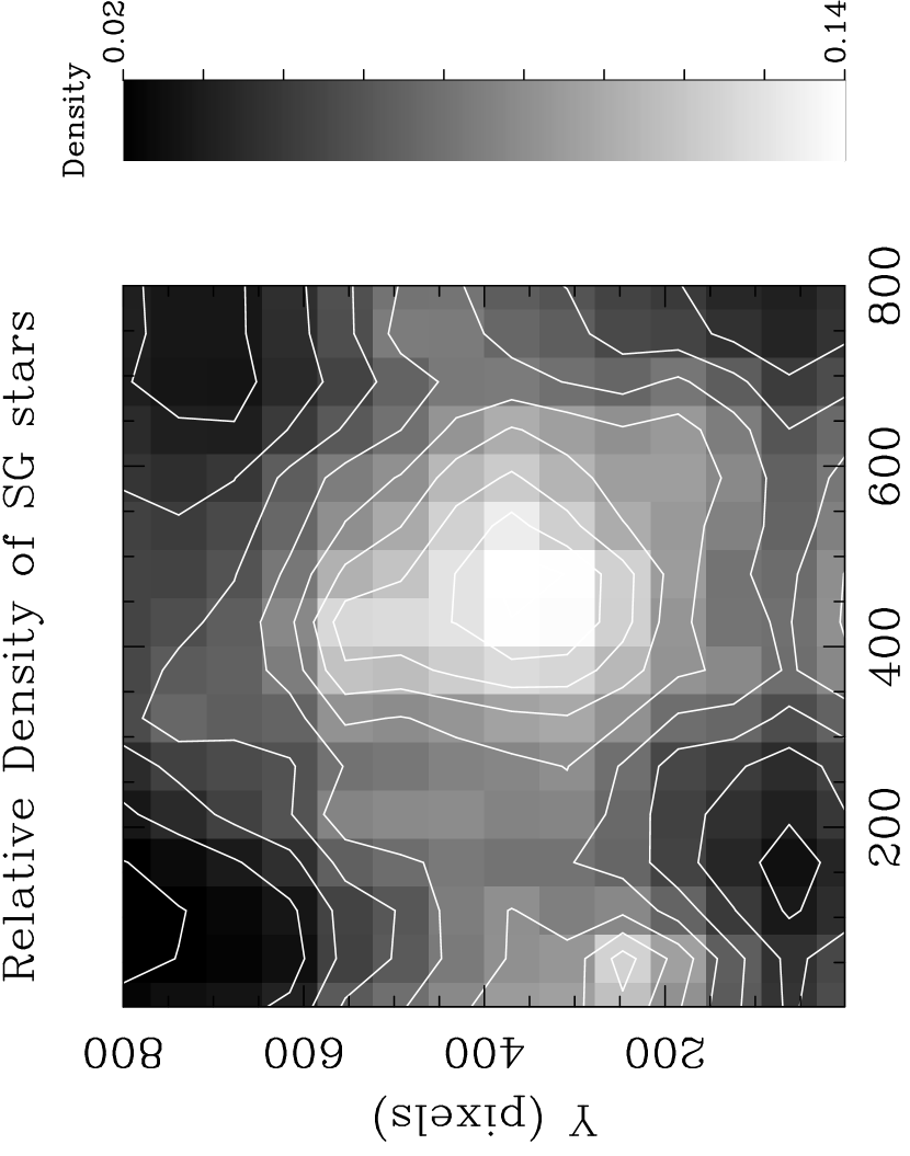
Figure 9: Relative density distributions for early-type and red supergiant (RSG) stars. As in Fig. 8, the maximum in the relative number density of red stars is offset from that of the blue stars and coincides with the center of curvature of the western rim.

The maps in Fig. 8 may be affected by the distribution of external extinction, sampling and completeness of the photometry. In order to reduce these effects, we also generated density maps showing the relative densities of blue and red stars, normalized to the total number of stars at each position (Figure 9). Again, these maps show a concentration of both red and blue stars towards the center of the complex, although the density maximum of the red population has now shifted toward the higher $X$-values. This may, however, be an artifact of the normalization procedure, since the number of blue stars is lower there.

In the following we will attempt to gain some further insight into the recent star formation history of the complex by reconstructing its color-magnitude diagram, using the Padua set of isochrones. The goal is to find a combination of isochrones which, when combined, provides a match to the observed color-magnitude diagram, and then infer the star formation history (SFH) from the relative weights of the isochrones.

3.3.1 Technique

The basic idea behind such modeling is that the relative fractions of stars of different ages vary from one part of the color-magnitude diagram to another. Thus, by counting the number of stars in various parts of the color-magnitude diagram and comparing with model predictions, the combination of stellar isochrones which best fits the observed number counts can be determined. Some early attempts to model the star formation history of CCD fields in the LMC in this way were done by Bertelli et al. (1992), who simply compared the relative numbers of red clump and main sequence stars, enabling them to constrain the relative SFR for young stars (dominating the upper main sequence) and $\sim 4$ Gyr old stars (dominating the red clump). More sophisticated techniques have since been employed for the LMC (e.g. Holtzman et al., 1999; Olsen, 1999; Dirsch et al., 2000; Dolphin, 2000; Harris & Zaritsky, 2001) and other Local Group galaxies (Gallart et al., 1999; Wyder, 2001), dividing the CMD into finer grids and/or utilizing photometry in multiple bands. As discussed in these papers, great care must be taken when interpreting the results from such modeling, since different assumptions about reddening, distance, metallicity, stellar IMF, binary fraction and other factors can lead to significantly different results. Furthermore, the models of massive stars are still very uncertain and have well-documented problems in matching the observed CMDs of luminous stars in the Milky Way as well as the LMC (e.g. Chiosi, 1998). With these precautions in mind, we nevertheless proceed to attempt a reconstruction of the CMD for the complex in NGC 6946.

The isochrones were downloaded from the WWW site of the Padua group and are based on Girardi et al. (2000) stellar models for masses up to 8 ${\rm M}_{\odot}$ and on Bertelli et al. (1994) models for more massive stars. For each individual isochrone a set of synthetic ($V,I$) datapoints was generated, corresponding to masses between 100${\rm M}_{\odot}$ and a lower limit of 4${\rm M}_{\odot}$, below the observational cut-off. Unless otherwise noted, the masses were distributed according to a Salpeter (1955) stellar IMF. The $V$ and $I$ magnitudes for a given mass and age were obtained by interpolation in the isochrone and adding an optional offset to simulate reddening. Datapoints corresponding to masses above the endpoints of stellar evolution were simply assigned a luminosity of 0, thereby not contributing to the CMD, but still being counted for normalization purposes. Photometric errors were then added to each datapoint by adding random offsets to the $V$ and $I$ magnitudes, scaled to the photometric errors of the closest star in the observed CMD. Finally, the synthetic data were de-populated according to the completeness function determined for the observations. Because of brighter completeness limits in $B$ and $U$, we only used the $V$ and $I$ data for this modeling.

For the purpose of evaluating the “goodness” of the fit to the observed CMD provided by a modeled CMD we chose the $\chi^{2}$ statistic, comparing the number of stars in the synthetic and observed CMDs within a number of “$\chi^{2}$ boxes”. We compared the number of stars observed in the $i$th $\chi^{2}$ box (${\rm Cnt}_{i,{\rm data}}$) with the density of synthetic datapoints in the same box (${\rm Cnt}_{i,{\rm synt}}$), obtained by summing the contributions from each isochrone (${\rm Cnt}_{ij,{\rm synt}}$). The best fit was then defined as the one minimizing the function

$$\chi^{2}(W)=\frac{1}{N_{\rm bx}}\sum_{i=1}^{N_{\rm bx}}\frac{\left({\rm Cnt}_{i,{\rm data}}-c\,\sum_{j=1}^{N_{\rm iso}}W_{j}{\rm Cnt}_{ij,{\rm synt}}\right)^{2}}{{\rm Cnt}_{i,{\rm data}}+1}$$ (1)

where $N_{\rm bx}$ is the number of $\chi^{2}$ boxes, $N_{\rm iso}$ is the number of isochrones, $c$ is a normalization constant and $W_{j}$ are the weights of the isochrones. The addition of 1 to the denominator is just a convenient way to avoid division by zero for empty boxes.

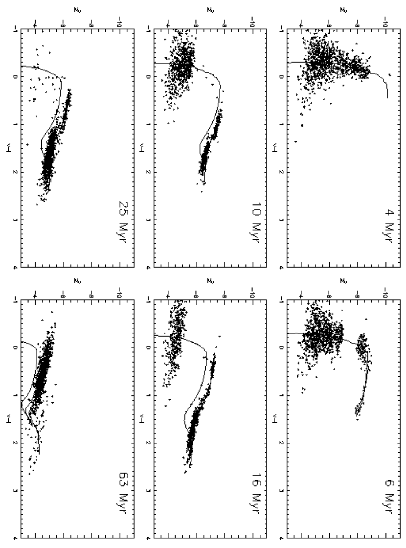
Figure 10: Simulated color-magnitude diagrams for stellar populations of six different ages, based on Padua isochrones. The isochrones have been populated according to a Salpeter IMF. Using the data corresponding to our NGC 6946 photometry, photometric errors have been added and the diagrams have been depopulated according to the completeness functions. Each plot contains 1000 points.

Figure 10 illustrates the first steps in this process: each of the six panels in the figure shows the CMD for a single isochrone after addition of photometric errors. None of the panels in Fig. 10 provides a match to the observed color-magnitude diagram, which contains a combination of very luminous blue stars only present in the youngest isochrones, as well as red supergiants belonging to a somewhat older ($\sim 25$ Myr) population. Each of the plots in Figure 10 contains 1000 stars, but the synthetic CMDs used for the fits were populated with many more stars in order to eliminate the effects of Poisson statistics in the synthetic data. Specifically, about $3\times 10^{5}$ synthetic datapoints were generated for each isochrone.

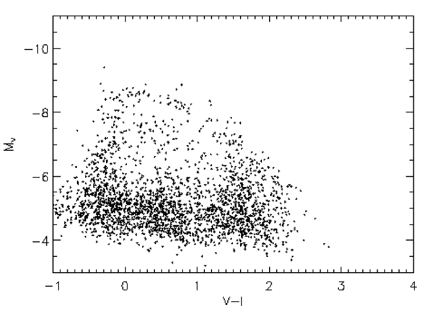
Figure 11: Simulated color-magnitude diagram for constant star formation rate in the range 4.0 – 100 Myr, using Padua $Z=0.019$ isochrones.

Figure 11 shows a synthetic color-magnitude diagram for a constant star formation rate from 4 to 100 Myr. The upper age limit is not important; above $\sim 50$ Myr only few stars are brighter than the completeness limit. This synthetic CMD is already a much better match to the observed one, although some important differences remain. There are now too few luminous early-type stars and too many RSGs brighter than $M_{V}\sim-5$. By comparison with Fig. 7, this suggests that the youngest isochrones should be weighted more strongly, and isochrones at intermediate ages (10–20 Myr) should carry less weight.

The Padua isochrones are tabulated at intervals of 0.05 in log(age), making Eq. (1) a function of 29 variables for a range of 6.6–8.0 in log(age). In practice, this was a prohibitively large number of free parameters to fit at one time, so to make the problem more manageable we divided the isochrones into a number of groups, fitting all isochrones within a group together. The separations between the groups were set at log(age) = 6.7, 6.85, 7.0, 7.15, 7.3, 7.5, and 7.7. The $\chi^{2}$ minimization was done with the downhill simplex algorithm as described in Numerical Recipes (Press et al., 1992). Because the algorithm has a known tendency to get stuck at local minima, we followed the recommended procedure of restarting it once it claimed to have found a minimum. A stable minimum would typically be reached after 3–4 restarts. As an additional safety precaution against reaching only a local minimum, each simulation involved running the algorithm 5 times with different initial guesses for the fitted parameters (a constant SFR, constant weights, and three randomly selected combinations of weights for each group). In general, the final result did not depend strongly on the initial guesses.

Our algorithm allowed the $\chi^{2}$ boxes to be user-defined. Ideally, one would hope to obtain a perfect fit between the simulated and observed data at any point in the CMD, but in reality this is not possible. Depending on how the boxes were defined, we could regulate the sensitivity of the results to various effects: For example, very broad boxes would reduce the influence of reddening effects. Also, a cruder division was used to fit the red supergiants, since the colors and relative numbers of these are more uncertain. In practice, the boxes were chosen in a trial-and-error manner, by adjusting the number of boxes and the color/magnitude range covered by each box until the algorithm succeeded in producing a synthetic CMD that resembled the observed CMD as closely as possible.

3.3.2 Star formation history

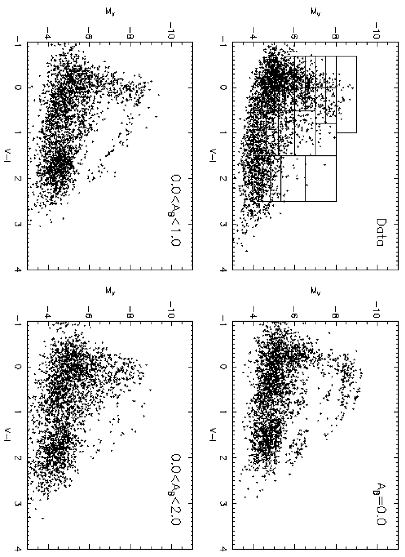
Figure 12: Simulated color-magnitude diagrams for three different reddening distributions. The stars were assigned random reddenings in the given intervals.

The best-fitting synthetic CMDs are shown in Figure 12. The upper-left panel shows the actual data and the $\chi^{2}$ boxes, while the remaining three panels show synthetic CMDs for different assumptions about the internal reddening: No reddening ($A_{B}=0$) and random reddenings in the intervals $0<A_{B}<1$ and $0<A_{B}<2$. Details about the fits are listed in Table 4. Each plot contains the same number of stars as the observed CMD. The $A_{B}=0$ synthetic CMD clearly provides a poor match to the observations and is unable to reproduce the broad color distribution of the early-type stars, no matter how the star formation history is fine-tuned. Visually, the $0<A_{B}<2$ plot appears to provide the best match, but the $\chi^{2}$ is actually lower for the $0<A_{B}<1$ plot. In any case, these simulations again show that significant reddening is present in the complex.

Instead of assigning random reddenings to the model CMDs, we could also have used the reddening map (Figure 6) to de-redden the data. However, a color-magnitude diagram for photometry de-reddened by means of the reddening map did not appear significantly different from a CMD where a uniform reddening was assumed, presumably because the reddening map only gives an average reddening at each point and does not contain information about the scatter at any given position. We thus decided to follow the simpler approach of assigning random reddenings to the simulated CMDs.

Figure 13 shows the star formation histories corresponding to the three synthetic CMDs in Figure 12. The relative star formation rate at each age is simply the weight $W_{j}$ divided by the spacing in age between the isochrones at that age. Each curve has been normalized to give a total stellar mass of $10^{7}$ ${\rm M}_{\odot}$ over the past 50 Myr. The YSSC is represented by the Gaussian curve at 15 Myr, assuming a cluster mass of $10^{6}$ ${\rm M}_{\odot}$. The curve has a FWHM of 2 Myr, corresponding to the cluster crossing time for a diameter of 20 pc and velocity dispersion 10 km/s (Elmegreen, 2000).

Although the details clearly depend on the reddening assumption, all three SFHs show the same qualitive features: A recent burst of star formation, starting at about 6 Myr and continuing up until the lower age limit of the isochrones, a period of essentially no star formation between 6 Myr and 15–20 Myr (except for the YSSC), and an older burst. Beyond 30 Myr or so the results become very uncertain, as even the brightest stars are near the detection limit.

3.3.3 Spatial variations in the SFH

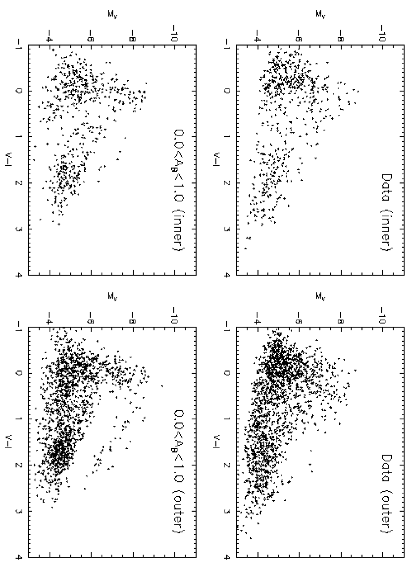
Figure 14: Observed and simulated color-magnitude diagrams for the central 100 pixels (left) and for $100<r<300$ pixels (right).

In an attempt to detect any differences in the SFH between the inner and outer parts of the complex, which might provide hints to its origin, we performed the CMD modeling analysis for the central 100 pixels and for $100<r<300$ pixels separately (see Figure 2). The observed and best-fitting synthetic CMDs for the two zones are shown in Figure 14 and the corresponding star formation histories are plotted in Figure 15. The normalizations of the respective SFHs are arbitrary. Figure 15 suggests slightly different SFHs for the two zones: The recent burst seems to be somewhat stronger in the central parts, and the intermediate quiescent period may have been briefer here. The older burst overlaps with the age of the young super-star cluster, and it seems likely that the cluster formed near the end of this initial burst of star formation. Although we have argued above that the results are very uncertain for ages older than $\sim 30$ Myr, the smaller relative SFR at ages $\gtrsim$ 30 Myr in the central zone is compatible with the oldest stars belonging to a general field population whose relative contribution is smaller in the more densely populated central parts. However, to first order the entire complex appears to have had a quite uniform star formation history.

3.3.4 Uncertainties

As already mentioned, the results can be quite sensitive to the various input assumptions. A shallower IMF slope, for example, leads to a weaker 6 Myr burst, because a star forming event of any given strength produces larger numbers of high-mass stars. We also tried varying the distance modulus by 0.5 mag to either side of the assumed value (28.4 and 29.4) but found no strong effect on the results. Again, the best solution would be obtained for a star formation history with an initial burst, followed by a quiescent period and a second burst.

The lower age limit of the Padua isochrones is 4 Myr, effectively truncating our simulated SFHs at ages below 4 Myr or about half the estimated age of the onset of the second burst. If star formation is continuing until the present day in the complex then even younger stars would also contribute to the CMD, and the average relative SFR of the youngest burst would be correspondingly lower.

A more critical ingredient in the modeling is the stellar isochrones. The Padua group also provides lower-metallicity models ($Z=0.008$ and $Z=0.004$), but for these lower metallicities the red supergiants are too blue to be compatible with the observed CMD. Thus, the only isochrones that allow us to obtain an acceptable fit to the data are the solar-metallicity ones. The abundances of various elements in HII regions in NGC 6946 have been studied by McCall, Rybski, & Shields (1985) and Ferguson, Gallagher, & Wyse (1998). The galaxy shows a clear abundance gradient as a function of distance from the center, but at the distance of the stellar complex discussed in this paper both studies find Oxygen abundances very similar to solar. However, no information is available about iron abundances.

According to the models, the main sequence turn-off of a 10 Myr old stellar population corresponds to a stellar mass of about 18 ${\rm M}_{\odot}$. For an age of 25 Myr the turn-off is at $\sim$ 9 ${\rm M}_{\odot}$. The CMD is therefore completely dominated by high-mass stars, for which stellar models are still plagued by uncertainties (Chiosi, 1998). In particular, one long-standing problem has been to reproduce the observed number ratios of blue and red supergiant stars in young stellar populations (e.g. Salasnich, Bressan, & Chiosi, 1999; Maeder & Meynet, 2000). This ratio, as well as the temperature (and thus color) of the RSGs, depends strongly on a number of factors such as metallicity, stellar rotation, convection and mass-loss rates. Isochrones with a smaller number of RSGs in the 10 – 20 Myr range might be able to reproduce the observed CMD in the NGC 6946 complex without requiring an age gap.

A comprehensive library of stellar models and isochrones is also available from the Geneva group (Lejeune & Schaerer, 2001). Comparison with these models provides some useful insight into the differences between stellar models. In Fig. 16 we compare solar-metallicity isochrones from the two groups for three different ages (8, 13 and 40 Myr), showing the Padua isochrones with solid lines and Geneva isochrones with dashed lines. As recommended by Lejeune & Schaerer (2001), we have used their “extended” grids which incorporate high mass loss rates for the most massive stars. One shortcoming of the Geneva models is that they do not list colors and magnitudes for Wolf-Rayet stars, due to the lack of accurate atmosphere models for these stars.

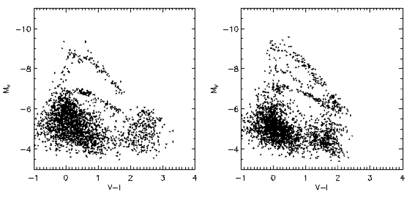
Figure 17: Simulated color-magnitude diagram for constant star formation rate in the range 4.0 – 100 Myr, using Geneva $Z=0.019$ (left) and $Z=0.008$ (right) isochrones.

While the 8 Myr isochrones show good agreement between Geneva and Padua models, significant differences exist for the older isochrones in the sense that the Geneva models produce cooler and fainter (in $V$-band) red supergiants for a given age. Another difference, which is not clearly seen from the isochrones but has important consequences for the CMD modeling, is that Geneva models spend more time as blue supergiants than the Padua models. Figure 17 shows constant-SFR simulated CMDs based on the Geneva isochrones. The left panel is for solar metallicity ($Z=0.020$) and the right panel is for $Z=0.008$. Compared to Fig. 11, the red supergiants are about 0.5 mag redder in $V\!-\!I$ for $Z=0.020$, while the $Z=0.008$ Geneva models produce RSGs of the about the same color as the Padua $Z=0.019$ models. Also note that Geneva models produce no RSGs brighter than $M_{V}=-6$ for solar metallicity, in better agreement with the observed CMD. The blue part of the CMD is actually dominated by blue supergiants older than about 15 Myr, rather than by very young main sequence stars.

When trying to reconstruct the observed CMD using the Geneva models, we found that no satisfactory fit could be obtained for the solar metallicity models, primarily because of the too red color of the RSGs. However, for the best-fitting solar metallicity models, two bursts were still preferred, with the youngest burst occurring at $\sim 6$ Myr and the older burst at 10–15 Myr. This difference in the age of the older burst compared to the Padua model fits is due to the fainter RSGs in the Geneva models at a given age. The $Z=0.008$ Geneva models produce a somewhat better fit to the observed CMD and the resulting SFH is very similar to the one based on the Padua models. A characteristic problem when using the Geneva models is that the large number of blue supergiants produced by populations older than about 15 Myr cannot easily be reconciled with the need for a very young population, because the blue part of the CMD tends to be too crowded below $M_{V}\approx-6$ in the presence of both.

Color-magnitude diagrams for other nearby galaxies do show some red supergiant stars in the magnitude interval predicted by the models for ages of 10–20 Myr, i.e. in the range $-8<M_{V}<-5$ (Wilson, Madore, & Freedman, 1990; Lynds et al., 1998; Cole et al., 1999). However, most of these CMDs are for lower-metallicity environments and thus may not be directly comparable to the situation in NGC 6946. Massey (1998) finds a steady decrease in the luminosity of the brightest red supergiants for selected fields in NGC 6822, M33 and M31 as a function of metallicity, with the brightest RSGs in M31 having $M_{V}\approx-6$. This is only slightly brighter than the brightest RSGs in the NGC 6946 complex.

Another shortcoming in our modeling is that we do not treat binary stars. For equal-mass binaries this would effectively make the integrated magnitudes brighter by 0.75 mag, while the situation is more complicated if the components have different masses. However, there is no conceivable way in which binaries could account for the “missing” red supergiants, except perhaps for their impact on stellar evolution in close systems.

3.4 Cluster ages revisited

Although the reddening presumably varies substantially at any given position within the complex, the reddening map (Fig. 6) provides some help in breaking the age-reddening degeneracy for stellar clusters. We thus return to the problem of determining cluster ages, now taking advantage of the improved knowledge about reddening. Table 3 lists data for each of the 18 clusters. Internal $A_{B}$ values from the reddening map are listed in the second column of the table, and the last two columns give the S-sequence ages derived from $UBV$ colors uncorrected and corrected for internal reddening, respectively. The reddening correction does affect the ages somewhat, but not dramatically. Girardi et al. (1995) quote an internal scatter of 0.14 in the S-sequence ages. In addition to this, photometric errors typically contribute with 0.2 to 0.4 in the uncertainty on log(age). Also, many of the same uncertainties concerning the evolution of massive stars dicussed in Section 3.3.4 affect estimates of cluster ages from their integrated colors.

A histogram of the cluster ages in the last column of Table 3 is shown in Figure 18. Note that the YSSC (age = 15 Myr) is not included in this plot. Like the SFH plots based on individual stars in Fig. 13, Figure 18 hints at two episodes of cluster formation, with a quiescent period around $\sim$15–25 Myr. Formally, the age distribution of the youngest clusters appears to peak earlier than the onset of the youngest burst of field star formation, but considering the uncertainties in the age determinations for clusters as well as stars it is not clear that this difference is significant. Also, the relative numbers of clusters of different ages are not easily comparable. Between an age of 6 Myr and 20 Myr a stellar cluster fades by $\approx 1.5$ mag in $V$ (Bruzual & Charlot, 2001), introducing a strong bias towards the youngest objects in a luminosity-limited sample, and dynamical destruction processes further reduce the number of clusters observed after $\sim 20$ Myr. Thus, it is quite likely that cluster formation took place throughout the star forming history of the complex, but most of the older clusters have faded beyond our detection limit or dissolved by now. Also note that the two oldest clusters, #99 and #2848, are located outside the main body of the complex and may be unrelated field objects.

4 Discussion

How does the complex in NGC 6946 compare with other large-scale star forming structures? In our Galaxy, the Sun itself is situated within a large structure, known as the Gould belt. The Gould belt has an estimated diameter of about 600–1000 pc, very similar to that of the complex in NGC 6946. The mean age is about 30 Myr, but with a large age spread (Stothers & Frogel, 1974; Poppel, 1997). From our vantage point within the Gould belt it is difficult to measure its total mass, but estimates range between $5\times 10^{4}$ M_⊙ (Comerón, Torra, & Gomez, 1994) and $5\times 10^{5}$ M_⊙ (Taylor, Dickman, & Scoville, 1987). Comerón (2001) quotes a total integrated $B$ magnitude of $M_{B}\approx-12.7$ for the Gould Belt. From our F439W images we get an integrated magnitude of $M_{B}=-15.1$ for the NGC 6946 complex (Table 2), i.e. about a factor of 10 brighter than the Gould Belt. Alternatively, our crude estimate of the total stellar mass (Section 3) of $\sim 10^{7}\mbox{${\rm M}_{\odot}$}$ is between 20 and 200 times higher than the above estimates for the Gould belt. The total ages are not well known for either the Gould belt or the NGC 6946 complex, but adopting characteristic ages of 30 Myr and 15 Myr, respectively, the mean SFR in the NGC 6946 complex appears to have been some 20 – 400 times higher than in the Gould belt.

Isolated arc-shaped or arc-including stellar complexes have been noted in a number of other galaxies (Efremov, 2001a), but detailed information about ages, masses and integrated luminosities is generally lacking. As the highest level in the hierarchy of clustering of young stellar populations, stellar complexes are omnipresent (Efremov, 1995; Elmegreen et al., 2000), but isolated complexes similar to the one investigated here are rare. For a complex in M83, Comerón (2001) estimated $M_{B}=-11.4$, a diameter of 450 pc and an age of $\sim 10^{7}$ years. Thus, the M83 complex is quite comparable in total luminosity and linear extent to the Gould belt, but about 30 times fainter than the complex in NGC 6946. Since it is probably also somewhat younger and therefore has a lower mass-to-light ratio, the mass difference may be even greater. The Quadrant arc in the LMC has an estimated mass of $3\times 10^{5}$ ${\rm M}_{\odot}$ (Efremov & Elmegreen, 1998) and the entire Constellation III may have a mass of some $10^{6}$ ${\rm M}_{\odot}$, again about an order of magnitude less than the NGC 6946 complex.

From this comparison, it is clear that the NGC 6946 complex presents a quite unique case, even just by its high concentration of very young stars and clusters. Other peculiar features include the luminous young super-star-cluster and the sharp western rim. Ideally, all these peculiar features should be explained jointly, possibly by some unusual process of star and cluster formation.

4.1 The intrinsic shape of the complex

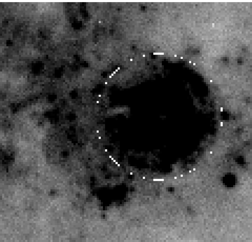
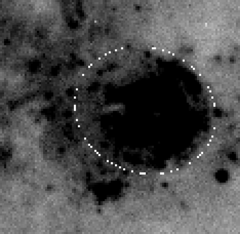
Figure 19: A NOT image of the complex, with circles and ellipses overlaid. North is up and east to the left in this figure.

The complex has a very sharp and regular outer rim, especially towards the west. The only other known features of such shape are the Quadrant (with the same radius, $\sim 300$ pc, and age, $\sim 15$ Myr) and Sextant arcs in the LMC (Efremov & Elmegreen, 1998). But what is the true 3-dimensional shape of the complex? Figure 19 shows NOT images displayed at high contrast to make the boundary between the complex and its surroundings more clear. The ellipse corresponds to a circular, but planar feature in the inclined disk of NGC 6946. Overall, the outer boundary of the complex appears to be better fitted by the circle than by the ellipse, suggesting a spherical rather than ring-like geometry (Efremov 2000; 2001), but note that only the western boundary is sharply defined. Towards the east the complex merges with the spiral arm and south of it are a number of young star forming regions embedded in H$\alpha$ emission, one of which (at the south-east) has an arc-like shape that is unlikely to be an artifact of light absorption, and was sketched by Hodge (1967). The W boundary of the complex by itself does not provide strong constraints in favor of either a circular or elliptical projected shape.

Of course, inferences about the 3D shape of the complex based on its 2D appearence rely heavily upon the assumption of either spherical or ring-like symmetry. It is difficult to imagine how a spherical complex with a diameter of about 600 pc could form in a presumably much thinner disk. A similar problem exists in the LMC for the Quadrant and Sextant arcs which also have have circular projected shapes, but larger radii than the thickness of the LMC gas disk (Efremov 2001a). The scale height of the Milky Way thin stellar disk is only about 100 pc (Gilmore, 1989) and the FWHM thickness of the molecular gas disk is $\approx 140$ pc (e.g. Bronfman et al., 1988). A thickness of 220 pc has been found for the molecular gas disk in the edge-on spiral NGC 891 (Scoville et al., 1993). The nearly face-on orientation of NGC 6946 makes it difficult to obtain information about the thickness of its disk, but Ehle & Beck (1993) presented a consistent model for Faraday rotation, depolarization and thermal radio emission in which most of the ionized gas in NGC 6946 resides in clouds within a disk of $\sim 100$ pc full thickness. Thus, it appears likely that the disk of NGC 6946 has a thickness of 100–200 pc and that much of the material in the complex is contained within about this height, implying a somewhat oblate intrinsic shape.

4.2 Origin

Our result that the complex has experienced two major star formation episodes clearly depends on the reliability of the stellar isochrones. However, multiple episodes of star formation separated by a few Myr are also known in other nearby starbursts such as 30 Dor (Rubio et al., 1998; Selman et al., 1999; Walborn et al., 1999), although on smaller scales, and might be a result of feedback mechanisms such as supernova explosions and winds from massive stars. While the Trewhella (1998) map shows less extinction in the Hodge complex compared to the surroundings, presumably indicating that the complex forms a cavity cleared out by stellar winds and supernovae over the past 25–30 Myr or more, we still see clear indications of substantial reddening variations across the complex, ranging from essentially no reddening to a $B$-band absorption of 1–2 mag or more. The regions of highest absorption are along the outer arc and near the two dark clouds identified in Paper I. In some of the denser parts of these clouds, star formation could still be taking place. In the following we briefly discuss a few possible scenarios for the formation of the complex, but we refer to Paper I and Efremov et al. (2001) for further details.

4.2.1 Formation by collapse of spiral arm gas

In Paper I it was shown that supernova explosions within the complex could have provided enough energy to clear out any residual gas and create the current bubble-like appearance. However, a more puzzling question is how such a large-scale star forming event was initiated in the first place at a relatively isolated location within NGC 6946. The location at the end of a spiral arm may be a clue to this question, and in Paper I it was suggested that the complex originated in a large-scale asymmetric collapse of gas at the end of the spiral arm. If the overall star formation efficiency was $\approx 10$% (typical for star formation in galactic Giant Molecular Clouds) then the initial gas mass must have been around $10^{8}$ ${\rm M}_{\odot}$. For a spherical cloud with a radius of 300 pc this corresponds to a mean density of $n(H_{2})\approx 20\,{\rm cm}^{-3}$, or higher for a flattened geometry. Thus, the proto-cloud may have resembled the “Super Giant Molecular Clouds” proposed by Harris & Pudritz (1994) as the progenitors of globular clusters. Fig. 1 in Paper I shows regions of star formation at similar positions with respect to other spiral arms in NGC 6946, although none of them have quite as striking an appearance as the complex discussed here. However, most of these other regions are still dominated by H$\alpha$ emission, indicating younger ages than for the Hodge complex. The peculiar appearance of the latter may be related to the clearing of gas, providing a better view of its stellar contents.

The high density of the YSSC is not surprising considering the environment in which it was born. The star formation history in this region suggests that 15 Myr ago there was a bright association of stars with a total mass of around $4\times 10^{6}$ M_⊙, from the integral under the curve of the oldest burst in Figure 13. This mass corresponds to an enormous luminosity and energy output in the form of HII regions, stellar winds and supernovae, but it is not unusual compared to other giant star complexes in the outer spiral arms of galaxies. For example, the supergiant HII regions in the study by Kennicutt (1984) contain over 1000 OB stars; considering the IMF, this corresponds to over $10^{6}$ M_⊙ of total stars. The stellar energy from the association in NGC 6946 would have immediately begun to clear a cavity around it, eventually leading to the big bubble seen today. At the same time, it would have compressed any residual molecular material and triggered more star formation. Because the formation of an OB association is relatively inefficient, there was probably a few times $10^{7}$ M_⊙ of dense gas left over within 100 pc or so of the first generation stars. If about $10^{7}$ M_⊙ of this residual material was in the form of one large cloud, then the compressed part of this cloud facing the association core would have made one large and dense cluster, which is now the YSSC. A similar phenomenon, scaled down by a factor of $\sim 100$, occurred in the Orion association, with the Trapezium cluster triggered in the comet-shaped head of a GMC (Bally et al., 1987) compressed by the older Orion association. The triggered stars in NGC 6946 formed with an equally high efficiency as the Trapezium cluster, leaving a bound remnant, and then broke apart its remaining GMC into the two pieces that are now seen as two dark clouds, one to the North and the other to the East of the YSSC. A faint arc of extinction connects these two clouds giving the impression of a partial shell centered on the YSSC. At this time, the combined pressures from the aging first generation of stars, which is getting more and more dispersed with time, and the YSSC drove the expansion of the bubble further and triggered more star formation. This third generation of stars had a more distributed pattern than the YSSC, forming a lot of smaller clusters, because the clouds were more dispersed when they formed. It is evident as the young burst in figure 13. One feature which remains unexplained in this scenario is the sharp western rim; however, it is not clear to what extent this is real or an effect of dust obscuration.

4.2.2 High velocity cloud impact

Another mechanism which might explain the formation of the complex is the infall of a massive high velocity cloud. Some support for this idea is provided by the fact that NGC 6946 is known to have a large number of such clouds projected on its disk (Boulanger & Viallefond, 1992; Kamphuis, 1993). The velocity of the YSSC and of the HII gas inside and near the complex being on average the same and quite similar to the rotational velocity of the galaxy at this position (Efremov et al., 2001), one has to conclude that the infall was oblique, i.e. the trajectory of the infalling cloud had a small angle to the galaxy plane. Note also that the Eastern edge of the complex is neither sharp nor circular and the overall shape of the complex resembles a comet with a very short Eastward tail (see Figure 7 in Paper I). The shape of the complex in comparison with simulations of partial spheres seen under different angles indicates an infall angle of about 10–20 degrees or so (Efremov, 2001a, b). This suggestion seems to be compatible with the comet-like shape of the complex, which may indicate a Westward movement of the impacting cloud. The radial velocity of the YSSC and the bulk of the surrounding ionized gas is about 150 km/s (Larsen et al., 2001; Efremov et al., 2001), whereas the average rotational velocity of surrounding HII gas is about 130 km/sec. This is compatible with the infall hypothesis. We note that the infall of a high-velocity cloud has also been suggested as the formation mechanism for the Gould belt (Comerón, Torra, & Gomez, 1994).

4.2.3 Super-explosions

Finally, we consider the possibility originally suggested by Hodge (1967), namely a highly energetic explosion, which might have triggered star formation in shells of swept-up gas and generated the arc-like structures. Some support for this idea is found in data on the kinematics of HII gas in the complex, which display two young expanding HII shells with different expansion velocities and dynamical ages of a few Myr (Efremov et al., 2001). Formation of some of the younger stars might have been triggered by hypernova progenitors ejected from the YSSC (Efremov, 2001a), although the formation of the older stellar population in the complex and the YSSC itself is not easily explained as due to such super-explosions.

4.2.4 The young super star cluster

Noting the high density of point sources near the YSSC, it was suggested in Paper I that the YSSC might have formed from accretion of a number of less luminous clusters surrounding it. Fig. 2 shows 4 clusters (#865, #975, #1094 and #1236) near the YSSC, but it is now clear that many of the luminous objects near the YSSC are probably not clusters, but individual $\lesssim 6$ Myr old stars. Thus, the case for formation of the YSSC by coalescence of smaller clusters may have been weakened. The cluster may simply have formed by normal star formation mechanisms, albeit on a much larger scale than is seen in the Milky Way.

In addition to the $A_{B}=1.48$ foreground absorption, the reddening map indicates an internal absorption of $A_{B}=0.53$ at the position of the YSSC, or $A_{B}$(total) = 2.01 mag. Alternatively, the $Q$-method (van den Bergh & Hagen, 1968) gives an internal absorption of $A_{B}=1.04$, or $A_{B}$(total) = 2.52. The cluster might therefore be as bright as $M_{V}\approx-14$.

Although the YSSC has an unusually high luminosity (and mass) for a young star cluster in a normal spiral galaxy, other similarly luminous clusters are known elsewhere. Similar bright clusters exist in galaxies such as M51, M83 and NGC2997 (Larsen & Richtler, 1999; Larsen, 2000), some of which are nearly as bright as the YSSC in NGC 6946, and the 2nd brightest cluster within NGC 6946 is only about 1 magnitude fainter than the YSSC. The cluster is also quite comparable to the most luminous clusters in starburst galaxies (e.g. Whitmore, 2001). Characteristic for all these bright clusters is that they are found in environments of high star formation activity.

It is interesting to consider how the complex fits into the SFR vs. specific cluster luminosity relation discussed by Larsen & Richtler (2000). From the photometry in Table 2 and Paper II we obtain the specific $U$-band luminosity $T_{L}(U)$ for the YSSC with respect to the complex as

$$T_{L}(U)=100\,L_{\rm YSSC}/L_{\rm complex}=18$$ (2)

This is among the highest $T_{L}(U)$ values seen anywhere. Again, internal reddening has not been taken into account, but since this should affect both the cluster and the complex we have simply chosen to use the directly observed luminosities. Actually, since the colors of the YSSC and the complex as a whole are very similar, it doesn’t matter much in which band the specific luminosity is computed in this particular case. For a total complex mass of $10^{7}$ ${\rm M}_{\odot}$, radius 0.3 kpc and age 15 Myr, the star formation rate surface density $\Sigma_{\rm SFR}$ = 2.4 ${\rm M}_{\odot}$ yr^-1 kpc^-2, even higher than any galaxy studied by Larsen & Richtler (2000). It should be noted that they defined $T_{L}(U)$ for a cluster system with respect to the integrated luminosity of the entire underlying galaxy, which includes some contribution from older stellar populations even in $U$. It is also not obvious that the same $\Sigma_{\rm SFR}$– $T_{L}(U)$ relation observed for galaxies is valid locally.

Nevertheless, the problem of understanding the presence of the YSSC in the NGC 6946 complex is perhaps no different from understanding the presence of massive star clusters in actively star forming environments in general. With an initial gas supply of some $10^{8}$ ${\rm M}_{\odot}$ within a radius of 300 pc, collecting $\sim 10^{6}$ ${\rm M}_{\odot}$ in a dense core and forming a massive cluster there does not seem difficult. The fact that such massive clusters are not observed in the Gould belt might simply be due to the much lower star formation density there.

5 Summary and Conclusions

We have presented HST WFPC2 data for a peculiar stellar complex in NGC 6946. The complex is dominated by a young super star cluster which accounts for about 18% of the total luminosity of the complex. The linear dimensions are similar to those of the local Gould belt, but the total stellar mass contained within the NGC 6946 complex is 1 – 2 orders of magnitude higher. The complex thus has the characteristics of a (very localized) starburst, which might explain the presence of a very luminous cluster within it. The cluster itself presumably formed in the same way as massive clusters elsewhere, in the dense core of a large concentration of molecular gas. In addition the the YSSC, the complex also contains a number of clusters with more modest luminosities; however, about a dozen of these are still comparable to the brightest young clusters in the Milky Way.

We have demonstrated that it is possible to model the CMD of stars in the complex by a superposition of currently available stellar isochrones. The best match is obtained for solar-metallicity models from the Padua group. From the CMD modeling we have found tentative evidence for two star forming episodes within the complex. The time of onset for the first burst is not well constrained in our data but may have occurred some 25–30 Myr or longer ago. This burst lasted until 15–20 Myr ago and was followed first by the formation of the YSSC, and then by a quiescent period. The second burst began about 6 Myr ago and may be continuing until the present day. However, the apparent age gap relies on the model prediction that a 10–20 Myr old population should produce a substantial number of red supergiants brighter than $M_{V}=-5$, which are not observed. If no RSGs are produced in this age range, or if they are fainter than predicted, then an age gap might not be required. Stars in the corresponding mass range, 12 – 18 M_⊙, are not usually believed to become Wolf-Rayet stars (Maeder & Conti, 1994), although it has been suggested that stars in M31 with masses as low as 13 – 15 M_⊙ might become W-R stars, spending at most only a brief period as RSGs (Massey, 1998). Clearly, a more detailed analysis has to await a better understanding of the evolution of massive stars, but in the meantime the NGC 6946 complex might serve as another testbed for such studies. Some support for two episodes of star formation is also seen in the age distribution of stellar clusters.

The circumstances leading to the formation of the complex remain elusive, but we have briefly discussed a few possible scenarios: 1) Collapse of a large concentration of spiral arm gas, as suggested by Elmegreen, Efremov & Larsen (2000). This initially formed a $4\times 10^{6}$ M_⊙ OB association, which subsequently compressed any residual gas and triggered further star formation, including the YSSC; 2) impact by a high-velocity cloud, suggested as the formation mechanism for the Gould belt (Comerón, Torra, & Gomez, 1994); 3) Shock compression of a gas cloud by an energetic super-explosion, following the suggestion by Hodge (1967).

The best way to make further progess in the understanding of this peculiar stellar complex would be high resolution HI and CO data. The gas distributions and velocities might still have imprints of the event which formed the complex. Existing data for the gas show no peculiarities, except for two expanding young HII supershells (Efremov et al. 2001), which are probably connected with the younger stellar generation. Imaging at near-infrared wavelengths would also help in penetrating through regions of high extinction, providing a clearer view of the true morphology of the complex.

Figure 1: A color composite image showing the complex centered on the PC chip. The image is an approximation to a true-color image and was assembled from F336W and F439W (blue), F555W (green) and F555W, F814W and F656N (red). HII regions appear red.

Figure 2: An F555W ($V$-band) image of the stellar complex showing the location of cluster candidates, i.e. objects with $M_{V}<-7.5$ and FWHM$>\mbox{$0.4$}$ pixels. The arrow indicates the North and East directions.

Figure 4: ($(\bv)_{0}$, $(\ub)_{0}$) two-color diagram for objects brighter than $V=22.5$ ($M_{V}=-7.5$) (aperture photometry), corrected for foreground reddening. Point sources (FWHM$<$$0.4$ pixels) are shown with diamond symbols. The solid line is the Girardi et al. (1995) “S”-sequence, while two isochrones from Girardi et al. (2000) (4 and 10.0 Myr) are shown with dashed lines. The arrow indicates the reddening vector corresponding to $E(B-V)=0.5$ mag.

Figure 5: Evolution of the reddening-free $Q_{1}$ index as a function of age for $Z=0.02$ (solar), $Z=0.008$ and $Z=0.004$.

Figure 6: Reddening map with red and blue indicating high and low reddening, respectively. The wedge at the bottom indicates a range from $A_{B}=1.5$ to $A_{B}=3.5$. Individual reddenings were determined from the $UBV$ colors of stars and the map was produced by smoothing with an Epanechnikov kernel.

Figure 8: Spatial distributions of early-type stars stars brighter than $V=23.5$ ($M_{V}<-6.5$) (left) and red supergiants (right). The early-type (main sequence and supergiant) stars appear to be more concentrated towards the center of the complex.

Figure 13: Star formation history derived from CMD fitting for three different assumptions about internal extinction in the complex. The SFR has been normalized assuming a total complex mass of $10^{7}$ ${\rm M}_{\odot}$. The Gaussian curve represents the young super star cluster.

Figure 15: Star formation histories for the central 100 pixels and for $100<r<300$ pixels.

Figure 16: Comparison of solar-metallicity isochrones from the Padua group (Girardi et al., 2000) and Geneva group (Lejeune & Schaerer, 2001). The Geneva isochrones produce cooler and fainter red supergiants for a given age.

Figure 18: Histogram of cluster ages, determined from de-reddened $UBV$ colors and the Girardi et al. (1995) S-sequence calibration.

Table 1: Aperture Corrections, ($11\rightarrow 3$ pixels)

Filter	FWHM (pixels / pc)
	0 / 0	0.25 / 0.32	0.50 / 0.64	1.00 / 1.29
F336W	$-0.158$	$-0.295$	$-0.534$	$-0.849$
F439W	$-0.159$	$-0.296$	$-0.536$	$-0.853$
F555W	$-0.152$	$-0.304$	$-0.547$	$-0.867$
F814W	$-0.210$	$-0.370$	$-0.611$	$-0.923$

Note. — Aperture corrections (in magnitudes) are for the PC chip for objects with intrinsic FWHM values as listed. Note that the F336W, F439W and F555W aperture corrections are very similar, independently of object size.

Table 2: Data for the brightest clusters

Object	$x,y$	$M_{V}$	$(\ub)_{0}$	$(\bv)_{0}$	$(V\!-\!I)_{0}$	$Q_{1}$
Complex	400,400	$-15.0$	$-0.76$	$-0.05$	0.36	$-0.72$
YSSC	520,380	$-13.2$	$-0.72$	0.10	0.59	$-0.80$
99	103,112	$-7.99\pm 0.06$	$-0.41\pm 0.14$	$0.03\pm 0.09$	$0.25\pm 0.06$	$-0.44\pm 0.16$
502	563,259	$-8.65\pm 0.04$	$-0.62\pm 0.07$	$-0.05\pm 0.06$	$0.22\pm 0.04$	$-0.59\pm 0.09$
539	426,270	$-9.37\pm 0.03$	$-0.74\pm 0.08$	$0.11\pm 0.06$	$0.50\pm 0.04$	$-0.83\pm 0.09$
865	496,331	$-8.81\pm 0.04$	$-0.50\pm 0.14$	$0.05\pm 0.10$	$0.38\pm 0.07$	$-0.54\pm 0.16$
894	362,338	$-8.97\pm 0.03$	$-0.88\pm 0.11$	$-0.16\pm 0.10$	$0.63\pm 0.07$	$-0.77\pm 0.13$
975	492,349	$-8.76\pm 0.05$	$-0.44\pm 0.11$	$0.24\pm 0.07$	$0.58\pm 0.04$	$-0.62\pm 0.12$
1094	520,364	$-10.18\pm 0.02$	$-0.78\pm 0.04$	$-0.05\pm 0.04$	$0.51\pm 0.03$	$-0.75\pm 0.05$
1112	303,367	$-9.04\pm 0.03$	$-1.05\pm 0.06$	$-0.26\pm 0.06$	$-0.26\pm 0.05$	$-0.87\pm 0.08$
1236	472,382	$-9.04\pm 0.04$	$-0.34\pm 0.23$	$0.26\pm 0.12$	$0.72\pm 0.07$	$-0.54\pm 0.25$
1443	292,408	$-9.27\pm 0.03$	$-0.80\pm 0.06$	$-0.04\pm 0.05$	$0.43\pm 0.03$	$-0.78\pm 0.07$
1448	370,407	$-9.28\pm 0.03$	$-1.06\pm 0.14$	$0.26\pm 0.13$	$0.18\pm 0.09$	$-1.27\pm 0.18$
1499	302,415	$-9.37\pm 0.03$	$-0.93\pm 0.06$	$-0.15\pm 0.06$	$-0.31\pm 0.05$	$-0.83\pm 0.08$
1688	222,442	$-9.08\pm 0.03$	$-0.74\pm 0.09$	$0.08\pm 0.07$	$0.64\pm 0.04$	$-0.81\pm 0.10$
1805	435,459	$-10.31\pm 0.02$	$-0.82\pm 0.04$	$-0.01\pm 0.03$	$0.12\pm 0.02$	$-0.82\pm 0.04$
1950	257,479	$-9.23\pm 0.03$	$-0.39\pm 0.09$	$0.32\pm 0.06$	$0.96\pm 0.03$	$-0.64\pm 0.10$
2228	358,529	$-9.07\pm 0.03$	$-0.56\pm 0.12$	$-0.07\pm 0.08$	$0.52\pm 0.06$	$-0.51\pm 0.13$
2284	536,536	$-8.52\pm 0.04$	$-0.90\pm 0.09$	$-0.22\pm 0.08$	$-0.23\pm 0.07$	$-0.75\pm 0.10$
2848	389,758	$-8.78\pm 0.03$	$-0.39\pm 0.11$	$0.17\pm 0.07$	$0.53\pm 0.04$	$-0.52\pm 0.12$

Note. — $M_{V}$ values are measured in $r=11$ pixels (0$\farcs$5) aperture. Colors in $r=3$ aperture, with aperture corrections to $r=11$ pixels. Log(age) are from the S-sequence calibration. In addition to the intrinsic scatter of 0.14, typical uncertainties on log(age) are about 0.3.

Table 3: Cluster ages

Object	$A_{B}^{i}$	agenocorr (Myr)	agecorr (Myr)
99	0.00	61	61
502	0.53	31	27
539	0.46	12	10
865	0.81	42	35
894	0.93	12	8
975	0.70	38	33
1094	0.58	15	12
1112	0.58	4	3
1236	0.64	53	46
1443	0.59	13	10
1448	0.84	1	1
1499	0.61	8	6
1688	1.05	13	10
1805	0.52	11	9
1950	1.03	39	31
2228	0.87	41	33
2284	0.20	12	11
2848	0.00	51	51

Note. — $A_{B}^{i}$ is the internal reddening for the cluster, determined from the reddening map. age_nocorr and age_corr are the S-sequence ages in Myr without and with correction for internal reddening.

Table 4: Data for CMD fits

Field	$A_{B}$	$\chi^{2}$	$N$
All	0.0	4.4	2567
All	0.0–1.0	1.0	2567
All	0.0–2.0	3.6	2567
$0<r<100$ pixels	0.0–1.0	2.3	560
$0<r<100$ pixels	0.0–2.0	3.2	560
$100<r<300$ pixels	0.0–1.0	1.2	1539
$100<r<300$ pixels	0.0–2.0	1.6	1539
$0<r<100$ pixels	0.0–1.0	2.3	560
$100<r<150$ pixels	0.0–1.0	2.1	527
$150<r<200$ pixels	0.0–1.0	1.3	499
$200<r<250$ pixels	0.0–1.0	0.9	316

Note. — $N$ is the number of stars in the observed CMD

References

- Bally et al. (1987) Bally, J., Langer, W. D., Stark, A. A., & Wilson, R. W. 1987, ApJ, 312, L45
- Bertelli et al. (1992) Bertelli, G., Mateo, M., Chiosi, C., & Bressan, A. 1992, ApJ, 388, 400
- Bertelli et al. (1994) Bertelli, G., Bressan, A., Chiosi, C., Fagotto, F., & Nasi, E. 1994, A&AS, 106, 275
- Bianchi et al. (2000) Bianchi, S., Davies, J. I., Alton, P. B., Gerin, M., & Casoli, F. 2000, A&A, 353, L13
- Bonnarel et al. (1988) Bonnarel, F., Boulesteix, J., Georgelin, Y. P., Lecoarer, E., Marcelin, M., Bacon, R., & Monnet, G. 1988, A&A, 189, 59
- Boulanger & Viallefond (1992) Boulanger, F. & Viallefond, F. 1992, A&A, 266, 37
- Bronfman et al. (1988) Bronfman, L., Cohen, R. S., Alvarez, H., May, J., & Thaddeus, P. 1988, ApJ, 324, 248
- Bruzual & Charlot (2001) Bruzual, G. A. and Charlot, S. 2001, in preparation.
- Burstein & Heiles (1984) Burstein, D. & Heiles, C. 1984, ApJS, 54, 33
- Cardelli, Clayton & Mathis (1989) Cardelli, J. A., Clayton, G. C. and Mathis, J. S. 1989, ApJ, 345, 245
- Chiosi (1998) Chiosi, C. 1998, p. 1 in: “Stellar Astrophysics for the Local Group”, Cambridge Contemporary Astrophysics, eds. A. Aparicio, A. Herrero and F. Sánchez
- Cole et al. (1999) Cole, A. A. et al. 1999, AJ, 118, 1657
- Comerón, Torra, & Gomez (1994) Comeron, F., Torra, J., & Gomez, A. E. 1994, A&A, 286, 789
- Comerón (2001) Comerón, F. 2001, A&A, 365, 417
- Degioia-Eastwood et al. (1984) Degioia-Eastwood, K., Grasdalen, G. L., Strom, S. E., & Strom, K. M. 1984, ApJ, 278, 564
- Dirsch et al. (2000) Dirsch, B., Richtler, T., Gieren, W. P., & Hilker, M. 2000, A&A, 360, 133
- Dolphin (2000) Dolphin, A. E. 2000, MNRAS, 313, 281
- Eastman, Schmidt, & Kirshner (1996) Eastman, R. G., Schmidt, B. P., & Kirshner, R. 1996, ApJ, 466, 911
- Efremov (1995) Efremov, Y. N. 1995, AJ, 110, 2757
- Efremov & Elmegreen (1998) Efremov, Y. N. & Elmegreen, B. G. 1999, MNRAS, 299, 643
- Efremov (2001a) Efremov, Y. N. 2001a, Astron. Rep. 45, 769
- Efremov (2001b) Efremov, Y. N. 2001b, In: Extragalactic star clusters, IAU Symp. Ser., Vol. 207, eds. E.K.Grebel, D.Geisler and D.Minniti,
- Efremov et al. (2001) Efremov, Y. N., Pustilnik, S. A., Kniazev, A. Y., et al. 2001, A&A, submitted
- Ehle & Beck (1993) Ehle, M. & Beck, R. 1993, A&A, 273, 45
- Elmegreen (2000) Elmegreen, B. G. 2000, ApJ, 530, 277
- Elmegreen et al. (2000) Elmegreen, B. G., Efremov, Y., Pudritz, R. E., & Zinnecker, H. 2000, Protostars and Planets IV, 179
- Elmegreen & Efremov (1997) Elmegreen, B. G. & Efremov, Y. N. 1997, ApJ, 480, 235
- Elmegreen, Efremov & Larsen (2000) Elmegreen, B. G., Efremov, Yu. N., & Larsen, S. S. 2000, ApJ, 535, 748 (Paper I)
- Elmegreen, Chromey, & Santos (1998) Elmegreen, D. M., Chromey, F. R., & Santos, M. 1998, AJ, 116, 1221
- Engelbracht et al. (1996) Engelbracht, C. W., Rieke, M. J., Rieke, G. H., & Latter, W. B. 1996, ApJ, 467, 227
- Ferguson, Gallagher, & Wyse (1998) Ferguson, A. M. N., Gallagher, J. S., & Wyse, R. F. G. 1998, AJ, 116, 673
- Gallart et al. (1999) Gallart, C., Freedman, W. L., Aparicio, A., Bertelli, G., & Chiosi, C. 1999, AJ, 118, 2245
- Gilmore (1989) Gilmore, G. 1989, p. 9, in: “The Milky Way as a Galaxy”, Saas-Fee Advanced Course No. 19, University Science Books, eds. R. Buser and I. R. King
- Girardi et al. (1995) Girardi, L., Chiosi, C., Bertelli, G., Bressan, A. 1995, A&A, 298, 87
- Girardi et al. (2000) Girardi, L., Bressan, A., Bertelli G., Chiosi C. 2000, A&AS, 141, 371
- Gray & Toner (1987) Gray, D. F. & Toner, C. G. 1987, ApJ, 322, 360
- Harris & Zaritsky (2001) Harris, J. and Zaritsky, D. 2001, ApJ Suppl. in press (astro-ph/0104202)
- Harris & Pudritz (1994) Harris, W. E. & Pudritz, R. E. 1994, ApJ, 429, 177
- Harris, Zaritsky, & Thompson (1997) Harris, J., Zaritsky, D., & Thompson, I. 1997, AJ, 114, 1933
- Hodge (1967) Hodge, P. W. 1967, PASP, 79, 29
- Holtzman et al. (1995) Holtzman, J. A., Burrows, C. J., Casertano, S., et al. 1995, PASP, 107, 1065
- Holtzman et al. (1999) Holtzman, J. A. et al. 1999, AJ, 118, 2262
- Humphreys (1980) Humphreys, R. M. 1980, ApJ, 241, 587
- Kamphuis (1993) Kamphuis, J. J. 1993, PhD thesis, University of Groningen
- Karachentsev, Sharina & Huchtmeier (2000) Karachentsev, I. D., Sharina, M. E. & Huchtmeier, W. K. 2000, A&A, 362, 544
- Kennicutt (1984) Kennicutt, R. C. 1984, ApJ, 287, 116
- Krist & Hook (1997) Krist, J., & Hook, R. 1997, “The Tiny Tim User’s Guide”, STScI
- Larsen (1999) Larsen, S. S. 1999, A&AS, 139, 393
- Larsen (2000) Larsen, S. S. 2000, MNRAS, 319, 893
- Larsen, Forbes & Brodie (2001) Larsen, S. S., Forbes, D. A., & Brodie, J. P. 2001, MNRAS, 327, 1116
- Larsen & Richtler (1999) Larsen, S. S. & Richtler, T. 1999, A&A, 345, 59
- Larsen & Richtler (2000) Larsen, S. S. & Richtler, T. 2000, A&A, 354, 836
- Larsen et al. (2001) Larsen, S. S., Brodie, J. P., Elmegreen, B. G., Efremov, Y. N., Hodge, P. W., Richtler, T. 2001, ApJ, 556, 801 (Paper II)
- Lejeune & Schaerer (2001) Lejeune, T. & Schaerer, D. 2001, A&A, 366, 538
- Lynds et al. (1998) Lynds, R., Tolstoy, E., O’Neil., E. J., & Hunter, D. A. 1998, AJ, 116, 146
- Maeder & Conti (1994) Maeder, A. ; & Conti, P. S. 1994, ARA&A, 32, 227
- Maeder & Meynet (2000) Maeder, A. ; & Meynet, G. 2000, ARA&A, 38, 143
- Malhotra et al. (1996) Malhotra, S. et al. 1996, A&A, 315, L161
- Massey (1998) Massey, P. 1998, ApJ, 501, 153
- McCall, Rybski, & Shields (1985) McCall, M. L., Rybski, P. M., & Shields, G. A. 1985, ApJS, 57, 1
- Olsen (1999) Olsen, K. A. G. 1999, AJ, 117, 2244
- Poppel (1997) Poppel, W. 1997, Fundamentals of Cosmic Physics, 18, 1
- Press et al. (1992) Press, W. H., Teukolsky, S. A., Vetterling, W. T., Flannery, B. P., 1992 Numerical Recipes in C/Fortran, Cambridge University Press
- Ratnatunga & Bahcall (1985) Ratnatunga, K. U. & Bahcall, J. N. 1985, ApJS, 59, 63
- Rubio et al. (1998) Rubio, M., Barbá, R. H., Walborn, N. R., Probst, R. G., García, J., & Roth, M. R. 1998, AJ, 116, 1708
- Salasnich, Bressan, & Chiosi (1999) Salasnich, B., Bressan, A., & Chiosi, C. 1999, A&A, 342, 131
- Salpeter (1955) Salpeter, E. E. 1955, ApJ, 121, 161
- Sauty, Gerin, & Casoli (1998) Sauty, S., Gerin, M., & Casoli, F. 1998, A&A, 339, 19
- Schlegel (1994) Schlegel, E. M. 1994, AJ, 108, 1893
- Schlegel et al. (1998) Schlegel, D. J., Finkbeiner, D. P., & Davis, M. 1998, ApJ, 500, 525
- Schlegel, Blair, & Fesen (2000) Schlegel, E. M., Blair, W. P., & Fesen, R. A. 2000, AJ, 120, 791
- Scoville et al. (1993) Scoville, N. Z., Thakkar, D., 1993, ApJ, 404, L59
- Selman et al. (1999) Selman, F., Melnick, J., Bosch, G., & Terlevich, R. 1999, A&A, 347, 532
- Shklovsky (1960) Shklovsky, I. S. 1960, Soviet Astron. AJ, 4, 35
- Stetson (1987) Steton, P. B. 1987, PASP, 99, 191
- Stothers & Frogel (1974) Stothers, R. & Frogel, J. A. 1974, AJ, 79, 456
- Tacconi & Young (1989) Tacconi, L. J. & Young, J. S. 1989, ApJS, 71, 455
- Taylor, Dickman, & Scoville (1987) Taylor, D. K., Dickman, R. L., & Scoville, N. Z. 1987, ApJ, 315, 104
- Trewhella (1998) Trewhella, M. 1998, MNRAS, 297, 807
- Tully (1988) Tully, B. 1988, Nearby Galaxies Catalog, Cambridge University Press
- van den Bergh & Hagen (1968) van den Bergh, S. & Hagen, G. L. 1968, AJ, 73, 569
- Walborn et al. (1999) Walborn, N. R., Barbá, R. H., Brandner, W., Rubio, M. ;., Grebel, E. K., & Probst, R. G. 1999, AJ, 117, 225
- Whitmore (2001) Whitmore, B. C. 2001, astro-ph/0012546
- Wilson, Madore, & Freedman (1990) Wilson, C. D., Madore, B. F., & Freedman, W. L. 1990, AJ, 99, 149
- Wyder (2001) Wyder, T. K. 2001, BAAS, 197, 2803