The X-ray surface brightness profiles of hot galaxy clusters up to $z\sim 0.8$: evidence for self-similarity and constraints on $\rm\Omega_{0}$

We study the surface brightness profiles of a sample of 25 distant $(0.3<z<0.83)$ hot $({\rm k}T>3.5\leavevmode\nobreak\ \rm keV)$ clusters, observed with ROSAT, with published temperatures from ASCA. For both open and flat cosmological models, the derived emission measure profiles are scaled according to the self-similar model of cluster formation. We use the standard scaling relations of cluster properties with redshift and temperature, with the empirical slope of the $M_{\rm gas}$–$T$ relation derived by Neumann & Arnaud (neumann01 (2001)). Using a $\chi^{2}$ test, we perform a quantitative comparison of the scaled emission measure profiles of distant clusters with a local reference profile derived from the sample of 15 hot nearby clusters compiled by Neumann & Arnaud (1999), which were found to obey self-similarity. This comparison allows us to both check the validity of the self-similar model across the redshift range $0.04-0.8$, and to constrain the cosmological parameters.
For a low density flat universe, the scaled distant cluster data were found to be consistent, both in shape and normalisation, with the local reference profile. It indicates that hot clusters constitute a homologous family up to high redshifts, and gives support to the standard picture of structure formation for the dark matter component. Because of the intrinsic regularity in the hot cluster population, the scaled profiles can be used as distance indicators, the correct cosmology being the one for which the various profiles at different redshifts coincide. The intrinsic limitations of the method, in particular possible systematic errors and biases related to the model uncertainties, are discussed. Using the standard evolution model, the present data allow us to put a tight constraint on $\rm\Omega_{0}$ for a flat Universe: $\rm\Omega_{0}=0.40^{+0.15}_{-0.12}$ at 90% confidence level (statistical errors only). The critical model ($\rm\Omega_{0}=1$) was excluded at the 98% confidence level. Consistently, the observed evolution of the normalisation of the $L_{\rm X}$–$T$ relation was found to comply with the self-similar model for $\rm\Omega_{0}=0.4$, $\Lambda=0.6$. The constraint derived on $\rm\Omega_{0}$ is in remarkable agreement with the constraint obtained from luminosity distances to SNI or from combined analysis of the power spectrum of the 2dF galaxy redshift Survey and the Cosmic Microwave Background anisotropies.

1 Introduction

In the simplest models of structure formation, purely based on gravitation, galaxy clusters constitute a homologous family. Clusters are self-similar in shape, and predictable scaling laws relate each physical property to the cluster total mass $M$ and redshift $z$ (Kaiser kaiser86 (1986); Navarro et al. navarro97 (1997); Teyssier et al. teyssier (1997); Eke et al. eke (1998); Bryan & Norman bryan98 (1998)). Self-similarity applies to both the dark matter component and the hot X–ray emitting intra-cluster medium (ICM).

From the observation of the ICM, we do see regularity in the local ($z<0.1$) population of clusters, like strong correlations between luminosity, gas mass, total mass, size and temperature $T$ (Mohr et al. mohr97 (1997); Allen & Fabian allen (1998); Markevitch markevitch (1998); Arnaud & Evrard arnaud (1999); Horner et al. horner (1999); Mohr et al. mohr99 (1999);Vikhlinin, et al. vikhlinin99 (1999); Nevalainen et al. nevalainen (2000); Finoguenov et al. finoguenov (2001); Xu et al. xu (2001)). Furthermore, there is strong indication of a universal shape for the density and temperature profiles of hot (${\rm k}T>4\leavevmode\nobreak\ \rm keV$) clusters, beyond the cooling flow region (Markevitch et al. markevitch98 (1998); Neumann & Arnaud neumann99 (1999), neumann01 (2001); Vikhlinin, et al. vikhlinin99 (1999); Irwin & Bregman irwin (2000); Arnaud arnaud01 (2001)). However, clusters also deviate from the simplest self-similar model. The most remarkable deviation is the slope of the luminosity–temperature ($L_{\rm X}$–$T$ ) relation, which is steeper than predicted. In a recent study, Neumann & Arnaud (neumann01 (2001)) showed that a steepening of the $M_{\rm gas}$–$T$ relation ($M_{\rm gas}\propto T^{1.94}$, instead of the standard relation $M_{\rm gas}\propto T^{1.5}$) can explain the observed $L_{\rm X}$–$T$ relation in the hot temperature domain, and account for the scaling properties of the normalisation of the emission measure profiles of hot clusters. Similar steepening was derived from direct studies of the $M_{\rm gas}$–$T$ relation independently carried out (Mohr et al. mohr99 (1999); Vikhlinin, et al. vikhlinin99 (1999)) and is also consistent with the observed slope of the isophotal size–temperature ($S_{\rm I}$–$T$ ) relation (Mohr et al. mohr97 (1997)).

Several physical processes have been suggested to explain the departure from the simplest self-similar model. Pre-heating by early galactic winds, has been proposed to explain the steepening of the $L_{\rm X}$–$T$ relation (e.g. Kaiser kaiser91 (1991); Evrard & Henry evrard91 (1991)), although other effects like AGN heating (e.g. Valageas & Silk valageas (1999); Wu et al.  wu (2000)), radiative cooling (Pearce et al.  pearce (2000); Muawong et al. muawong (2001)) or variation of the galaxy formation efficiency with system mass (Bryan bryan00 (1998)) might also play a role. Further evidence of the importance of non-gravitational processes is provided by the excess of entropy (the “entropy floor”) in poor clusters (Ponman et al. ponman (1999); Lloyd-Davis et al. lloyd (2000)). Recent numerical simulations (Bialek et al. bialek (1999)) including pre-heating, with an initial entropy level consistent with this observed entropy floor, do predict a steepening of the $L_{\rm X}$–$T$ , $M_{\rm gas}$–$T$ and $S_{\rm I}$–$T$ relations, consistent with the observations quoted above (see also Loewenstein loewenstein (2000); Tozzi & Norman tozzi (2001); Brighenti & Mathews brighenti (2001); Borgani et al.  borgani (2001)). However, it is unclear if such a scenario is also consistent with the level of self-similarity in shape observed in hot clusters. Although it is predicted that cool clusters should have a more extended atmosphere than hot clusters (e.g. Tozzi & Norman tozzi (2001)), to our knowledge no detailed study on the relationship between internal shape and cluster temperature, specifically for relatively hot clusters, has been carried out so far.

The evolution of cluster X–ray properties is an essential piece of information to reconstruct the physics of the formation processes for the gas component and can also be used as a cosmological test. Models with pre-heating predict an absence of evolution in the $L_{\rm X}$–$T$ and $M_{\rm gas}$–$T$ relations, at least up to $z\sim 0.5$ (e.g. Bialek et al. bialek (1999)). There is some indication, based on a few massive clusters, that the $L_{\rm X}$–$T$ relation is evolving weakly, if at all (Mushotzky & Scharf mushotzky (1997); Sadat et al. sadat (1998); Donahue et al. donahue (1999); Reichart et al. reichart (1999); Schindler schindler99 (1999); Fairley et al. fairley (2000)). Several groups (Sadat et al. sadat (1998); Reichart et al. reichart (1999); Fairley et al. fairley (2000)) quantified the evolution of the normalisation of the $L_{\rm X}$–$T$ relation, assuming it varies as $(1+z)^{\eta}$. For a critical density Universe, they found $\eta$ values significantly smaller than the theoretical prediction $\eta=1.5$ in the self-similar model and consistent with no-evolution. However, the luminosity estimates depend on the assumed cosmological parameters and so does the constraint on the evolution parameter (Fairley et al. fairley (2000); Reichart et al. reichart (1999)). The evolution of other scaling laws like the gas or total mass temperature relation are even more poorly known (Schindler schindler99 (1999); Matsumoto et al. matsumoto (2000)).

Using non-evolving physical properties of clusters as distance indicators can provide interesting constraints on cosmological parameters, such as the density parameter, $\rm\Omega_{0}$, and the cosmological constant, $\Lambda$. In this context, the gas mass fraction has been considered by Pen (pen (1997)), although present constrains are poor (Rines et al. rines (1999); Ettori & Fabian ettori (1999)). Recently, Mohr et al. (mohr00 (2000)) measured the $S_{\rm I}$–$T$ relation for a sample of intermediate redshift clusters, $0.2<z<0.55$. Using standard cluster evolution models, they argue that this relation should not evolve with redshift. They did find that the intermediate redshift data are consistent with the local relation and were able to rule out a critical density Universe.

With the present study, we aim at a better understanding of the evolution of the scaling and structural properties of hot clusters with redshift. Furthermore, we show that strong constraints on the cosmological parameters can be drawn, based on the cluster scaling properties.

We perform for the first time a systematic study of the X-ray surface brightness profiles of distant ($0.3<z<0.83$) hot (${\rm k}T>3.5\rm keV$) clusters, measured with the ROSAT satellite. This sample is combined to the sample of local ($z\sim 0.05$) clusters, presented in Neumann & Arnaud (neumann99 (1999)). The surface brightness profile is directly related to the emission measure profile (or equivalently to the gas density profile). Comparing the profiles of clusters at different redshifts and temperatures obviously provides more information than simply considering global quantities such as the total X-ray luminosity or punctual quantities like the isophotal radius. With the present study, we wish to address the following issues i) Do hot clusters remain self-similar in shape up to high redshift? ii) How do the scaling properties of the profiles with redshift compare quantitatively with the theoretical expectations of the self-similar model? iii) What constraints can we put on the cosmological parameters from these data? iv) Is the evolution of the $L_{\rm X}$–$T$ relation really inconsistent with a self-similar model?

The paper is organized as follows. In Section 2, we present the cluster sample and the data analysis performed to derive the surface brightness profiles and then the emission measure profiles. In Section 3 we derive how the emission measure profiles should scale with redshift, depending on cosmological parameters, for the self-similar model of cluster formation. In Section 4, we derive the corresponding scaled emission measure profiles for our cluster sample, that we use, in Section 5, to test the self-similar model and constrain the cosmological parameters. In Section 6, we study the the $L_{\rm X}$–$T$ relation. In Section 7 we discuss our results and Section 8 contains our conclusions.

The present time Hubble constant in units of 50 km/s/Mpc is noted $\rm h_{50}$ in the following. The data analysis is done with $\rm h_{50}=1$.

Table 1: Basic data for the 25 distant clusters in the sample.

Cluster	$z^{\rm a}$	${\rm k}T$	$L_{\rm bol}^{\rm ASCA}$	Refb	$t_{\rm exp}$c	$CR_{\rm det}$	$R_{\rm det}$	Emiss.	$L_{bol}^{\rm Rosat}$
		(keV)	($10^{45}$ erg/s)		(ksec)	($10^{-2}$ ct/s)	(’)	${\rm(ct/s/10^{13}cm^{-5})}$	($10^{45}$ erg/s)
ACCG 118	0.308	$12.1^{+0.9}_{-0.5}$	5.52	6	14 (p)	$25.2\pm 0.5$	5.9	4.88	$7.1\pm 0.1$
CLG 0016+1609	0.541	$8.9^{+0.6}_{-0.6}$	7.29	4	43 (p)	$7.8\pm 0.1$	4.5	5.21	$5.6\pm 0.1$
A 370	0.373	$6.6^{+0.6}_{-0.5}$	1.75	7	32 (h)	$2.5\pm 0.1$	2.0	2.15	$2.3\pm 0.1$
CL 0302.7+1658	0.424	$4.4^{+0.8}_{-0.6}$	1.08	4	34 (h)	$0.72\pm 0.07$	1.0	1.64	$1.0\pm 0.1$
MS 0353.6-3642	0.32	$6.5^{+1.0}_{-0.8}$	1.43	4	22 (h)	$3.3\pm 0.2$	2.7	2.45	$1.7\pm.0.1$
MS 0451.6-0305	0.55	$10.3^{+0.9}_{-0.8}$	6.71	4	16 (p)	$7.3\pm 0.2$	4.5	4.98	$6.1\pm 0.2$
MS 0811.6+6301	0.312	$4.9^{+1.0}_{-0.6}$	0.570	4	147 (h)	$0.96\pm 0.05$	1.3	2.02	$0.58\pm 0.03$
MS 1008.1-1224	0.301	$8.2^{+1.2}_{-1.1}$	1.84	4	69 (h)	$2.6\pm 0.1$	2.3	1.72	$2.0\pm 0.1$
A 959	0.353	$7.0^{+1.1}_{-0.8}$	2.30	6	16 (p)	$7.2\pm 0.2$	5.5	5.40	$1.81\pm 0.06$
MS 1054.4-0321	0.83	$10.5^{+2.1}_{-1.3}$	4.39	6	191 (h)	$0.9\pm 0.2$	2.0	2.30	$4.9\pm 1.0$
A 1300	0.3058	$11.4^{+0.8}_{-0.6}$	6.73	8	8.6 (p)	$18.2\pm 0.5$	5.5	4.56	$5.2\pm 0.1$
MS 1137.5+6625	0.782	$5.7^{+1.3}_{-0.7}$	1.62	2	99 (h)	$0.64\pm 0.05$	1.0	2.80	$2.0\pm 0.1$
MS 1224.7+2007	0.327	$4.1^{+0.7}_{-0.5}$	0.690	4	41 (h)	$0.82\pm 0.07$	1.0	2.19	$0.58\pm 0.05$
MS 1241.5+1710	0.54	$6.1^{+1.4}_{-1.1}$	2.26	4	31 (h)	$1.3\pm 0.1$	1.2	2.48	$2.0\pm 0.2$
A 1722	0.3275	$5.9^{+0.3}_{-0.3}$	1.77	6	28 (h)	$3.0\pm 0.2$	2.3	2.41	$1.5\pm 0.1$
RX J1347.5-1145	0.451	$9.3^{+0.7}_{-0.6}$	21.0	9	36 (h)	$12.7\pm 0.3$	3.0	1.96	$17.4\pm 0.4$
Zwcl 1358+6245	0.328	$6.9^{+0.5}_{-0.5}$	2.14	4	23 (p)	$8.0\pm 0.2$	2.7	5.20	$1.95\pm 0.05$
3C295	0.46	$7.1^{+1.3}_{-0.8}$	1.90	6	29 (h)	$2.1\pm 0.1$	1.0	2.52	$2.9\pm 0.1$
MS 1426.4+0158	0.32	$6.4^{+1.0}_{-1.2}$	0.970	4	37 (h)	$1.4\pm 0.1$	1.3	2.16	$1.09\pm 0.08$
A 1995	0.318	$10.7^{+1.5}_{-1.1}$	2.82	6	38 (h)	$4.3\pm 0.2$	2.0	2.21	$3.7\pm 0.1$
MS 1512.4+3647	0.372	$3.4^{+0.4}_{-0.4}$	0.920	4	35 (h)	$1.8\pm 0.1$	2.0	2.52	$0.86\pm 0.07$
MS 1621.5+2640	0.426	$6.6^{+0.9}_{-0.8}$	1.58	4	44 (h)	$1.06\pm 0.09$	1.3	2.13	$1.7\pm 0.1$
RX J1716.4+6708	0.813	$5.7^{+1.4}_{-0.6}$	1.15	3	122 (h)	$0.37\pm 0.03$	1.0	2.34	$1.5\pm 0.1$
MS 2137.3-2353	0.313	$4.9^{+0.3}_{-0.3}$	3.35	4	10 (p)	$16.2\pm 0.4$	3.5	5.06	$2.91\pm 0.07$
ACCG 114	0.312	$9.8^{+0.6}_{-0.5}$	3.25	1	23 (h)	$6.5\pm 0.3$	3.8	2.26	$4.1\pm 0.2$

Notes: The values of the bolometric luminosities, $L_{\rm bol}$, are for $\rm\Omega_{0}=1$ (${\rm q_{0}}=0.5$) and ${\rm H_{0}}=50$kms/s/Mpc. All errors are at the $68\%$ confidence level.

^a The redshifts, $z$, are taken from NED.

^b References for the temperature and ASCA luminosities listed column (3) and (4): 1. Allen & Fabian allen (1998); 2. Donahue et al. donahue (1999); 3. Gioia et al. gioia (1999); 4. Henry henry (2000); 5. Jeltema et al. jeltema (2001); 6. Mushotzky & Scharf mushotzky (1997); 7. Ota et al. ota (1998); 8. Pierre et al. pierre (1999); 9. Schindler. et al. schindler97 (1997). The temperature errors published at the $90\%$ confidence level were divided by 1.65 to estimate the $68\%$ confidence level errors. Luminosities published in the $[2-10]\rm keV$ energy band (references 4. and 7.) were converted to bolometric luminosity using a MEKAL model with the temperature given column (3). When necessary, the published luminosities were corrected for ${\rm H_{0}}=50$kms/s/Mpc and ${\rm q_{0}}=0.5$ (references 2., 3. and 6.).

^c The letter in parenthesis stands for the ROSAT detector used, (h) for HRI, (p) for PSPC.

2 The data

2.1 The cluster sample

We considered all distant ($z>0.3$) clusters observed by ROSAT, with published ASCA temperatures. We believe our original list was complete with respect to ROSAT public archival data and publications, available at the end of 1999. We excluded three clusters with no obvious X-ray center: the double cluster A851 (Schindler et al. schindler98 (1998)), the clumpy cluster Cl 0500-24 (Schindler & Wambsganss schinwamb97 (1997)) and MS 1147.3+1103 (the HRI image shows a very flat elliptical morphology in the core, with some evidence of bimodality). The derivation of a surface brightness profile for those clusters would have been arbitrary. We also excluded Cl 2244-0221 and MG 2053.7-0449 (Hattori et al. hattori (1997)) due to the too poor statistical quality of the HRI data.

The list of the 25 distant clusters selected is shown in Tab.1, as well as the exposure times and the ROSAT detector used. The sample covers a redshift range of $z=0.3-0.83$. We also give in the table the temperatures and bolometric luminosities, measured with ASCA. The only exception is MS1054, for which we list the recent Chandra temperature estimate of the main cluster component (Jeltema et al. jeltema (2001)), the western subcluster (see Neumann & Arnaud neumann00 (2000)) being excluded in our spatial analysis below. When several temperature estimates for a given cluster were published, we have chosen the most recent analysis using the latest ASCA calibrations. The various published values were usually consistent.

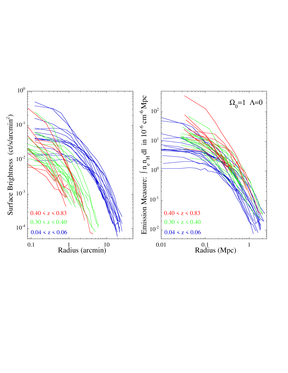
Figure 1: The ROSAT X-ray surface brightness ($S_{\rm X}$) profiles (left panel) and emission measure ($EM$) along the line of sight profiles (right panel) of all (nearby and distant) clusters in the sample. A straight line is drawn between the data points for each cluster for a better visualization of the profiles. The curves are color-coded by redshift. The $S_{\rm X}$ profiles are background subtracted and corrected for vignetting effects. $EM$ is derived from the surface brightness taking into account the $(1+z)^{-4}$ cosmological dimming and the emissivity in the ROSAT band (see Eq. 1). The angular radius is converted to physical radius, assuming $\rm\Omega_{0}=1$ and $\rm h_{50}=1$.

To study cluster evolution, we combined this new distant cluster sample with the sample considered in our previous study of the surface brightness profiles of nearby clusters (Neumann & Arnaud neumann99 (1999),neumann01 (2001)). This nearby cluster sample comprises 15 Abell clusters in the redshift range $0.04<z<0.06$, which were observed in pointing mode with the ROSAT PSPC with a high signal to noise ratio and for which accurate temperature measurements exist from the literature (see Neumann & Arnaud neumann99 (1999) for details).

We emphasize that the study presented here focuses on relatively hot clusters, the minimum temperature for the nearby and distant cluster samples being 3.7 and 3.4 $\rm keV$ respectively.

2.2 Surface brightness profiles

The surface brightness profile of each cluster, $S(\theta)$, was constructed using the standard procedures described in Neumann & Arnaud (neumann99 (1999)). We only considered photons in the energy band 0.5-2.0 keV for the PSPC data and only took into account channels 2-10 for the HRI data, in order to optimize the signal-to-noise (S/N) ratio. We binned the photons into concentric annuli centered on the maximum of the X-ray emission with a width of 15” and 10” per annulus for the PSPC and HRI data respectively. We cut out serendipitous sources in the field of view or cluster substructures, if they show up as a local maximum. The HRI particle background was subtracted from the HRI profiles using the background map constructed for each observation with the method of Snowden et al. (snowden (1998)). The vignetting correction was performed using the exposure maps computed with EXSAS (Zimmermann et al. zimmermann (1994)) for the PSPC data and with the software developed by Snowden (snowden (1998)) for the HRI data. The X-ray background for each pointing was estimated using vignetting corrected data in the outer part of the field of view and subtracted from the profile. A $5\%$($10\%$) systematic error was added quadratically to the statistical error on the PSPC(HRI) background level.

For 5 clusters both HRI and PSPC data were available. We found an excellent agreement between the HRI and PSPC profiles, except for the most inner radial bin, where the effect of the wider PSPC/PSF can be observed. This blurring is clearly negligible at larger radii. If available, we thus always choose the PSPC data, due to its higher intrinsic sensitivity and lower background level, which allow to trace the cluster emission further out.

To avoid too noisy profiles, we rebinned the data, for both the nearby and distant cluster samples, so that the variations of $S(\theta)$ from bin to bin are significantly larger than the corresponding statistical error and thus representative of the cluster shape. Starting form the central annulus, we regrouped the data in adjacent annuli so that i) at least a S/N ratio of $3\sigma$ is reached after background subtraction and ii) the width of the annulus, $\Delta(\theta)$, at radius $\theta$, has a size at least $0.15\leavevmode\nobreak\ \theta$. This logarithmic binning insures a roughly constant S/N ratio for each bin in the outer part of the profiles, where the background can still be neglected (the S/N ratio would be constant for a $\beta$–model with $\beta=2/3$ and no background). The adopted rebinning was found to be a good compromise between the desired accuracy and a reasonable sampling of the profiles.

The resulting surface brightness profiles are shown in Fig. 1 (left panel) for the distant and nearby clusters. For each cluster the data points are connected by a straight line to guide the eye. The profiles are plotted up to the adopted detection limit of $3\sigma$ above background. The corresponding detection radius, as well as the total ROSAT count rate, $CR_{\rm det}$, within this radius is given in Tab. 1 for each cluster. In Fig. 1 and Fig. 2, we color–coded the profiles according to cluster redshift: blue for nearby clusters ($0.04<z<0.06$), green for moderately distant clusters ($0.3<z<0.40$) and red for very distant clusters ($0.40<z<0.83$). Note that this redshift subsampling of the distant cluster sample is for display only and, unless explicitly stated, is not used in the statistical analysis below.

2.3 Emission measure profiles

The emission measure along the line of sight at radius $r$, $EM(r)=\int n_{\rm e}n_{\rm H}\leavevmode\nobreak\ dl$, can be deduced from the X-ray surface brightness, $S(\theta)$:

$$EM(r) = \frac{4\leavevmode\nobreak\ \pi\leavevmode\nobreak\ (1+z)^{4}\leavevmode\nobreak\ S(\theta)}{\epsilon(T,z)}$$ (1)

$$= 4.81\leavevmode\nobreak\ 10^{-7}(1+z)^{4}\left(\frac{S(\theta)}{\rm ct/s/arcmin^{2}}\right)$$

$$\times\left(\frac{\epsilon(T,z)}{\rm ct/s/10^{10}cm^{-5}}\right)^{-1}\leavevmode\nobreak\ {\rm cm^{-6}\leavevmode\nobreak\ Mpc}$$

$$r = d_{\rm A}(z)\leavevmode\nobreak\ \theta$$ (2)

where $d_{\rm A}(z)$ is the angular distance at redshift $z$.

${\epsilon}(T,z)$ is the emissivity in the considered ROSAT band, $[E_{1}-E_{2}]$, taking into account the interstellar absorption and the instrumental spectral response:

$${\epsilon}(T,z)=\int_{E_{1}}^{E_{2}}S(E)e^{-\sigma(E)N_{\rm H}}f_{T}((1+z)E)(1+z)^{2}dE$$ (3)

where $S(E)$ is the detector effective area at energy $E$, $\sigma(E)$ the absorption cross section, $N_{\rm H}$ the hydrogen column density along the line of sight, $f_{T}((1+z)E)$ the emissivity in photons cm³/s/keV at energy $(1+z)E$ for a plasma of temperature $T$. It was computed for each cluster using a redshifted thermal emission model (Mewe et al. mewe1 (1985),mewe2 (1986); Kaastra kaastra (1992); Liedahl et al. liedahl (1995)), the ROSAT response (Zimmermann et al. zimmermann (1994)) and the $N_{\rm H}$ value estimated with the w3nh tools available at HEARSAC (Dickey & Lockman dickey (1990)). The emissivity, ${\epsilon}(T,z)$, depends weakly on cluster temperature and redshift in the ROSAT band (Tab. 1).

The derived $EM(r)$ profiles are shown in the right panel of Fig. 1 for a critical density Universe ($\rm\Omega_{0}=1,\Lambda=0.)$. As will be discussed later, one can already note that the distant clusters appear brighter than the nearby clusters.

3 Theoretical scaling laws

In our derivation of the theoretical emission measure profiles, as a function of redshift and cosmological parameters, we will consider both a flat Universe ($\rm\Omega_{0}+\Lambda=1$) and an open Universe ($\rm\Omega_{0}<1,\Lambda=0$). The matter density parameter at redshift $z$ is noted $\rm\Omega_{\rm z}$; $\rm\Omega_{\rm z}=\rm\Omega_{0}(1+z)^{3}/E^{2}(z)$, where $E^{2}(z)=\rm\Omega_{0}(1+z)^{3}+(1-\rm\Omega_{0}-\Lambda)(1+z)^{2}+\Lambda$.

3.1 The self-similar model

The simplest self-similar model (e.g. Bryan & Norman bryan98 (1998); Eke et al. eke (1998)) assumes that i) at a given redshift the relaxed virialized portion of clusters corresponds to a fixed density contrast as compared to the critical density of the Universe at that redshift ii) the internal structure of clusters of different mass and $z$ are similar.

The virial mass $M_{\rm V}$ and radius $R_{\rm V}$ then scale with redshift and temperature via the well known relations:

$$M_{\rm V} = 2.835\leavevmode\nobreak\ 10^{15}\leavevmode\nobreak\ \beta_{\rm T}^{3/2}\ \Delta_{\rm z}^{-1/2}\ (1+z)^{-3/2}$$ (4)

$$\times\left(\frac{{\rm k}T}{10\ \rm keV}\right)^{3/2}\ \rm h_{50}^{-1}\leavevmode\nobreak\ \leavevmode\nobreak\ \hbox{$M_{\sun}$}$$

$$R_{\rm V} = 3.80\leavevmode\nobreak\ \beta_{\rm T}^{1/2}\ \Delta_{\rm z}^{-1/2}\ (1+z)^{-3/2}$$ (5)

$$\times\left(\frac{{\rm k}T}{10\ \rm keV}\right)^{1/2}\ \rm h_{50}^{-1}\leavevmode\nobreak\ \leavevmode\nobreak\ {\rm Mpc}$$

$${\rm with}$$

$$\Delta_{\rm z} = (\Delta_{\rm c}(\rm\Omega_{\rm z},\Lambda)\rm\Omega_{0})/(18\pi^{2}\rm\Omega_{\rm z})$$ (6)

where $\Delta_{\rm c}(\rm\Omega_{\rm z},\Lambda)$ is the density contrast (a function of $\rm\Omega_{0}$ and $\Lambda$) and $\beta_{\rm T}$ is the normalisation of the virial relation, ${\rm G}M_{\rm V}/2R_{\rm V}=\beta_{\rm T}{\rm k}T$.

The $M_{\rm V}$–$T$ and $R_{\rm V}$–$T$ relations depend on the cosmological parameters through the factor $\Delta_{\rm c}(\rm\Omega_{\rm z},\Lambda)\rm\Omega_{0}/\rm\Omega_{\rm z}$. This factor is constant with redshift and equal to $18\pi^{2}$ for a critical density Universe. Analytical approximations of $\Delta_{\rm c}(\rm\Omega_{\rm z},\Lambda)$, derived from the top-hat spherical collapse model assuming that clusters have just virialized, are given in Bryan & Norman (bryan98 (1998)):

$$\Delta_{\rm c}(\rm\Omega_{\rm z},\Lambda) = 18\pi^{2}+60w-32w^{2}\leavevmode\nobreak\ {\rm for}\leavevmode\nobreak\ \rm\Omega_{0}<1,\Lambda=0$$

$$\Delta_{\rm c}(\rm\Omega_{\rm z},\Lambda) = 18\pi^{2}+82w-39w^{2}\leavevmode\nobreak\ {\rm for}\leavevmode\nobreak\ \rm\Omega_{0}+\Lambda=1$$

$${\rm with}\leavevmode\nobreak\ \leavevmode\nobreak\ w = \rm\Omega_{\rm z}-1$$ (7)

As we consider lower and lower values of the density parameter $\rm\Omega_{0}$, the assumption of recent cluster formation is less and less valid and in principle, the difference between the observing time and the time of collapse has to be taken into account (e.g. Voit & Donahue voit (1998)). If the effective formation epoch of a cluster of a given mass is earlier than the observing time, when the Universe was denser, the actual cluster temperature is underestimated by the recent formation approximation. This effect is expected to increase with decreasing $\rm\Omega_{0}$ and mass of the system. Estimating accurately the impact on the $M_{\rm V}$–$T$ relation (mean relation and scatter) is however not trivial, because it requires a precise modelling of cluster formation history, the growth of clusters by continuous accretion and merger events, and the complex physics of the ICM (Voit voit00 (2000), Afshordi & Cen afshordi (2002)). However, recent analysis of the $M_{\rm V}$–$T$ relation derived from numerical simulations suggest that the effect of formation redshift is negligible, at least when considering measured X–ray temperatures (Mathiesen mathiesen (1998)). We will thus neglect this effect here and use the above equations estimated at the observed cluster redshift.

The constant $\beta_{\rm T}$ depends on the cluster internal structure. Its value can be determined from numerical simulations. The various results agree within typically $\pm 20\%$, with no obvious dependence on cosmological parameters (Henry henry (2000)). As in our previous work (Neumann & Arnaud neumann99 (1999);neumann01 (2001)), we will adopt the normalisation of Evrard et al. (evrard (1996)), $\beta_{\rm T}=1.05$. Note that our results do not depend on the exact value of $\beta_{\rm T}$.

3.2 The theoretical emission measure profiles

The central emission measure along the line of sight is related to the electron density profile of the gas, $n_{\rm e}(r)$, via:

$$EM_{0} = 2\leavevmode\nobreak\ (n_{\rm H}/n_{\rm e})\int_{0}^{R_{\rm V}}n_{\rm e}(r)^{2}\leavevmode\nobreak\ dr$$ (8)

whereas the gas mass is given by:

$$M_{\rm gas} = \mu^{\prime}\leavevmode\nobreak\ {\rm m_{p}}\leavevmode\nobreak\ (n_{\rm H}/n_{\rm e})\leavevmode\nobreak\ 4\pi\leavevmode\nobreak\ \int_{0}^{R_{\rm V}}n_{\rm e}(r)\leavevmode\nobreak\ r^{2}\leavevmode\nobreak\ dr$$ (10)

where ${\rm m_{p}}$ is the proton mass, $\mu^{\prime}=1.347$ and $n_{\rm H}/n_{\rm e}=0.852$, for an ionized plasma with a metallicity of 0.3 solar value. In self-similar models, which we consider here, the density profile can be written:

$$n_{\rm e}(r) = n_{\rm e}(0)\ f_{\rm n}(x)\leavevmode\nobreak\ \leavevmode\nobreak\ \leavevmode\nobreak\ ;x=r/R_{\rm V}$$ (11)

where $x$ is the radius scaled to the virial radius and $f_{\rm n}$ is a universal function, the same for all clusters. By combining the above equations, $EM_{0}$ varies as $EM_{0}\propto Q_{\rm n}M_{\rm gas}^{2}/R_{\rm V}^{5}$, where we have introduced a constant form factor $Q_{\rm n}$, which only depends on the cluster’s ‘universal’ shape:

$$Q_{\rm n} = \frac{\int_{0}^{1}f_{\rm n}^{2}(x)\leavevmode\nobreak\ dx}{9\ \left(\int_{0}^{1}f_{\rm n}(x)\leavevmode\nobreak\ x^{2}\leavevmode\nobreak\ dx\right)^{2}}$$ (12)

Assuming a standard $\beta$–model with $\beta=2/3$ and a scaled core radius of $x_{\rm c}=0.123$, which fits well the scaled profiles of nearby clusters (Neumann & Arnaud neumann99 (1999)), gives $Q_{\rm n}=69.4$.

The scaling law for the central emission measure can now be derived from Eq. 8,10,11 and 12 and the $M_{\rm V}$–$T$ and $R_{\rm V}$–$T$ relations (Eq. 4,5), assuming that all clusters have the same gas mass fraction $f_{\rm gas}$:

$$EM_{0} = 4.1\leavevmode\nobreak\ 10^{-6}\ \left(\frac{\beta_{\rm T}}{1.05}\right)^{1/2}\ \left(\frac{f_{\rm gas}}{0.2}\right)^{2}\ \left(\frac{Q_{\rm n}}{69.4}\right)$$ (13)

$$\times\leavevmode\nobreak\ \Delta_{\rm z}^{3/2}\ (1+z)^{9/2}\ \left(\frac{{\rm k}T}{10\ \rm keV}\right)^{1/2}\rm h_{50}^{3}\ {\rm cm^{-6}Mpc}$$

This assumes that the gas mass scales as the total mass, i.e $M_{\rm gas}\propto T^{1.5}$. The corresponding emission measure profiles can thus be written:

$$EM(r) = EM_{0}\ f_{\rm EM}(r/R_{\rm V})$$ (14)

where $f_{\rm EM}(x)$ is the dimensionless function:

$$f_{\rm EM}(x) = \int_{x}^{1}\frac{f_{\rm n}(u)}{\sqrt{u^{2}-x^{2}}}d(u^{2})$$ (15)

As can be seen from Eq. 5 and Eq. 13, the virial radius decreases with redshift while the central emission measure increases. Clusters of a given mass are denser at high redshift, following the evolution of the Universe mean density. We thus expect that clusters of given temperature appear smaller and brighter with increasing redshift.

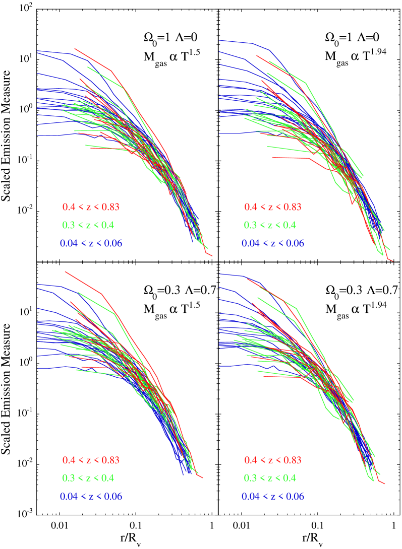
Figure 2: The scaled emission measure along the line of sight as a function of scaled radius for the 40 clusters of the sample in two cosmological models. Top panels: $\rm\Omega_{0}=1.,\Lambda=0$. Bottom panels: $\rm\Omega_{0}=0.3,\Lambda=0.7$. The data points for each cluster are connected by a straight line for a better visualization of the profiles. The curves are color-coded by redshift. The radius is scaled by the virial radius, $R_{\rm V}$, computed using the theoretical scaling law (Eq. 5) with the measured temperature and redshift of the clusters. The emission measure profiles in the left panels have been scaled by $(\Delta_{\rm c}(\rm\Omega_{\rm z},\Lambda)\rm\Omega_{0}/\rm\Omega_{\rm z})^{3/2}(1+z)^{9/2}T^{1/2}$, according to the standard self-similar model (Eq. 18), with $M_{\rm gas}\propto T^{1.5}$. Note the remarkable similarity of the profiles at radii larger than $\sim 0.1R_{\rm V}$. The scaling procedure has significantly decreased the dispersion between the emission measure profiles (compare with the right panel of Fig.1). The right panels correspond to the empirical scaling law assuming $M_{\rm gas}\propto T^{1.94}$, consistent with the slope of the local $L_{\rm X}$–$T$ relation (Neumann & Arnaud neumann01 (2001)). The dispersion is decreased even more as compared to the standard scaling.

3.3 The $L_{\rm X}$–$T$ relation and the empirical scaling law

The bolometric cluster luminosity is given by:

$$L_{\rm X} = \Lambda(T)\int_{0}^{R_{\rm V}}EM(r)2\pi rdr$$ (16)

where the cooling function, $\Lambda(T)$ varies as $\Lambda(T)\propto T^{1/2}$. For the standard self-similar model described above, the bolometric luminosity follows the well known scaling relation:

$$L_{\rm X} \propto \Delta_{\rm z}^{1/2}\ (1+z)^{3/2}\ T^{2}$$ (17)

which is inconsistent with the slope of the observed local $L_{\rm X}$–$T$ relation, $\alpha\sim 2.88$ (e.g Arnaud & Evrard arnaud (1999)).

As already mentioned in the introduction, we found evidence for a steepening of the $M_{\rm gas}$–$T$ relation for hot clusters (Neumann & Arnaud neumann01 (2001)), in our previous study of the nearby cluster sample considered here. A gas mass varying as $M_{\rm gas}\propto T^{1.94}$, instead of $M_{\rm gas}\propto T^{1.5}$, can both explain the observed $L_{\rm X}$–$T$ relation and significantly reduce the scatter in the scaled emission measure profiles, when compared to the standard scaling. In that case, the emission measure scales with temperature as $EM\propto T^{1.38}$, instead of $T^{0.5}$. We will also consider this empirical scaling law in the following section. The dependence of the normalisation on redshift and cosmological parameters remains a priori unchanged and we will assume that the empirical slope of the relation does not evolve with redshift, which is the simplest assumption.

4 Scaled emission measure profiles

4.1 Scaling procedure

As in our previous studies, we scaled the emission measure profiles so that they would lie on top of one another if obeying self-similarity. The scaled emission measure profiles, corresponding to the standard scaling with $z$ and $T$ given Eq. 13, are thus defined as:

$$\widetilde{EM}(x) = \Delta_{\rm z}^{-3/2}(1+z)^{-9/2}\ \left(\frac{{\rm k}T}{10\ \rm keV}\right)^{-1/2}$$

$$\times\leavevmode\nobreak\ \left(\frac{EM(r)}{4.10\leavevmode\nobreak\ 10^{-6}{\rm cm^{-6}Mpc}}\right)$$

$$x = \frac{r}{R_{\rm V}}$$ (18)

where $R_{\rm V}$ is defined by Eq. 5 and the emission measure is derived from the surface brightness via Eq. 1.

To introduce the empirical $EM$–$T$ scaling relation ($EM\propto T^{1.38}$), we simply have to introduce a corrective multiplicative factor of $\propto T^{-0.88}$ to the previous equation:

$$\widetilde{EM}(x) = \Delta_{\rm z}^{-3/2}(1+z)^{-9/2}\ \left(\frac{{\rm k}T}{10\ \rm keV}\right)^{-1.38}$$ (19)

$$\times\leavevmode\nobreak\ \left(\frac{EM(r)}{6.0\leavevmode\nobreak\ 10^{-6}{\rm cm^{-6}Mpc}}\right)$$

For convenience, the corrective factor has been arbitrarily normalized to 1 for a temperature equal to $6.5\ \rm keV$, which is the mean temperature of the sample.

The scaled profiles depend on the assumed cosmological parameters, via the angular distance $d_{\rm A}(z)$ used to convert angular radii to physical radii and via the factor $\Delta_{\rm z}=(\Delta_{\rm c}(\rm\Omega_{\rm z},\Lambda)\rm\Omega_{0})/(18\pi^{2}\rm\Omega_{\rm z})$ appearing in the normalisation of the profiles and of the $R_{\rm V}$–$T$ relation. The variation with redshift of both quantities depends on $\rm\Omega_{0}$ and $\Lambda$. Therefore, if the self-similar evolution model is valid, the scaled profiles of clusters observed at various redshifts will coincide, but only for the correct cosmological parameters.

The scaled profiles can thus be used both to check the validity of the self-similar model and to put constraints on the cosmological parameters, $\rm\Omega_{0}$ and $\Lambda$. This is described in detail in Sect. 5 and further discussed in Sect. 7. To do so, we will use some general properties of the profiles that we outline below.

4.2 Scaled Profiles

The scaled profiles are shown in Fig. 2 for two cosmological models, a critical density Universe $(\rm\Omega_{0}=1)$ and a flat model with $\rm\Omega_{0}=0.3$ and $\Lambda=0.7$. At first sight, distant clusters appear remarkably similar to nearby clusters, once the profiles are scaled. As expected, the difference between the scaled profiles, however, depends on the assumed cosmological parameters. The profiles plotted in the top and bottom panels of Fig. 2 are clearly different, in particular in the relative position of the clusters for the different redshift ranges.

One further notes the large scatter in the scaled profiles in the cluster core ($r<0.1R_{\rm V}$) and the remarkably common shape above typically $0.1-0.2\leavevmode\nobreak\ R_{\rm V}$. This was already noted for nearby clusters (Neumann & Arnaud neumann99 (1999)) and clearly also holds for distant clusters. The large scatter in the core is likely to be due to cooling flows of various sizes. For instance the four clusters with the highest central value, MS 2137.3-2353, RXJ 1347.5-1145, MS 1512 and 3C295, are known, or suspected, to host massive cooling flows. The mass accretion rate, estimated using standard cooling flow models, is as high as $3000{\rm\hbox{$M_{\sun}$}/yrs}$ for RXJ 1347.5-1145 (Schindler et al.  schindler97 (1997) and $500-900{\rm\hbox{$M_{\sun}$}/yrs}$ for 3C295 (Neumann neumann99b (1999)). The presence of a massive cooling flow in MS 1512.4+3647 is indicated by the detection of luminous extended $H_{\alpha}$ emission (Donahue et al.  donahue92 (1992)). No detailed cooling flow analysis is available for MS 2137.3-2353. However, we note that the estimated cooling time for this cluster is about 1/10 of the Hubble time (Allen & Fabian allen98b (1998)) and a clear drop of temperature is observed in the center, similar to the one observed in RXJ 1347.5-1145 (Allen et al.  allen01 (2001)).

A first quantitative check of similarity beyond the core can be made by looking at the dispersion among the profiles at a given radius, for the whole cluster sample. The surface brightnesses are measured at discrete values of the angular radii . To compute the mean value and dispersion of the profiles at any physical or scaled radius, a continuous profile was generated for each cluster using a logarithmic interpolation of the data.

The scaling procedure always significantly reduces the differences among the profiles, as can already be seen by comparing Fig. 1 and Fig. 2. This is a first indication that clusters obey scaling laws up to high redshift. Let us for instance consider the standard scaling with $\rm\Omega_{0}=1$. The relative bi-weight dispersion of the emission measure profiles at a given radius is $\sim 100\%$ between 0.5 and 1 Mpc, whereas the dispersion drops to $\sim 40-45\%$ for the scaled profiles between $0.2$ and $0.5R_{\rm V}$.

Furthermore, in the same range of radii, the scatter is further decreased to $\sim 35-40\%$ for the empirical scaling relation ($EM\propto T^{1.38}$, right panel). This decrease is slightly more pronounced in a low $\rm\Omega_{0}$ Universe. The improvement is not as spectacular as for the local sample alone (a factor of 2 decrease of the scatter). However, this additional $T^{-0.88}$ scaling factor introduces additional noise due to the uncertainties on the temperatures. These errors are particularly large for the distant cluster sample. The fact that there is still an improvement, in spite of this additional noise, suggests that the empirical $EM$–$T$ scaling relation fits better the cluster properties than the standard case, over the redshift range $z=0.04-0.8$. We will thus adopt this empirical scaling relation in the following.

5 Test of self-similarity and constraints on the cosmological parameters

5.1 Method

Our aim is to check, in a quantitative way, the validity of the self-similar model, and set constraints on the cosmological parameters. For that purpose, we need a better statistical estimator than the calculated dispersion of the profiles at a given radius, which we used in the previous section. The relative dispersion is not a global estimator and furthermore does not take into account measurement errors.

We first derived, for each set of cosmological parameters, a scaled reference profile, and an estimate of the intrinsic scatter around it, using the nearby cluster sample data. To do so, we estimated, at any given scaled radius, the mean value of the different scaled $EM$ profiles, together with the corresponding standard deviation, at that specific radius. We computed this reference profile up to the radius for which at least two nearby cluster profiles are still available. Note that measurement errors, which are much less than for the distant cluster sample, can still contribute to the scatter. Analytical fits of the reference scaled profiles (for open and flat Universes) are given in Appendix A.

We then considered the set of data points for the distant cluster sample. Each data point is the scaled emission measure $\widetilde{EM_{i,j}}$ of cluster $j$, measured at the scaled radius $x_{i,j}$, with corresponding $1\leavevmode\nobreak\ \sigma$ errors. The error on the temperature contributes to both the error on $x_{i,j}$ and on $\widetilde{EM_{i,j}}$, while the error on the surface brightness obviously only contributes to the later quantity. These data points are compared to the corresponding reference profile in the left panel of Fig. 4 for a critical density Universe.

If the self-similar model is valid, the distant cluster data points after scaling must be consistent with the reference profile, within the errors. We thus computed the $\chi^{2}$ value of the distant cluster data about the reference curve, for each cosmological model. This $\chi^{2}$ value can be used to assess in the standard way the validity of the underlying self-similar model and to constrain the cosmological parameters, considered as free parameters of the model.

The $\chi^{2}$ computation is not straightforward, because there are non negligible errors on both variables $x$ and $\widetilde{EM}$, these errors are correlated, and the reference curve is not linear. Furthermore, we have to take into account the existence of intrinsic scatter. The computation of $\chi^{2}$ is detailed in Appendix B.

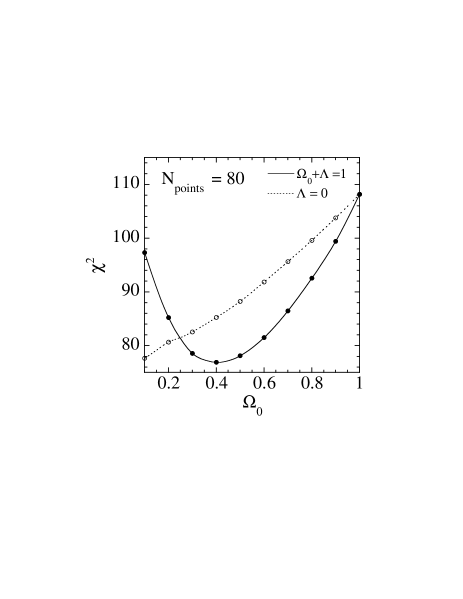
Figure 3: $\chi^{2}$ value of the distant cluster data about the mean scaled emission measure profile of nearby clusters, as a function of $\rm\Omega_{0}$. Full line: flat Universe, $\rm\Omega_{0}+\Lambda=1$. Dotted line: Open Universe, $\Lambda=0$.

Another technical issue is the choice of data points included in the computation of the overall $\chi^{2}$. First, and obviously, only points for which there is a corresponding reference value from the local sample can be included. In practice, very few points are excluded this way, since, for every cosmological model, the distant clusters are usually traced up to smaller scaled radii when compared to nearby clusters. Furthermore, as discussed in the previous section, the core properties are clearly dominated by different physics. It is thus better to exclude the central points to check self-similarity at large radii and to constrain in a more significant way the cosmological parameters. For that purpose, including the central points would be equivalent to add extra noise. We thus considered a fixed number of points, $N_{\rm p}$, defined as the $N_{\rm p}$ most distant from the center in scaled coordinates. Although the relative position of the points depends somewhat on the cosmological parameters, essentially the same data set is compared to the reference curve in all cases. We both considered $N_{\rm p}=80$ and $N_{\rm p}=150$ corresponding respectively to a minimum scaled radius $x=0.2$ and $x=0.1$ for $\rm\Omega_{0}=1$.

Figure 4: Comparison between the scaled emission measure profiles of the distant clusters (data points) and the mean scaled profile determined from the nearby cluster sample ($z=0.04-0.06$, full line) for two cosmological models. The profiles are scaled assuming $M_{\rm gas}\propto T^{1.94}$. The data for the distant clusters are the same as shown in the right panels of Fig. 2 but each data point is now displayed individually with $1\sigma$ error bars on both scaled variables. Open and filled points correspond to clusters in the redshift range $z=0.3-0.4$ and $z=0.40-0.83$, respectively. The dotted lines correspond to the mean profile of nearby clusters, taken as a reference profile, plus or minus the corresponding standard deviation. The bottom panels show the $\chi$ value of individual points about the reference profile, taking into account the correlation between the errors and the dispersion around the reference profile. Left panel: Results for $\rm\Omega_{0}=1,\Lambda=0$. The distant cluster data are not consistent with the nearby cluster data for a critical density Universe. Most of the points lie significantly below the reference profile. Right panel: Results for $\rm\Omega_{0}=0.4$ and $\Lambda=0.6$. Note the good agreement between the scaled emission measure profiles of distant clusters and the mean scaled profile of nearby clusters. There is also no systematic variation of the $\chi$ value with radius, an additional indication of self-similarity in shape.

The variation of the $\chi^{2}$ value with $\rm\Omega_{0}$ is plotted in Fig. 3 for a flat Universe $(\rm\Omega_{0}+\Lambda=1)$ and an open Universe ($\Lambda=0$) for $N_{\rm p}=80$. The individual $\chi$ values for each data point are plotted on the bottom panels of Fig. 4 for a critical Universe (left panel) and for the flat model, $\rm\Omega_{0}=0.4$ and $\Lambda=0.6$, with the lowest $\chi^{2}$ value (right panel).

5.2 Results

For $\rm\Omega_{0}=1$, most of the scaled distant cluster data points fall significantly below the reference curve (Fig. 4, left panel) with an overall $\chi^{2}$ value of 108 for $N_{\rm p}=80$ points. Our data thus allow to exclude the critical density Universe model at the $98\%$ confidence level.

Allowing $\rm\Omega_{0}$ to vary, and considering first a flat Universe, we find an excellent agreement of the distant cluster data with the reference profile for a low density Universe (Fig. 4, right panel). It indicates that hot clusters constitute a homologous family up to high redshifts and strongly supports the underlying self-similar model. The smallest $\chi^{2}$ is reached for $\rm\Omega_{0}=0.4$ ($\Lambda=0.6$), with $\chi^{2}=77$ (reduced $\chi^{2}\sim 1$). Furthermore, no systematic variation of the $\chi$ value with radius is observed, an additional indication of the self-similarity in shape of the profiles (bottom right panel of Fig 4). Interestingly a strong constraint can be set on $\rm\Omega_{0}$: $\rm\Omega_{0}=0.4^{+0.15}_{-0.12}$, with errors given at the $90\%$ confidence level (corresponding to a $\Delta\chi^{2}=2.7$). This result is not sensitive to the number of points considered. For $N_{\rm p}=150$, we obtain similar constraints $\rm\Omega_{0}=0.43^{+0.13}_{-0.11}$, with a slightly better reduced $\chi^{2}$ ($\chi^{2}=115)$. The constraint put on $\rm\Omega_{0}$ for a flat Universe is remarkably consistent with the constrain derived from luminosity distances to SNI: $\rm\Omega_{0}=0.3\pm 0.15$ at the $90\%$ confidence error only taking into account statistical errors (Fig. 7 in Perlmutter et al.  perlmutter (1999)).

We check the robustness of our results on the self-similarity of clusters, with respect to the cluster temperature, by dividing the distant cluster sample in two equal sub–samples. We consider the favored cosmological model ($\rm\Omega_{0}=0.4,\Lambda=0.6$) and only data points with $x>0.08$ (corresponding to $N_{\rm p}=150$ data points in total). We obtain a reduced $\chi^{2}$ of 0.61 ($\chi^{2}=37$ for $61$ data points) for the ${\rm k}T\leq 6.6\leavevmode\nobreak\ \rm keV$ subsample (13 clusters) and a reduced $\chi^{2}$ of 0.88 ($\chi^{2}=78$ for $89$ data points) for the ${\rm k}T>6.6\leavevmode\nobreak\ \rm keV$ subsample (12 clusters). Similarly, splitting the sample with respect to the cluster redshifts, yields a reduced $\chi^{2}$ of 0.82 ($\chi^{2}=80$ for $98$ data points) for the $z\leavevmode\nobreak\ \leq\leavevmode\nobreak\ 0.4$ subsample (15 clusters) and a reduced $\chi^{2}$ of 0.67 ($\chi^{2}=35$ for $52$ data points) for the $z>0.4$ subsample (10 clusters). In conclusion, for the favored cosmology, the distant cluster data for each individual subsample are in excellent agreement with the local reference profile. This reinforces the validity of the considered self-similar model, in particular the redshift dependence of the scaling relations.

An open model ($\Lambda=0$) is also formally consistent with the data. However, the $\chi^{2}$ value keeps decreasing with decreasing $\rm\Omega_{0}$, preventing a strict definition of the constraints. We thus only note that for $\rm\Omega_{0}=0.1$, we obtain a $\chi^{2}=78$, similar to the value for the best model for the flat case. All open models with $\rm\Omega_{0}>0.17$ give $\chi^{2}$ values which are larger than the values corresponding to $90\%$ confidence range of the flat case. Furthermore, we cannot consider arbitrarily low $\rm\Omega_{0}$ values. Obviously $\rm\Omega_{0}$ must be greater than the baryonic density derived from primordial nucleosynthesis ($\Omega_{\rm b}=0.03-0.06$, Suzuki et al. suzuki (2001)). In addition, the various approximations of the scaling models (in particular to compute the over–density) become less and less valid as $\rm\Omega_{0}$ decreases.

5.3 Origin of the constraint on the cosmological parameters

Comparing the scaled emission measure profiles of clusters at different redshifts appears to be a powerful method to constrain the cosmological parameters. To understand better the origin of the constraint, we examine in more details the variation of the scaled profiles, $\widetilde{EM}(x)$, with the cosmological parameters and redshift.

It is useful to first explicitly identify this dependence, which is somewhat complex. The observed quantities are the surface brightness profiles $S(\theta)$, which we correct for the $(1+z)^{4}$ dimming factor. Combining Eq. 18 and Eq. 1, together with Eq. 5 and identifying the relevant factors, we can write:

$$\widetilde{EM}(x) \propto \Delta_{\rm z}^{-3/2}\ \left(1+z\right)^{-9/2}\left[S(\theta)\left(1+z\right)^{4}\right]$$ (20)

$$x \propto \theta\ d_{\rm A}(z)\Delta_{\rm z}^{1/2}\ \left(1+z\right)^{3/2}$$ (21)

Scaling the observed and dimming corrected $S(\theta)$ profile corresponds to translating it in a log-log plane. On the one hand, there is the translation of $\log(d_{\rm A}(z))$ along the x direction related to the conversion of angular radius into physical radius. On the other hand, the cluster cosmological evolution requires an additional translation of $-(3/2)\ \log(\Delta_{\rm z})-(9/2)\ \log(1+z)$ in the y direction, and of $(1/2)\ \log(\Delta_{\rm z})+(3/2)\ \log(1+z)$ in the x direction, i.e along a line of slope -3.

The cosmological parameters appear in the angular distance $d_{\rm A}(z)$ and through the cluster over–density factor $\Delta_{\rm z}$. In the log-log plane, the scaled profiles for two different cosmological models simply differ by translations. At a given redshift, varying the cosmological parameters simply corresponds to the same translation in the log-log plane for all the scaled profiles. The cosmological parameters can thus only be constrained by comparing profiles at different redshifts.

The reference scaled profile is determined from nearby cluster data. This profile depends itself on the cosmological parameters. At low redshifts, increasing $\rm\Omega_{0}$ (for both flat and open models) mainly affects the $\Delta_{\rm z}$ factor, the angular distance being almost insensitive to the cosmological parameters. As $\Delta_{\rm z}$ increases with $\rm\Omega_{0}$, increasing $\rm\Omega_{0}$ moves the scaled profile down and to the right, along the line of slope -3 (defining the scaling translation due to cosmological cluster evolution). This is illustrated in Fig. 5, where we compare the reference profile from the nearby cluster sample for two flat cosmological models ($\rm\Omega_{0}=0.4$, full line, and $\rm\Omega_{0}=1$, dotted line). A remarkable feature is the coincidence of the scaled profiles for the two models at large radii. This is due to the coincidence between the slope of the scaling translation (-3) and the slope of the profile at large radii (thin line in Fig. 5), so that the profile is just translated ‘along it self’. Note that this slope at large radii simply corresponds to a $\beta$–model with $\beta=2/3$, which was shown to fit well the mean profile of nearby clusters (Neumann & Arnaud neumann99 (1999)). At smaller radii, the slope of the profile becomes smaller than -3. As a result, the scaled profile for a high $\rm\Omega_{0}$ value always lies below the corresponding profile for a lower value of $\rm\Omega_{0}$ (Fig. 5).

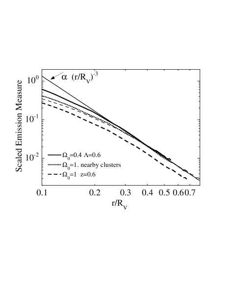
Figure 5: Dependence of the scaled profiles on the cosmological parameters assumed. Thick full line: reference scaled profile from the nearby cluster sample derived for $\rm\Omega_{0}=1$. Dotted line: same for $\rm\Omega_{0}=0.4$, $\Lambda=0.6$. At large radii, the logarithmic slope of the profile is $\sim-3$ (thin full line), corresponding to a $\beta$–model with $\beta=2/3$. Thick dashed line: Scaled profile of a $z=0.6$ cluster one would derived assuming $\rm\Omega_{0}=1$, if the ‘true’ cosmological model was $\rm\Omega_{0}=0.4$, $\Lambda=0.6$, i.e if the ‘true’ scaled profile would follow the dotted line. Thin dashed line: same only taken into account intrinsic cosmological evolution. By using wrong values of the cosmological parameters, the derived profiles of distant and nearby clusters do not coincide any more. The discrepancy is essentially due to the dependence of the derived profiles on the angular distance assumed (see text for full discussion).

Let us now consider a high redshift cluster and assume that the correct cosmological model is a flat Universe with $\rm\Omega_{0}=0.4$. The scaled profile of this cluster, derived for $\rm\Omega_{0}=0.4$, will follow the corresponding reference curve. However, this will not be the case if we assume another $\rm\Omega_{0}$ value. $\Delta_{\rm z}$ varies more rapidly with $\rm\Omega_{0}$ as the redshift increases. As a result, the scaled profile of a high redshift cluster is more affected by a change of $\rm\Omega_{0}$ than the scaled profile of a lower redshift cluster. Taking only into account the translation related to cosmological evolution, we compare the scaled profile of a $z=0.6$ cluster, one would obtain assuming $\rm\Omega_{0}=1$ (thin dashed line in Fig 5) to the corresponding reference curve obtained for this cosmological parameter. The profiles still coincide at large radii, for the reason explained above. At small radii the $z=0.6$ profile is below the reference curve. It must be noted that this effect is small above 0.1 virial radius (less than $20\%$), i.e in the radial range considered. However, at high redshifts, we have also to take into account the variation of the angular distance with $\rm\Omega_{0}$, which decreases with increasing $\rm\Omega_{0}$. The profile has to be further moved to the left, along the x axis, by $\log(d_{\rm A}(z)_{(\rm\Omega_{0}=1)}/d_{\rm A}(z)_{(\rm\Omega_{0}=0.4)})$. At all radii, the profile of the $z=0.6$ cluster (thick dashed line in Fig 5) does not coincide anymore with the reference profile. For a profile shape varying roughly as $x^{-3}$ at large radii, the effect of $d_{\rm A}(z)$ on the scaled emission measure at a given scaled radius is large, $\propto d_{\rm A}(z)^{3}$. At $z=0.6$, the angular distance is about $18\%$ higher for $\rm\Omega_{0}=1$ than for $\rm\Omega_{0}=0.4$ and the profile is $\sim 60\%$ below the corresponding reference profile.

This is exactly what we observe in Fig. 4. For $\rm\Omega_{0}=0.4$ (right panel) distant cluster profiles are consistent with the reference curve. For $\rm\Omega_{0}=1$ (left panel), all the data are moved down. The decrease is more important for distant clusters, which are now systematically lower than the reference curve of nearby clusters, allowing us to exclude this cosmological model. The same reasoning applies for an open Universe. However, the variation of $\Delta_{\rm z}$ and $d_{\rm A}(z)$ with $\rm\Omega_{0}$ is less pronounced for an open Universe than for a flat Universe. The differential effect is less important and the profiles coincide only for lower values of $\rm\Omega_{0}$.

In conclusion, increasing $\rm\Omega_{0}$ moves the scaled profile of a given cluster down and right and decreases the scaled emission measure at a given scaled radius. However, in the radial range considered, the derived scaled profiles of any distant cluster, when compared to the corresponding reference profile, is mostly sensitive to the angular distance $d_{\rm A}(z)$ at the cluster redshift. This is this dependence, which essentially allow to constrain the cosmological parameters, via the well known dependence of $d_{\rm A}(z)$ with $\rm\Omega_{0}$ and $\Lambda$.

6 Evolution of the Lx-T relation

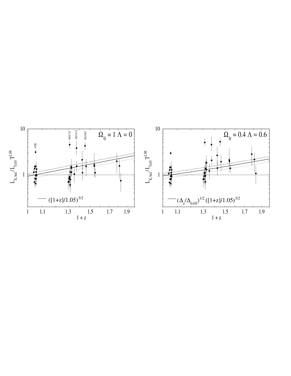
Figure 6: Evolution of the normalisation of the $L_{\rm X}$–$T$ relation for a critical universe (left panel) and a flat Universe with $\rm\Omega_{0}=0.4$ (rtight panel). Data points: Observed bolometric luminosity divided by the luminosity estimated from the local $L_{\rm X}$–$T$ relation and the cluster temperature. Error bars include errors on the luminosity and temperature. Full line: theoretical evolution for the chosen cosmology and the self-similar model of cluster formation. Dotted line: the theoretical curve offset by the intrinsic scatter in $\log(L_{\rm X})$ estimated by Arnaud & Evrard (arnaud (1999)). The evolution of the normalisation of the $L_{\rm X}$–$T$ relation is consistent with the self-similar model for ($\rm\Omega_{0}=0.4$,$\Lambda=0.6$).

We found that the scaled $EM$ profiles of distant clusters coincide with the profile of nearby clusters, using a flat cosmological model with $\rm\Omega_{0}=0.4$. This means that the surface brightness profiles of distant clusters follow the evolution with redshift expected in the self-similar model, for this set of parameters. Since the X–ray luminosity is nothing else than the integral of the surface brightness profile, the evolution of the $L_{\rm X}$–$T$ relation should therefore also comply with this model. We check this point now.

For consistency, we use the bolometric cluster luminosity estimated from the ROSAT data presented here, rather than ASCA. For each cosmological model, the total emission measure within the virial radius is estimated by integrating the profiles up to the detection radius. The contribution beyond that radius was estimated using a $\beta$–model with a slope $\beta=2/3$, normalized to the emission measure at 0.3 virial radius. The luminosity was then estimated using the cooling function computed with a MEKAL model at the cluster temperature (Tab. 1). The ROSAT luminosity values, computed for $\rm\Omega_{0}=1$ are given in Tab. 1. They are in good agreement with the corresponding ASCA estimates from the literature. The median ratio between the two estimates is 0.97, with a standard deviation of $0.2$ and there is no specific trend with redshift.

The considered self-similar model assumes a non-evolving slope of the $EM$–$T$ scaling relation, consistent with the slope (2.88) of the local $L_{\rm X}$–$T$ relation established by Arnaud & Evrard (arnaud (1999)). We thus study the evolution of the normalisation of the $L_{\rm X}$–$T$ relation, assuming a constant slope of 2.88. For each cluster, we define, as in Sadat et al.  (sadat (1998)), the quantity:

$$C_{\rm obs} = \frac{L_{\rm X}}{L_{0.05}\ T^{2.88}}$$ (22)

where $L_{\rm X}$ is the measured bolometric luminosity and $L_{0.05}$ is the normalisation of the local $L_{\rm X}$–$T$ relation, taken from the nearby sample (excluding A780, see below). This normalisation is perfectly consistent with the data of Arnaud & Evrard (arnaud (1999)), the ratio of the two normalizations is 0.99 (for $\rm\Omega_{0}=1$). From Eq. 17, this quantity should evolve as:

$$C_{\rm mod}(z)=\left(\frac{\Delta_{\rm z}}{\Delta_{0.05}}\right)^{1/2}\ \left(\frac{1+z}{1.05}\right)^{3/2}$$ (23)

For consistency, we have normalized the theoretical function, to the value at $z=0.05$, the median redshift of the nearby sample. The observed $C_{\rm obs}$ values, with error bars estimated from the errors on luminosity and temperature, are compared to the theoretical curve, $C_{\rm mod}(z)$, in Fig. 6 for a critical density Universe (left panel) and for our best fit model ($\rm\Omega_{0}=0.4,\Lambda=0.6$, right panel). Four clusters (A780, MS2137, MS1512 and RXJ1347) stand out with particularly high luminosities. Strong cooling flow clusters are known to lie above the $L_{\rm X}$–$T$ relation of weak or non-cooling flow clusters, considered by Arnaud & Evrard (arnaud (1999)). As mentioned above, MS2137, MS1512 and RXJ1347 are indeed known to host strong cooling flows and the same is true for A780. They are thus discarded in the following.

For a critical density Universe most of the data points lie below the theoretical curve, indicating that the distant clusters are under-luminous as compared to the theoretical expectation. This is the same effect as observed for the scaled emission measure, which was also found to be too low as compared to the reference curve. We computed the $\chi^{2}$ value of the distant cluster data points about both the theoretical curve and a constant value of 1, corresponding to no evolution. We assume an intrinsic scatter of 0.13 in $\log(L_{\rm X})$ (Arnaud & Evrard arnaud (1999)). We obtained a reduced $\chi^{2}$ of 2.3 and 1.1, respectively. We thus note that the observed $C_{\rm obs}$ values seem actually consistent with no evolution at all, as found in previous studies of the $L_{\rm X}$–$T$ relation for $\rm\Omega_{0}=1$ (Sadat et al. sadat (1998); Fairley et al. fairley (2000); Reichart et al. reichart (1999)).

On the other hand, the distant cluster data are consistent with the expected evolution of the $L_{\rm X}$–$T$ relation, for $\rm\Omega_{0}=0.4,\Lambda=0.6$. The $\chi^{2}$, in this case, is $\chi^{2}=25$ for 22 clusters (reduced $\chi^{2}_{\rm red}=1.1$). This good $\chi^{2}$ also indicates that the data are consistent with no evolution of the slope of the $L_{\rm X}$–$T$ relation with $z$, as we assume. By comparison, a reduced $\chi^{2}$ of $\chi^{2}_{\rm red}=2.0$ when the data are compared with the no evolution curve. The origin of the improvement, as compared to the $\rm\Omega_{0}=1$ model, is a combination of two factors i) the measured luminosity is higher for lower $\rm\Omega_{0}$, because the estimated distance is larger and ii) the expected evolution of the $L_{\rm X}$–$T$ relation is more modest due the factor $\Delta_{\rm z}$, a decreasing function of $z$. We find that $C_{\rm mod}(z)$, for this cosmological model, is well approximated by a power law over the redshift range considered here ($z=0.-0.83$): $C_{\rm mod}(z)\cong(1+z)^{\eta}$, with $\eta=1.23$. This can be compared with the results of Reichart et al. (reichart (1999)), who assume such a dependence. Their results are based on a compilation of data from the literature for clusters with $z<0.5$. For $\rm\Omega_{0}=0.4,\Lambda=0.6$ ($q_{o}=-0.4$) they found $\eta=1.36^{+0.54}_{-1.22}$, their best fit is thus also in good agreement with the theoretical expectation.

In summary, as expected from our study of the emission measure profiles, the normalisation of the $L_{\rm X}$–$T$ relation, derived for a flat low density Universe, does evolve with redshift. The observed evolution is consistent with the self-similar model of cluster formation.

7 Discussion

7.1 Cluster formation and evolution

We found an excellent agreement, both in shape and normalisation, of the set of scaled profiles of distant clusters with the reference nearby scaled, for a low density flat Universe. This indicates that hot galaxy clusters constitute a homologous family up to high redshift, with the cluster properties scaling with $z$ as expected in the simplest self-similar model. These scaling laws are derived from the assumption that clusters form at fixed density contrast as compared to the critical density of the Universe. Our results thus support this standard picture for the gravitational collapse of the dark matter component.

Consistently, the evolution of the normalisation of the $L_{\rm X}$–$T$ relation was found to comply with the self-similar model for $\rm\Omega_{0}=0.4$, $\Lambda=0.6$. The apparent inconsistency with this model, claimed in some previous studies, was in fact due to the a priori choice of a particular cosmological model ($\rm\Omega_{0}=1$), and is not, per se, an indication of extra-physics. That does not mean that such physics does not exist. We emphasize again that the present study only concerns relatively hot clusters, for which non-gravitational effects like pre-heating is minimal, and that the slopes of the $M_{\rm gas}$–$T$ and $L_{\rm X}$–$T$ relations remain inconsistent with the standard scaling laws. The simplest self-similar model is clearly insufficient to fully describe the properties of the gas component of the ICM. Our data are consistent with no evolution of these slopes with $z$ but much better temperature estimates and larger samples are required for further tests of this point. If this was confirmed, the empirical slopes, together with similarity in shape up to high $z$, have to be explained in terms of the specific gas physics in the picture of structure formation.

7.2 A new method to constrain the cosmological parameters from clusters?

The basic assumption of the method to constrain the cosmological parameters, that we validate a-posteriori, is that clusters form a homologous population. In particular, once scaled according to cluster temperature and redshift, the $EM$ profiles, derived from the observed surface brightness profiles $S(\theta)$, follow a universal function, common to all clusters. This universal function, determined from nearby cluster data, is then used as ‘standard candle’ to constrain the cosmological parameters. The scaled profiles are not used as simple distance indicators, in the strict sense. They do depend on the angular distance, via the conversion of angular radius into physical radius, but, in the self-similar model, the evolution of the scaling relations used in the scaling process also depends on the cosmological parameters. However, we have shown that the second effect is actually negligible. The scaled profiles show a strong dependence on the angular distance, $\propto d_{\rm A}(z)^{3}$ at any given scaled radius. This makes them competitive with other distance indicators like SNI ($\propto d_{\rm A}(z)^{2}$) and indeed, we were able to derive constraints of similar quality.

The method is however by no mean as powerful as the cosmological test based on the evolution of the cluster mass function, $N(M,z)$, which depends much more strongly on $\rm\Omega_{0}$. For instance, the abundance of massive clusters falls by an order of magnitude by $z\sim 0.6$ in a critical density Universe, while it remains unchanged in an $\rm\Omega_{0}=0.3$ Universe (Blanchard & Bartlett blanchard (1998)). However, indirect mass indicators, like $T$ or $L_{\rm X}$, have to be used and the selection function for flux-limited cluster surveys depends on the cluster scaling and structural properties. This $N(M,z)$ test, by nature, thus requires a good knowledge of the cluster scaling properties, and their evolution with $z$, that we study here. The major advantage of the present method is that it is more direct, i.e directly based on observed quantities.

The proposed method suffers, nevertheless, from intrinsic limitations. First, there is some intrinsic dispersion in the cluster properties. The typical dispersion is about $\pm 25\%$, which is not so different from the $\sim 60\%$ in $d_{\rm A}(z)^{3}$ between an $\rm\Omega_{0}=0.4$ ($\Lambda=0.6$) and an $\rm\Omega_{0}=1$ cosmology for a cluster at a redshift as high as $z=0.6$. Therefore, the method requires to consider a large sample of clusters, the scaled profiles of distant clusters will coincide with the reference profile, for the correct values of the cosmological parameters, only in a statistical sense (i.e. on average) and not on a cluster by cluster basis. However, this intrinsic dispersion can be measured and explicitly taken into account. This is done in the present analysis, where the set of distant cluster profiles is compared to the reference profile, with its dispersion, using $\chi^{2}$ statistics.

A more serious concern is that the method is intrinsically model dependent. As for other distance indicators, we cannot exclude that some evolutionary effects, not taken into account, bias the results. In particular, the present analysis relies on the assumption that the slope of both the $EM$–$T$ and $R_{\rm V}$–$T$ relations does not evolve with $z$. If this was not the case, different constrains on $\rm\Omega_{0}$ might be obtained. For instance, a decrease of the $EM$–$T$ relation slope with $z$ would boost the scaled emission measure profiles of high $z$ clusters, as compared to low $z$, and could possibly mimic the effect of a low $\rm\Omega_{0}$ Universe. To further quantify this point, we let the slope of the $EM$–$T$ relation vary with redshift. As a test case, we consider a very simple model. With respect to the standard $EM$–$T$ relation, $EM\propto\Delta_{\rm z}^{3/2}(1+z)^{9/2}T^{1.38}$, the $EM$–$T$ relations at the various redshifts are rotated, around a common reference point of given temperature $T_{\rm p}$, so that the slope varies linearly with $z$: $EM^{\prime}=EM(T/T_{\rm p})^{-(\delta\alpha(z))}$. The slope at $z=0.05$, the median redshift of the nearby cluster sample is kept unchanged and we consider a slope change as high as $\pm 20\%$ at $z=0.8$: $\delta\alpha(z)=\pm 0.37(z-0.05)$, corresponding to $EM\propto T^{1.1}$ or $EM\propto T^{1.66}$ at $z=0.8$. The scaled emission measure profiles are then given by Eq. 19, modified by a multiplicative factor of $(T/T_{\rm p})^{-\delta\alpha(z)}$. The change in the $EM$–$T$ relation, and thus its impact on the $\rm\Omega_{0}$ estimate, depends somewhat critically on $T_{\rm p}$; it is obviously maximal for low values of $T_{\rm p}$. If we take as reference temperature, $T_{\rm p}=3.5\leavevmode\nobreak\ \rm keV$, the minimum temperature of the sample, the scaled emission measure of a $10\leavevmode\nobreak\ \rm keV$ cluster at $z=0.8$ is increased by about $35\%$, for a $20\%$ decrease in slope. As expected, higher $\rm\Omega_{0}$ values are then derived: $\rm\Omega_{0}=0.6^{+0.17}_{-0.15}$ (flat Universe). If instead we assume a steepening of the $EM$–$T$ relation with $z$, we obtain $\rm\Omega_{0}=0.25\pm 0.11$. Both evolution models are consistent with the data, the corresponding reduced $\chi^{2}$ is not significantly different from the one obtained for the standard model. We note however that, in both cases, a critical density Universe remains excluded. Furthermore, when we take $T_{\rm p}=6.5\leavevmode\nobreak\ \rm keV$, the median temperature of the sample, the slope evolution has a negligible effect on the derived parameters: we obtain $\rm\Omega_{0}=0.47\pm 0.14$ and $\rm\Omega_{0}=0.34^{+0.15}_{-0.11}$ for a $+/-20\%$ change in slope, respectively. This systematic effect is twice smaller than the statistical errors on the $\rm\Omega_{0}$ value. Finally, we also checked the effect of a similar change in the slope of the $R_{\rm V}$–$T$ relation. The effect is similarly negligible: we obtain $\rm\Omega_{0}=0.30^{+0.15}_{-0.09}$ and $\rm\Omega_{0}=0.47^{+0.15}_{-0.13}$ for a $20\%$ increase and decrease of the slope respectively.

Our conclusions also depend on the assumed $EM$–$T$ relation, because we are not considering clusters of similar temperatures at all redshifts. The median temperature is $5.8\leavevmode\nobreak\ \rm keV$ for the nearby sample, and $6.6\leavevmode\nobreak\ \rm keV$ and $7.9\leavevmode\nobreak\ \rm keV$ for distant clusters in the redshift ranges $0.3$–$0.43$ and $0.45$–$0.83$, respectively. For a shallower $EM$–$T$ relation, like the standard scaling relation, most of the scaled profiles of distant clusters, lie above the scaled profiles of nearby cluster for $\rm\Omega_{0}=0.3$ (Fig. 2). In that case, a better agreement between the distant cluster data and the nearby cluster data is obtained for $\rm\Omega_{0}=1$ than for $\rm\Omega_{0}=0.3$. However, we emphasize again that the standard scaling law is not consistent with the slope of the $L_{\rm X}$–$T$ relation and that the adopted scaling relation decreases significantly the scatter of the scaled profiles.

Nevertheless, a precise determination of the scaling with temperature, and of its possible evolution, remains essential to achieve a fully consistent description of cluster evolution and to assess possible systematic errors on the cosmological parameters. Again, the quality of the present data is rather insufficient for high precision tests. Finally, there will always remain the possibility of a degeneracy between the evolution of the cluster properties and the variation of the angular distance with redshift. Such systematic errors can only be assessed by comparing the results obtained by various methods. The good agreement obtained between our results and the constraints based on the luminosity distance of SNI is an encouraging sign that both methods are unbiased and the underlying models correct.

7.3 Comparison with previous work based on the size-temperature relation

The cosmological parameters can also be constrained, as proposed by Mohr et al. (mohr00 (2000)), using the isophotal size - temperature (ST) relation. Mohr et al. (mohr00 (2000)) showed that the normalisation of this relation is insensitive to cluster cosmological evolution, considering the same model than in the present study. Their test of the cosmological parameters is thus made via the dependence of the size on the angular distance. Both this method and ours thus use quantities derived from cluster surface brightness profiles, as distance indicators.

The main difference between the two methods is that we consider scaled quantities rather than physical quantities. At large radii, considered by Mohr et al. (mohr00 (2000)), this is equivalent. Due to the coincidence between the slope of the scaling translation related to cluster cosmological evolution and the slope of the profiles (see Sect. 5.3), the profiles of all clusters coincide at large radii, both in the scaled space and in the physical space. This is the origin of the invariance of the isophotal size with redshift (the arguments developed by Mohr et al.  (mohr00 (2000)) are actually similar). For an isophotal size evaluated from cluster images, the method of Mohr et al.  (mohr00 (2000)) is equivalent, in our approach, to consider only data points at a given scaled emission measure.

Our method, where we consider the whole set of data points, can thus be regarded as a generalization of the method proposed by these authors. Note that, by working with scaled quantities, we are able to consider data at small radii, where cosmological evolution has to be taken into account (even if it does not depend sensitively on the cosmological parameters). The method we propose presents several advantages. Obviously tighter constrains can be obtained by considering the whole set of data points. No parametric fit of the surface brightness profiles, as the one introduced by Mohr et al. (mohr00 (2000)), is required. Furthermore, it allows a more complete test of the underlying self-similar model.

We stress on the agreement between the results obtained Mohr et al. (mohr00 (2000)) and ours. Both studies exclude a critical density Universe. Low $\rm\Omega_{0}$ values are favored, somewhat lower when we use the evolution of the ST relation. One also notes that lower $\rm\Omega_{0}$ values are favored for an open model than for a flat model.

8 Conclusion

In this work based on ROSAT data and published ASCA temperatures we study the surface brightness profiles of a sample of hot (${\rm k}T>3.5\leavevmode\nobreak\ \rm keV$) galaxy clusters, covering a redshift range $z=0.04-0.83$. For both open and flat cosmological models, the derived emission measure profiles are scaled according to the self-similar model of cluster formation. We use the standard scaling relations of cluster properties with redshift. The physical radius is normalized to the virial radius, estimated from the classical virial relation. The slope of the $EM$–$T$ relation depends on the assumed slope of the $M_{\rm gas}$–$T$ relation. We consider both the standard scaling relation $M_{\rm gas}\propto T^{1.5}$ and the empirical local relation $M_{\rm gas}\propto T^{1.94}$ (Neumann & Arnaud (neumann01 (2001)), assuming the slope does not evolve with $z$.

Our analysis of the scatter of the scaled profiles, suggests that the empirical slope of the $M_{\rm gas}$–$T$ relation fits better the cluster properties than the standard value, over the whole redshift range $z=0.04-0.8$. As for nearby clusters, a large dispersion in the central core is observed, and we therefore consider only the region above typically $0.1R_{\rm V}$.

Applying the empirical $EM$–$T$ relation, the set of scaled profiles of the distant cluster sample are compared to the average scaled profile of nearby clusters, using a $\chi^{2}$ test. An excellent agreement, both in shape and normalisation, of the distant cluster data with this reference nearby scaled profile is obtained for a flat low density Universe (see also below). Consistently, the evolution of the normalisation of the $L_{\rm X}$–$T$ relation was found to comply with the self-similar model. The apparent inconsistency with this model, claimed in some previous studies, was in fact due to the a priori choice of a particular cosmological model ($\rm\Omega_{0}=1$).

This indicates that hot galaxy clusters constitute a homologous family up to high redshifts and supports the standard picture for the gravitational collapse of the dark matter component. However, the simplest self-similar model is insufficient to fully describe the properties of the gas component of the ICM, as indicated by the non-standard slope of the $M_{\rm gas}$–$T$ (and $L_{\rm X}$–$T$ ) relation. If confirmed, this slope, together with similarity in shape up to high $z$, have to be explained in terms of the specific gas physics in structure formation scenario.

Because of the intrinsic regularity of the hot cluster population, we showed that the scaled emission measure profile, determined from nearby cluster data, can be used as ‘standard candle’ to constrain the cosmological parameters, the correct cosmology being the one for which the profiles at different redshifts coincide. The scaled profiles of distant clusters, as compared to the reference profile, mostly depend on the angular distance, as $d_{\rm A}(z)^{3}$, making them powerful distance indicators. The method is, in addition, more powerful than the test based on the size–temperature relation (Mohr et al.  mohr00 (2000)), because it utilizes the full information contained in the cluster profiles, rather than a particular point of the profiles.

Using this new method, we were able to exclude a critical-density model ($\Omega_{0}=1$) (at 98% confidence level). The data favor a flat Universe with a low matter density, even if the open model is not formally excluded. We find a value of $\Omega_{0}=0.40^{+0.15}_{-0.12}$ (at 90% confidence level). This test relies on the fact that we are using the right scaling relations, in particular for the $EM$–$T$ relation. It is thus, by nature, a model dependent method, although the model can be to some extent, validated a posteriori.

At this stage, our proposed method has to be taken more in terms of an independent consistency check of the constraints on cosmological parameters rather than “an ultimate cosmological test”. The constraint derived on $\rm\Omega_{0}$ is in remarkable agreement with the constraint obtained from luminosity distances to SNI (Perlmutter et al. perlmutter (1999)) or from combined analysis of the power spectrum of the 2dF galaxy redshift Survey and the CMB anisotropy (Efstathiou et al.  efstathiou (2002); see also Melchiorri et al.  melchiorri (2000); Stompor et al.  stompor (2000); de Bernardis et al.  debernardis (2002); Pryke et al.  pryke (2001) and references therein). This is an additional sign that we are entering an era where cosmological tests converge and we can expect that soon the cosmological parameters will be accurately known. In this context, cluster scaling and structural properties will be more adapted to test the physical processes in the structure formation picture. Significant progresses in this field require high quality data with measurements down to the virial radius that will be provided by the new generation of X-ray observatories (Chandra and XMM-Newton). They also require a large sample of distant and nearby clusters so that i) the intrinsic dispersion is pinned down, ii) we improve our knowledge of the local relations and the temperature and dark matter profiles, and iii) we fully assess the evolution with $z$.

Appendix A Analytical fit of the reference scaled profiles

For a critical Universe the reference profile derived from the set of nearby cluster profiles is well fitted by a $\beta$–model above a scaled radius of $x=0.1$:

$$\widetilde{EM}(x) = \widetilde{EM}_{0}\left[1+\left(\frac{x}{x_{\rm c}}\right)^{2}\right]^{-3\beta+0.5}$$ (24)

with $\widetilde{EM}_{0}=0.945$, $x_{\rm c}=0.116$ and $\beta=0.67$. This analytical formula is accurate to $\sim 7\%$ (with typical errors less than $5\%$) in the range $x=0.1$–$0.7$. We emphasize that this formula must not be used for lower values of x (where the scatter increases and the profiles are on average more peaked), as well as above $x=0.7$, corresponding to the last measured point.

The individual cluster scaled profiles, derived from the observed surface brightness profiles, depend on the cosmological parameters, via the factor $\Delta_{\rm z}$ and the angular distance, as given in Eq. 21. The reference profile, for any cosmological model, is well approximated by simply scaling the $\rm\Omega_{0}=1$ reference profile, with the $\Delta_{\rm z}$ and $d_{\rm A}(z)$ factors estimated at $z=0.05$, the mean redshift of the sample. The reference profile is thus given by a $\beta$–model (Eq. 24) with:

$$\widetilde{EM}_{0} = 0.945\leavevmode\nobreak\ \Delta_{0.05}^{-3/2}$$ (25)

$$x_{\rm c} = 0.116\leavevmode\nobreak\ \Delta_{0.05}^{1/2}\leavevmode\nobreak\ f_{\rm{d_{A}}}$$ (26)

$$\beta = 0.67$$ (27)

where $f_{\rm{d_{A}}}$ is the angular distance normalised to its value for $\rm\Omega_{0}=1$. The $\Delta_{0.05}$ factor is given Eq. 6 and Eq. 7, with $z=0.05$. It is accurately (within less than $0.2\%$) aproximated by the following polynomial expression:

$$\Delta_{0.05} = 1-0.365(\rm\Omega_{0}-1)-0.174(\rm\Omega_{0}-1)^{2}\leavevmode\nobreak\ {\rm for}\leavevmode\nobreak\ \rm\Omega_{0}<1,\Lambda=0$$

$$\Delta_{0.05} = 1-0.522(\rm\Omega_{0}-1)-0.199(\rm\Omega_{0}-1)^{2}\leavevmode\nobreak\ {\rm for}\leavevmode\nobreak\ \rm\Omega_{0}+\Lambda=1$$

Similarly the $f_{\rm{d_{A}}}$ factor can be aproximated by:

$$f_{\rm{d_{A}}} = 1+1.25\leavevmode\nobreak\ 10^{-2}(\rm\Omega_{0}-1)\leavevmode\nobreak\ {\rm for}\leavevmode\nobreak\ \rm\Omega_{0}<1,\Lambda=0$$

$$f_{\rm{d_{A}}} = 1+3.75\leavevmode\nobreak\ 10^{-2}(\rm\Omega_{0}-1)\leavevmode\nobreak\ {\rm for}\leavevmode\nobreak\ \rm\Omega_{0}+\Lambda=1$$ (29)

The overall accuracy is similar to the accuracy obtained for the critical Universe reference profile, for $\rm\Omega_{0}>0.1$. Again we emphasize that the analytical formula must only be used between $x_{\rm min}=0.1\Delta_{0.05}^{1/2}f_{\rm{d_{A}}}$ and $x_{\rm max}=0.7\Delta_{0.05}^{1/2}f_{\rm{d_{A}}}$.

Appendix B Computation of the $\chi^{2}$ value

Here, we describe the way we compute the $\chi^{2}$ value used to compare the set of scaled emission measure profiles of distant clusters to the reference profile.

The data consist of a set of scaled emission measure, $y_{k}=\widetilde{EM_{k}}$, measured at the scaled radius $x_{k}$. These quantities are derived from the surface brightness, $SB_{k}$, at angular radius $\theta_{k}$ (corresponding to the scaled radius $x_{k}$) and the temperature of the specific cluster, $T_{k}$:

$$y_{k} \propto SB_{k}\leavevmode\nobreak\ T_{k}^{\alpha}$$ (30)

$$x_{k} \propto T_{k}^{1/2}$$ (31)

where $\alpha$ is the slope of the $EM$–$T$ relation. The corresponding errors, $\sigma_{y_{k}}$ and $\sigma_{x_{k}}$ are:

$$\frac{\sigma_{x_{k}}}{x_{k}} = \frac{1}{2}\ \frac{\sigma_{T_{k}}}{T_{k}}$$ (32)

$$\frac{\sigma_{y_{k}}^{2}}{y_{k}^{2}} = \frac{\sigma_{SB_{k}}^{2}}{SB_{k}^{2}}+\alpha^{2}\frac{\sigma_{T_{k}}^{2}}{T_{k}^{2}}$$ (33)

where $\sigma_{T_{k}}$ and $\sigma_{SB_{k}}$ are the uncertainties on $T_{k}$ and $SB_{k}$ respectively. The errors on $x_{k}$ and $y_{k}$ are thus correlated through the error on the temperature. The correlation factor $\rho_{k}$ is:

$$\frac{\rho_{k}\sigma_{x_{k}}\sigma_{y_{k}}}{x_{k}y_{k}} = \frac{\alpha}{2}\ \frac{\sigma_{T_{k}^{2}}}{T_{k}^{2}}$$ (34)

Let us note $Y=f(X)$ the equation of the reference curve to which this data set is compared. In practice, it is given in tabular form and the data for any value of $X$ is obtained by interpolation. The $\chi^{2}$ expression can be found in York (york (1969)) for the case of correlated errors:

$$\chi^{2} = \sum_{k=1}^{N}S_{k}$$ (35)

where $N$ is the number of data points and $S_{k}$ the distance of the data point $k$ to the reference curve, which is obtained by minimizing over $X$ the function:

$$S_{k}(X) = \frac{1}{1-\rho_{k}^{2}}\left[\frac{\left(x_{k}-X\right)^{2}}{\sigma_{x_{k}}^{2}}\leavevmode\nobreak\ +\frac{\left(y_{k}-f(X)\right)^{2}}{\sigma_{y_{k}}^{2}}\right.$$ (36)

$$\leavevmode\nobreak\ \leavevmode\nobreak\ \leavevmode\nobreak\ \leavevmode\nobreak\ \leavevmode\nobreak\ \leavevmode\nobreak\ \leavevmode\nobreak\ \leavevmode\nobreak\ \leavevmode\nobreak\ \leavevmode\nobreak\ \leavevmode\nobreak\ \left.-2\rho_{k}\frac{\left(x_{k}-X\right)\left(y_{k}-f(X)\right)}{\sigma_{x_{k}}\sigma_{y_{k}}}\right]$$

Since the reference function is not linear, this minimization, which actually determines the ‘closest’ reference point, is done numerically. Up to this stage, we have not taken into account the dispersion, $\sigma_{f(X)}$ at radius $X$, observed around the reference curve. This is done by adding quadratically this dispersion to $\sigma_{y_{k}}$. Eq. 34 and Eq. 36 remain the same, where $\sigma_{y_{k}}$ is replaced by $\sqrt{\sigma_{y_{k}}^{2}+\sigma_{f(X)}^{2}}$.

References

- (1) Afshordi N., Cen R., 2002, ApJ, 564, 669
- (2) Allen, S.W., Fabian, A.C., 1998, MNRAS, 297, L57
- (3) Allen, S.W., Fabian, A.C., 1998, MNRAS, 297, L63
- (4) Allen, S.W., Schmidt R.W., Fabian, A.C., 2001, MNRAS, 328, L37
- (5) Arnaud, M., Evrard, A.E. 1999, MNRAS, 305, 631
- (6) Arnaud, M., 2001, in the Proceedings of the XXIth Moriond Astrophysics Meeting ”Clusters of galaxies and the high redshift Universe Observed in X-rays” (March 2001), to appear
- (7) Bialek, J.J., Evrard, A.E., Mohr, J.J. 2001, ApJ, 555, 597
- (8) Blanchard, A., Bartlett, J., 1998, A&A., 332, L49
- (9) Borgani, S., Governato, F., Wadslay, J. et al. , 2001, ApJ, 559, L71
- (10) Brighenti, F., Mathews, W.G., 2001, ApJ, 553, 103
- (11) Bryan, G.L., Norman, M.L. 1998, ApJ, 495, 80
- (12) Bryan,G.L., 2000, ApJ, 544,L1
- (13) de Bernardis, P., Ade, P., Bock, J. et al. 2002, ApJ, 564, 559
- (14) Della Ceca, R., Scaramella, R., Gioia, I.M., Rosati, P., Fiore, F, Squires, G., 2000, A&A, 353, 498
- (15) Dickey, J.M., Lockman, F.J., 1990, ARA&A, 28, 215
- (16) Donahue, M., Stocke, J. T., Gioia, I. M., 1992, ApJ, 385, 49
- (17) Donahue, M., Mark Voit G., Scharf C.A., Gioia I., Mullis C.R., Hughes J.P., Strocke J., 1999, ApJ, 527, 525
- (18) Efstathiou, G., Moody, S., Peacock, J., et al, 2002, MNRAS, 330, L29
- (19) Eke, V.R., Navarro, J.F., Frenk, C.S. 1998, ApJ, 503, 569
- (20) Ettori S., Fabian A., 1999, MNRAS, 305, 834
- (21) Evrard A.E., Henry J.P, 1991, ApJ, 383, 95
- (22) Evrard, A. E., Metzler, C. A., Navarro, J. F., ApJ, 469, 494
- (23) Fairley, B.W., Jones, L.R., Scharf, C., Ebeling H., Perlman, E., Horner, D., Wegner, G., Malkan, M., 2000, MNRAS, 315, 669
- (24) Finoguenov, A., Reiprich, T. H., Böhringer, H., 2001, A&A, 368, 749
- (25) Gioia, I., Henry, J.P., Mullis, C.R., Ebeling, H., Wolter, A., 1999, ApJ, 117, 2608
- (26) Hattori, M., Ikebe, Y., Asaoka, I., et al. , 1997, Nature, 388, 146
- (27) henry, J.P., 2000, ApJ, 534, 565
- (28) Horner, D.J., Mushotzky R.F., Scharf C.A., ApJ, 520, 78
- (29) Hughes, J.P., Birkinshaw, M., 1998, ApJ, 501,1
- (30) Irwin J.A., Bregman J.N., 2000, ApJ, 538, 543
- (31) Jeltema, T.E, Canizares, C.R., Bautz, M.B. et al. , 2001, ApJ, 562, 124
- (32) Kaastra J.S., 1992, An X-ray spectral Code for Optically Thin Plasmas, Internal SRON-Leiden Report, updated version 2.0
- (33) Kaiser, N. 1986, MNRAS, 222, 323
- (34) Kaiser, N. 1991, ApJ, 383, 104
- (35) Liedahl, D.A., Osterheld, A.L., and Goldstein, W.H. 1995, ApJL, 438, 115
- (36) Lloyd-Davies, E.J., Ponman, T.J., Cannon, D.B. 2000, MNRAS, 315, 689
- (37) Lowenstein, M., 2000, ApJ, 532, 17
- (38) Markevitch, M., Forman, W.R., Sarazin, C.L., Vikhlinin, A. 1998, ApJ 503, 77
- (39) Markevitch, M. 1998, ApJ 504, 27
- (40) Mathiesen, B.J., 2001, MNRAS, 326, L1
- (41) Matsumoto, H., Tsuru, T.G., Fukazawa, Y. et al. , 2000, PASJ, 52, 153
- (42) Melchiori, A., Ade, P., de Bernardis P. et al. , 2000, ApJ, 536, L63
- (43) Mewe, R., Gronenschild, E.H.B.M., and van den Oord, G.H.J. 1985, A&AS, 62, 197
- (44) Mewe, R., Lemen, J.R., and van den Oord, G.H.J. 1986, A&AS, 65, 511
- (45) Mohr, J.J., Evrard, A.E. 1997, ApJ, 491, 38
- (46) Mohr, J.J., Mathiesen, B., Evrard, A.E., 1999, ApJ, 517, 627
- (47) Mohr, J.J., Reese, J.J., Ellingson E. et al. 2000, ApJ, 544, 109
- (48) Muanwong, O.,Thomas, P.A., Kay, S.T. et al. , 2001, ApJ, 552, L27
- (49) Mushotzky, R.F., Scharf, C.A., 1997, ApJ, 482, L13
- (50) Navarro, J.F., Frenk, C.S., White, S.D.M., 1997, ApJ, 490, 493
- (51) Neumann, D.M., Arnaud, M. 1999, A&A, 348, 711
- (52) Neumann, D.M. 1999, ApJ, 520, 87
- (53) Neumann, D.M., Arnaud, M. 2000, ApJ, 542, 35
- (54) Neumann, D.M., Arnaud, M. 2001, A&A, 373, L33
- (55) Nevalainen, J., Markevitch, M., Forman, W., 2000, ApJ, 532, 694
- (56) Ota , 1998, ApJ, 495, 170
- (57) Pearce F.R., Thomas P.A., Couchman H.M.P, Edge A.C., 200, MNRAS, 317, 1029
- (58) Pen, U., 1997, New Astronomy, 2, 309
- (59) Perlmutter, S., Aldering, G., Goldhaber, G et al. , 1999, ApJ, 517, 565
- (60) Ponman, T.J., Cannon, D.B., Navarro, J.F. 1999, Nature 397, 135
- (61) Pierre, M., Matsumoto, H., Tsuru, T., Ebeling, H., Hunstead, R., 1999, A&ASupl., 136, 173
- (62) Pryke, C., Halverson, N.W., Leitch, E.M. et al. , 2001, submitted to ApJ, astro-ph/0104490
- (63) Reichart, D.E., Castander, F.J., Nichol, R.C., 1999, ApJ, 516, 1
- (64) Rines, K., Forman, W., Pen U., et al. , 1999, ApJ, 517, 70
- (65) Sadat, R., Blanchard, A., Oukbir J., 1998, A&A, 329, 21
- (66) Schindler, S., Hattori, M., Neumann, D. M., Böhringer, H. 1997, A&A, 317, 646
- (67) Schindler, S., M., Wambsganss, 1997, A&A, 322, 66
- (68) Schindler, S., Belloni, P., Ikebe, Y., Hattori, M., Wambsganss, J., Tanaka, Y., 1998, A&A, 338, 843
- (69) Schindler, S., 1999, A&A, 349, 435
- (70) Snowden, S.L., 1998, ApJS, 117, 233
- (71) Stompor, R., Abroe, M., Ade , P. et al. , 2001, ApJ, 561, L7
- (72) Suzuki, T.K., Yoshii, Y., Beers, T.C., 2000, ApJ, 540, 99
- (73) Teyssier, R., Chièze, J.P., Alimi, J.M. 1997, ApJ, 480, 36
- (74) Tozzi P., Norman C., 2001, ApJ 546, 63
- (75) Valageas, ,P., Silk, J. 1999, A&A 347,1
- (76) Vikhlinin, McNamara, B.R., Forman, W. et al. , 1998, ApJ, 498, L21
- (77) Vikhlinin, A., Forman, W., Jones, C., 1999, ApJ, 525, 47
- (78) Voit, G.M, Donahue, M., 1998, ApJ, 500, L111
- (79) Voit, G.M, 2000, ApJ, 543, 113
- (80) Wu K.K.S, Fabian, A.C., Nulsen, P.E.J., 2000, MNRAS, 318, 889
- (81) Xu H., Jin G., Wu X.P., 2001, ApJ, 553, 78
- (82) York, D., 1969, Earth and Planetary Science Letters, 5, 320
- (83) Zimmermann, H.U., Becker W., Belloni, T., Döbereiner, S., Izzo, C., Kahabka, P., Schwentker, O., 1994, ”EXSAS User’s Guide”, MPE report 257, October 1994