THE FATE OF THE FIRST GALAXIES. II.
EFFECTS OF RADIATIVE FEEDBACK

Abstract

We use 3D cosmological simulations with radiative transfer to study the formation and evolution of the first galaxies in a $\Lambda CDM$ cosmology. The simulations include continuum radiative transfer using the “Optically Thin Variable Eddington Tensor” (OTVET) approximation and line-radiative transfer in the H₂ Lyman-Werner bands of the UV background radiation. Chemical and thermal processes are treated in detail, particularly the ones relevant for H₂ formation and destruction.

We find that the first luminous objects (“small-halos”) are characterized by bursting star formation (SF) that is self-regulated by a feedback process acting on cosmological instead of galactic scales. The global star formation history is regulated by the mean number of ionizing photons that escape from each source, $\epsilon_{UV}$$\langle f_{esc}\rangle$. It is almost independent of the assumed star formation efficiency parameter, $\epsilon_{*}$, and the intensity of the dissociating background. The main feedback process that regulates the SF is the re-formation of H₂ in front of H ii regions and inside relic H ii regions. The H ii regions remain confined inside filaments, maximizing the production of H₂ in overdense regions through cyclic destruction/reformation of H₂. If $\epsilon_{UV}$$\langle f_{esc}\rangle$ $>10^{-7}/\epsilon_{*}$ the SF is self-regulated, photo-evaporation of “small-halo” objects dominate the metal pollution of the low density IGM, and the mass of produced metals depends only on $\langle f_{esc}\rangle$. If $\epsilon_{UV}$$\langle f_{esc}\rangle$ $\lower 2.15277pt\hbox{$\;\buildrel<\over{\sim}\;$}10^{-7}/\epsilon_{*}$, positive feedback dominates, and “small-halo” objects constitute the bulk of the mass in stars and metals at least until redshift $z\sim 10$. “Small-halo” objects cannot reionize the universe because the feedback mechanism confines the H ii regions inside the large scale structure filaments. In contrast to massive objects (“large halos”), which can reionize voids, “small-halo” objects partially ionize only the dense filaments while leaving the voids mostly neutral.

1 Introduction

In cold dark matter (CDM) cosmologies, “small-halo” galaxies are believed to be the first luminous objects formed in the universe. Defined as small mass protogalaxies, “small-halo” objects have virial temperature $T_{vir}<10^{4}$ K and rely on H₂ line cooling to form stars. The first generation of stars is necessarily metal-free, as all elements heavier than Li are produced in the cores of stars or by supernova (SN) explosions. In the literature Population III is often used to refer to both metal-free stars and to protogalaxies with $T_{vir}<10^{4}$ K. In order to avoid this confusion, we use the term “small-halo” objects instead of the widely used “Population III objects” throughout our paper. For instance, the stars in a “small-halo” object are not necessarily Population III because the interstellar medium (ISM) could be polluted by metals rather quickly. In this paper, we use synthetic stellar energy distributions (SEDs) calculated for metal-free stars, which for brevity we call Population III SEDs, and SEDs typical of low-metallicity stars, which we call Population II SEDs. Although the SED does not change the star formation (hereafter SF) history, we find that the H₂ abundance in the intergalactic medium (IGM) depends on it.

In this paper, the second in a series on the formation and evolution of the first galaxies, we focus on the mechanisms responsible for the the self-regulation of star formation in “small-halo” objects. In Ricotti, Gnedin, & Shull (2002) (Paper I) we discussed the numerical methods and the physics included in the simulations used in this paper. From resolution studies we found that our largest simulations seem to be close to numerical convergence. These models are the first 3D cosmological simulations to include the physics necessary to study the formation of “small-halo” objects and their radiative feedback self-consistently. Mechanical feedback from SN explosions and stellar winds is not included, as it is the subject of a separate paper. The main new ingredients are the inclusion of continuum radiative transfer and line radiative transfer in the Lyman-Werner bands. A number of potentially relevant physical processes are included as well: secondary ionizations of H and He, detailed H₂ chemistry and cooling processes, heating by Ly$\alpha$ resonant scattering, H and He recombination lines, metal production, and radiative cooling. The SED of the sources is consistent with the choice of the escape fraction of ionizing radiation, $\langle f_{esc}\rangle$. The results of our simulations are considerably different from previous models of the formation of “small-halo” objects. These previous works were semi-analytic treatments (Haiman, Rees, & Loeb, 1997, 2000; Ciardi et al., 2000) or 3D simulations (Machacek, Bryan, & Abel, 2001) without radiative transfer. In contrast to previous studies, we find that the formation of “small-halo” objects is not suppressed by the H₂ dissociating background. The reason for this difference is that these earlier studies did not include a primary mechanism of positive feedback for the formation of “small-halo” objects.

Prior to our work, it was widely thought that the main feedback mechanism that regulates “small-halo” formation is the build-up of the H₂ dissociating background. Indeed, the dissociating background can suppress or delay the formation of “small-halo” objects if H₂ is not reformed efficiently. Because of these results, “small-halo” objects were believed to be unimportant for subsequent cosmic evolution, metal enrichment of the IGM, and reionization. However, our recent work (Ricotti, Gnedin, & Shull, 2001) pointed out a new radiative feedback mechanism that turns out to provide the dominant regulation for the formation of “small-halo” objects. A large amount of H₂ is naturally reformed in shells (PFRs: positive feedback regions) in front of H ii regions or inside recombined fossil H ii regions. The H₂ formation rate is proportional to the density squared of the gas and is very efficient in the filaments and inside galaxies. The bursting mode of SF observed in simulations produces fossil H ii regions and therefore allows H₂ to be continuously reformed.

Contrary to the initial ideas in Ricotti et al. (2001), the volume filling factor of positive feedback regions (PFRs) has to remain small to maximize the positive feedback. Therefore, we do not require ionizing escape fraction $\langle f_{esc}\rangle$ $\sim 1$, to maximize the IGM volume occupied by PFRs with respect to the volume occupied by the dissociating spheres (or with respect to the intensity of the dissociating background). Instead, “small-halo” formation is possible if $\langle f_{esc}\rangle$ $<1$; inside the dense filaments, the positive feedback of H₂ reformation always dominates the negative feedback of the dissociating background and the of local dissociating radiation. This, together with the clustering of dark matter (DM) halos in the overdense regions, maintains a sufficiently high H₂ abundance inside the filaments to allow “small-halo” objects to cool and form stars. On the other hand, if the star formation rate (SFR) is too high (and $\langle f_{esc}\rangle$ $\sim 1$), the filaments become highly ionized by the Strömgren spheres and the H₂ is destroyed by direct ionization. This produce a local and temporary halt of SF until the Strömgren spheres recombine. Shells of H₂ then reform inside the H ii regions and a new burst of SF occurs.

In Ricotti et al. (2001) we emphasized the importance of PFRs in reducing the dissociating background. In some simulations, the production of H₂ is high enough to reduce the dissociating background intensity by a factor of 10. But this does not affect the SF history. In the same paper, we pointed out that enhanced galaxy formation is possible if it happens inside a PFR. Indeed, in this work we find that this is the most important mechanism that regulates the formation of “small-halo” objects. Another positive feedback mechanism proposed by Ferrara (1998) involves local production of H₂ in shells produced by SN explosions. In the simulations presented in this paper, we do not include feedback from SN explosions, although we plan to address this problem in a subsequent paper.

In Ricotti & Shull (2000) we studied $\langle f_{esc}\rangle$ for “small-halo” objects, assuming a spherical halo geometry. The high merger rate in the early universe should favor the formation of spheroidal galaxies instead of disks. We have found that $\langle f_{esc}\rangle$ is small at high redshift, $\langle f_{esc}\rangle$ $\propto\exp[-(1+z_{vir})]$. This supports the theory that “small-halo” objects formed copiously in the early universe, and their existence could be directly or indirectly observed today. Metals in the Ly$\alpha$ forest and dwarf spheroidal galaxies in the Local Group are two examples of observations that can test our models. In Paper III, currently in preparation, we will study the properties of “small-halo” galaxies and try to make a connection with available observational data on the dwarf spheroidal galaxies in the Local Group.

The paper is organized in the following manner. In § 2 we briefly review the physics included in the code and the free parameters. This section serves as a quick reference of arguments treated extensively in Paper I . The results of the simulations are shown and discussed in § 3. In § 4 we provide a summary and final comments.

2 The Code

The simulations were performed with the “Softened Lagrangian Hydrodynamics” (SLH-P³M) code described in detail in Gnedin (1995, 1996), and Gnedin & Bertschinger (1996). The simulation evolves collisionless DM particles, gas particles, “star-particles” formed using the Schmidt law in resolution elements that sink below the numerical resolution of the code, and radiation, whose transfer is treated self-consistently with the OTVET approximation of Gnedin & Abel (2001). We also include line radiative transfer in the H₂ Lyman-Werner bands of the background radiation, secondary ionization of H and He, heating by Ly$\alpha$ scattering, detailed H₂ chemistry and cooling, and self-consistent SED of the sources (Paper I).

We adopt a $\Lambda$CDM cosmological model with parameters: $\Omega_{0}=0.3$, $\Omega_{\Lambda}=0.7$, $h=0.7$ and $\Omega_{b}=0.04$. The initial spectrum of perturbations has $\sigma_{8}=0.91$ and $n=1$. All simulations start at $z=100$ and finish at $z\lower 2.15277pt\hbox{$\;\buildrel<\over{\sim}\;$}9$. We use box sizes $L_{box}=0.5,1$ and 2 comoving $h^{-1}$ Mpc and grids with $N_{box}^{3}=256^{3},128^{3}$ and $64^{3}$ cells. We achieve the maximum mass resolution of $M_{DM}=4.93\times 10^{3}$ $h^{-1}$ M_⊙ and spatial resolution of $156$ comoving $h^{-1}$ pc in our biggest run. We fully resolve the SF in objects within the mass range $5\times 10^{5}~{}{\rm M}_{\odot}\lower 2.15277pt\hbox{$\;\buildrel<\over{\sim}\;$}M_{DM}\lower 2.15277pt\hbox{$\;\buildrel<\over{\sim}\;$}10^{9}~{}{\rm M}_{\odot}$.

In Paper I we discussed extensively the details of the code and the physics included in the simulation. We also studied the numerical convergence of the simulations that is especially crucial in the study of the first objects. High mass resolution is needed because the objects that we want to resolve have small masses ($10^{5}~{}{\rm M}_{\odot}\lower 2.15277pt\hbox{$\;\buildrel<\over{\sim}\;$}M_{DM}\lower 2.15277pt\hbox{$\;\buildrel<\over{\sim}\;$}10^{8}~{}{\rm M}_{\odot}$). Moreover, the box size has to be large enough in order to include at least a few of the rare first objects. The first “small-halo” objects should form at $z~{}\sim 30$ from $3\sigma$ density perturbations; the first “large-halo” objects (with $M_{DM}\sim 5\times 10^{7}$ $h^{-1}$ M_⊙) should form at $z\sim 20$, also from $3\sigma$ perturbations.

The reader interested in numerical issues or in the details of the physics included in the simulation should refer to Paper I. Below, we summarize the meaning of the four free parameters in the simulations.

• $\epsilon_{*}$: Star formation efficiency in the Schmidt law ($d\rho_{*}/dt=\epsilon_{*}\rho_{g}/t_{*}$, where $\rho_{*}$ and $\rho_{g}$ are the stellar and gas density, respectively, and $t_{*}$ is the maximum between the dynamical and cooling time).

• $\epsilon_{UV}$: Energy in ionizing photons per rest mass energy of H atoms ($m_{H}c^{2}$) transformed into stars. This parameter depends on the IMF and stellar metallicity.

• $\langle f_{esc}\rangle$: escape fraction of ionizing photons from the resolution element.

• $g_{\nu}$: Normalized stellar energy distribution (SED). We use Population III and Population II SEDs with Salpeter ($1<{\rm M}_{*}<100$ M_⊙) initial mass function (IMF), and we modify $g_{\nu}$ according to the value of $\langle f_{esc}\rangle$.

3 Results

In this section, we discuss the main physical processes that regulate the formation and evolution of “small-halo” objects. We ran a large set ($\sim 20$) of simulations in order to explore the dependence of the results on free parameters in the simulation. We ran the simulations on the Origins2000 supercomputer at the NCSA in Urbana-Champaign, IL. The typical clock time to run a $64^{3}$, $128^{3}$, and $256^{3}$ simulation from $z=100$ to $z=10$ is about $50,1000$, and $>23,000$ hours. The total computational time used to run the simulations presented in this work is about $44,000$ hours. In Table 1, as a quick reference, we list the simulations with radiative transfer discussed in this section. Each simulation is named, 64L05p2noLW+1 for example, using the following convention:

$$\underbrace{64}\underbrace{\text{L05}} [\underbrace{\text{p2}}][\underbrace{\text{noLW}}][\underbrace{+1}]$$

$$N_{box}~{}\hookleftarrow~{}~{}~{}~{}/~{}~{}~{} ~{}\downarrow~{}~{}~{}~{}~{}~{}\backslash~{}~{}~{}~{}~{}~{}\hookrightarrow~{}\propto\log(\epsilon_{UV}\langle f_{esc}\rangle)$$

$$L_{box}~{}~{}$$ Popcomment

where $N_{box}^{3}$ is the number of cells in the box, $L_{box}$ is the comoving size of the box in $h^{-1}$ Mpc, “p2” refers to Population II (metallicity $Z=0.04~{}Z_{\odot}$) and “p3” to Population III (metal-free) stars. The brackets indicate the optional part of the name. The comment “noLW” indicates that the sources emit no Lyman-Werner H₂ photons, “noRAD” is used for simulations without radiative transfer, and “noC” indicates that radiative transfer and H₂ cooling are not included in the simulation. The second optional part of the name is $\log[(\epsilon_{UV}/4\pi)\langle f_{esc}\rangle/1.6\times 10^{-5}$]. Values of zero are omitted from the name. We will attempt to make clear the parameters of each simulation in the text. Therefore, a reader does not need to memorize the notation or repeatedly refer to Table 1.

Table 1: List of simulations with radiative transfer.

RUN	$N_{box}$	$L_{box}$	Mass Res.	$B_{*}$	$g_{\nu}$	$\langle f_{esc}\rangle$	$\left({\epsilon_{UV}\over 4\pi}\right)$$\langle f_{esc}\rangle$	$\epsilon_{*}$	$\left({\epsilon_{UV}\over 4\pi}\right)$$\langle f_{esc}\rangle$ $\epsilon_{*}$
		($h^{-1}$ Mpc)	($h^{-1}$ M⊙ )
64L05noRAD	64	0.5	$3.94\times 10^{4}$	10	-	1	0	0.2	0
64L05noC	64	0.5	$3.94\times 10^{4}$	10	-	1	0	0.2	0
64L05p2noLW-2	64	0.5	$3.94\times 10^{4}$	10	II	1	$1.6\times 10^{-7}$	0.2	$3.2\times 10^{-8}$
64L05p2noLW	64	0.5	$3.94\times 10^{4}$	10	II	1	$1.6\times 10^{-5}$	0.2	$3.2\times 10^{-6}$
64L05p2noLW+1	64	0.5	$3.94\times 10^{4}$	10	II	1	$1.6\times 10^{-4}$	0.02	$3.2\times 10^{-6}$
64L05p2-2	64	0.5	$3.94\times 10^{4}$	10	II	1	$1.6\times 10^{-7}$	0.2	$3.2\times 10^{-8}$
64L05p2-1	64	0.5	$3.94\times 10^{4}$	10	II	1	$1.6\times 10^{-6}$	0.2	$3.2\times 10^{-7}$
64L05p2	64	0.5	$3.94\times 10^{4}$	10	II	1	$1.6\times 10^{-5}$	0.2	$3.2\times 10^{-6}$
64L05p3	64	0.5	$3.94\times 10^{4}$	10	III	1	$1.6\times 10^{-5}$	0.2	$3.2\times 10^{-6}$
64L05p3b	64	0.5	$3.94\times 10^{4}$	10	III	1	$1.6\times 10^{-5}$	0.02	$3.2\times 10^{-7}$
64L05p3c	64	0.5	$3.94\times 10^{4}$	10	III	1	$1.6\times 10^{-5}$	0.002	$3.2\times 10^{-8}$
64L05p2-1f	64	0.5	$3.94\times 10^{4}$	10	II	0.1	$1.6\times 10^{-5}$	0.2	$3.2\times 10^{-7}$
64L05p2-2f	64	0.5	$3.94\times 10^{4}$	10	II	$10^{-2}$	$1.6\times 10^{-5}$	0.2	$3.2\times 10^{-8}$
64L05p3-2f	64	0.5	$3.94\times 10^{4}$	10	III	$10^{-2}$	$1.6\times 10^{-5}$	0.2	$3.2\times 10^{-8}$
64L05p2-2fa	64	0.5	$3.94\times 10^{4}$	10	II	$10^{-2}$	$1.6\times 10^{-5}$	0.05	$8\times 10^{-9}$
64L05p3-2fa	64	0.5	$3.94\times 10^{4}$	10	III	$10^{-2}$	$1.6\times 10^{-5}$	0.05	$8\times 10^{-9}$
64L05p2-3	64	0.5	$3.94\times 10^{4}$	10	II	$10^{-3}$	$1.6\times 10^{-5}$	0.2	$3.2\times 10^{-9}$
64L05p2-5	64	0.5	$3.94\times 10^{4}$	10	II	$10^{-5}$	$1.6\times 10^{-5}$	0.2	$3.2\times 10^{-11}$
64L05p3b-3n	64	0.5	$3.94\times 10^{4}$	10	III	1	$1.6\times 10^{-8}$	0.02	$3.2\times 10^{-10}$
64L05p3b-3	64	0.5	$3.94\times 10^{4}$	10	III	$10^{-3}$	$1.6\times 10^{-8}$	0.02	$3.2\times 10^{-10}$
64L1noRAD	64	1.0	$3.15\times 10^{5}$	10	-	1	0	0.2	0
64L1noC	64	1.0	$3.15\times 10^{5}$	10	-	1	0	0.2	0
64L1p2	64	1.0	$3.15\times 10^{5}$	10	II	1	$1.6\times 10^{-5}$	0.2	$3.2\times 10^{-6}$
128L05noRAD	128	0.5	$4.93\times 10^{3}$	10	-	1	0	0.2	0
128L05p2	128	0.5	$4.93\times 10^{3}$	10	II	1	$1.6\times 10^{-5}$	0.2	$3.2\times 10^{-6}$
128L1noRAD	128	1.0	$3.94\times 10^{4}$	10	-	1	0	0.2	0
128L1p2	128	1.0	$3.94\times 10^{4}$	10	II	1	$1.6\times 10^{-5}$	0.2	$3.2\times 10^{-6}$
128L1p2-2	128	1.0	$3.94\times 10^{4}$	16	II	$10^{-2}$	$1.1\times 10^{-7}$	0.05	$5.5\times 10^{-9}$
256L1noRAD	256	1.0	$4.93\times 10^{3}$	10	-	1	0	0.2	0
256L1p3	256	1.0	$4.93\times 10^{3}$	25	III	0.1	$2.5\times 10^{-6}$	0.1	$2.5\times 10^{-7}$

Note. — Parameter description. Numerical parameters: $N_{box}^{3}$ is the number of grid cells, $L_{box}$ is the box size in comoving $h^{-1}$ Mpc, $B_{*}$ is the parameter that regulates the maximum deformation of the Lagrangian mesh: the spatial resolution is $\sim L_{box}/(N_{box}B_{*})$. Physical parameters: $g_{\nu}$ is the normalized SED (II=Population II and III=Population III), $\epsilon_{*}$ is the star formation efficiency, $\epsilon_{UV}$ is the ratio of energy density of the ionizing radiation field to the gas rest-mass energy density converted into stars (depends on the IMF), and $\langle f_{esc}\rangle$ is the escape fraction of ionizing photons from the resolution element.

In Figure 1 (left) we show the comoving SFR (M_⊙ yr^-1 Mpc^-3) for the 64L05noRAD, 64L05noC, 64L05p2, 128L05noRAD, and 128L05p2 runs. These simulations have $L_{box}=0.5$ $h^{-1}$ Mpc and $\epsilon_{*}=0.2$. The two solid lines show the SFR in the $128^{3}$ box (thick line) and in the $64^{3}$ box (thin line) without radiative transfer. In the higher mass resolution simulation, the SFR is larger since more small mass objects are formed. The short-dashed line shows the $64^{3}$ simulation without radiative transfer and H₂ cooling. By definition, this simulation does not form any “small-halo” objects. Comparing the short-dashed line with the solid lines, we see that “small-halo” objects dominate the SFR down to $z\sim 10$ if we do not include radiative feedback. The two long-dashed lines show the SFR including radiative transfer (using the Population II SED and $(\epsilon_{UV}/4\pi)$$\langle f_{esc}\rangle$ $=1.6\times 10^{-5}$). Again, the thick line is for the $128^{3}$ box and the thin line is the $64^{3}$ box. From Figure 1 it is clear that SF is bursting and is suppressed with respect to the simulations without radiative transfer.

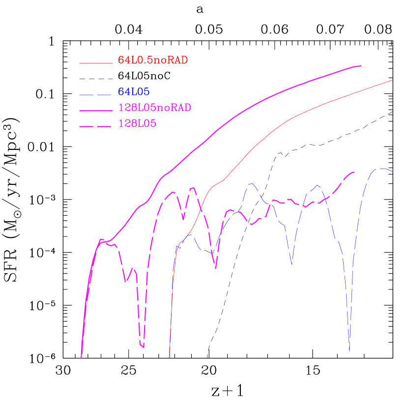
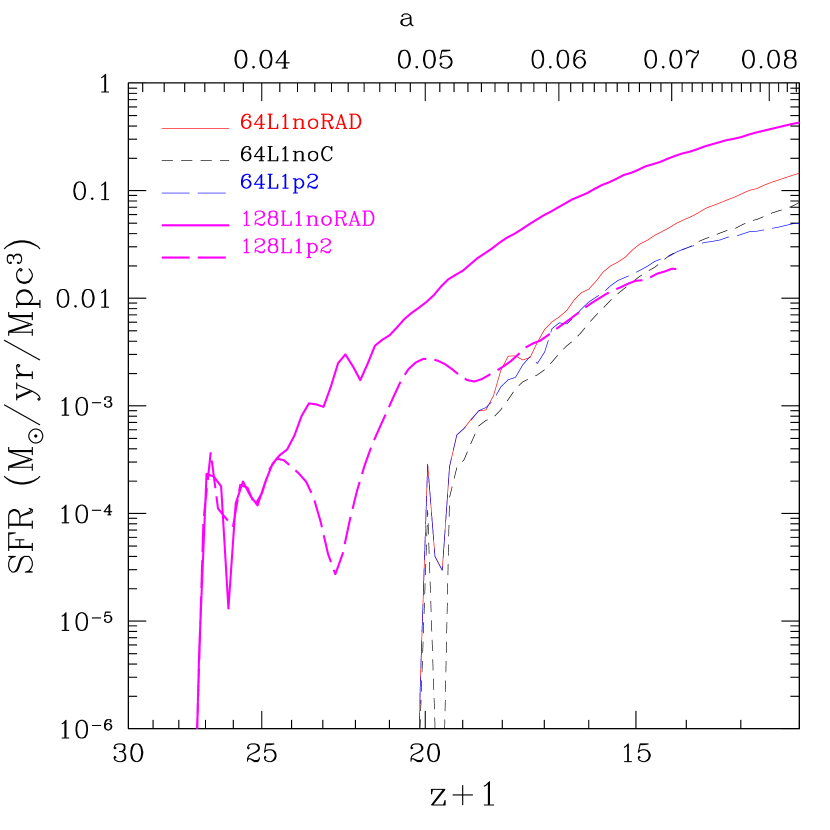
Figure 1: (Left) SFR in 0.5 $h^{-1}$ Mpc box simulations: 64L05noRAD, 64L05noC, 64L05p2, 128L05noRAD, and 128L05p2. The solid lines show simulations without radiative transfer and the long-dashed lines including radiative transfer. The short-dashed line shows a simulation without either radiative transfer or H₂ cooling. (Right) The same as on the left figure but for 1 $h^{-1}$ Mpc box simulations: 64L1noRAD, 64L1noC, 64L1p2, 128L1noRAD, and 128L1p2. The 64L1 simulations have insufficient mass resolution to form “small-halo” objects.

Figure 1 (right) shows the analogous simulations to Figure 1 (left) but for box size $L_{box}=1$ $h^{-1}$ Mpc. The three thin lines show the SFR for the $64^{3}$ box: without radiative transfer (solid), without radiative transfer and H₂ cooling (dashed), and with radiative transfer (long-dashed). The lines are almost indistinguishable, showing that we are forming only “large-halo” objects and that radiative feedback has no effect on their SFR. The DM mass resolution of these simulations, $M_{DM}=3.15\times 10^{5}$ $h^{-1}$ M_⊙, is not sufficient to fully resolve the first “small-halo” objects, with typical masses $M_{DM}\sim 10^{6}-10^{8}$ $h^{-1}$ M_⊙. In Paper I we showed that we need to resolve each object with at least 100 DM particles. The two thick lines show the SFR for the $128^{3}$ boxes without radiative transfer (solid line) and including radiative transfer (long-dashed line). For the simulation with radiative transfer we use the Population II SED and $(\epsilon_{UV}/4\pi)$$\langle f_{esc}\rangle$ $=1.6\times 10^{-5}$. This simulation has mass resolution $M_{DM}=3.94\times 10^{4}$ $h^{-1}$ M_⊙, sufficient to resolve “small-halo” objects, and box size large enough to include the first “large-halo” objects that form at $z\sim 20$. It is shown clearly that the star formation is bursting at $z\lower 2.15277pt\hbox{$\;\buildrel<\over{\sim}\;$}20$ when it is dominated by “small-halo” objects. In this simulation, “large-halo” objects dominate the SFR as soon as they form, producing the continuous star formation mode observed at $z\lower 2.15277pt\hbox{$\;\buildrel>\over{\sim}\;$}20$.

In summary, simulations with mass resolution $M_{DM}<3.15\times 10^{5}$ $h^{-1}$ M_⊙ (such as the 64L1 runs) do not form “small-halo” objects and therefore are not well-suited for this study. On the other hand, if the box is much smaller than 1 $h^{-1}$ Mpc (comoving), the formation of the first “large-halo” objects is delayed considerably. If $L_{box}\geq 1$ $h^{-1}$ Mpc, the first rare massive objects form at $z\sim 20$. From the results of other simulations, not shown here, we have verified that the global SFR does not change if we increase the box size from $L_{box}=1$ $h^{-1}$ Mpc to $L_{box}=8$ $h^{-1}$ Mpc, keeping the mass resolution constant (for redshifts $z>4$). The bursting SF mode of “small-halo” objects is not synchronized throughout the whole universe. Therefore, the strong oscillations of the SFR observed in some of our simulations are an artifact of the finite (actually quite small) size of the simulation box.

In Figure 2 we show a sequence of four 3D-views of the cube for the 128L1p2 run at $z=21.2,17.2,15.7,13.3$. The rendering of the volume is obtained by assigning quadratic opacity to the logarithm of the gas density and linear opacity to the $x_{{\text{H\,\sc ii}}}$ fraction. The colors show the $x_{{\text{H\,\sc ii}}}$ fraction. The cosmological H ii regions expand quickly in the IGM, but when their size becomes on the order of the filamentary structure the expansion stops (in comoving coordinates). The filaments become partially ionized, but the voids remain neutral and reionization cannot occur. At redshift $z\sim 20$ the first “large-halo” objects form. For “large-halo” objects, there is no feedback process that can stop the H ii region from expanding into the low density IGM. Indeed, these H ii regions never stop expanding and eventually reionize the universe. Figure 3 is analogous to the previous figure, but here we show the H₂ abundance for the 64L05p3 run. The H₂ is quickly destroyed in the low density IGM by the build-up of the dissociating background, but new H₂ is continuously reformed in the filaments. Therefore, in the dense regions where galaxy formation occurs, positive feedback dominates over the negative feedback of the dissociating background. In the following sections, we will show that the main mechanisms that regulate galaxy formation of “small-halo” objects are the two positive feedback processes found by Ricotti et al. (2001). In that paper, we discussed the importance of H₂ shells (PFRs: positive feedback regions) that form just in front each Strömgren sphere and inside relic (recombining) H ii regions.

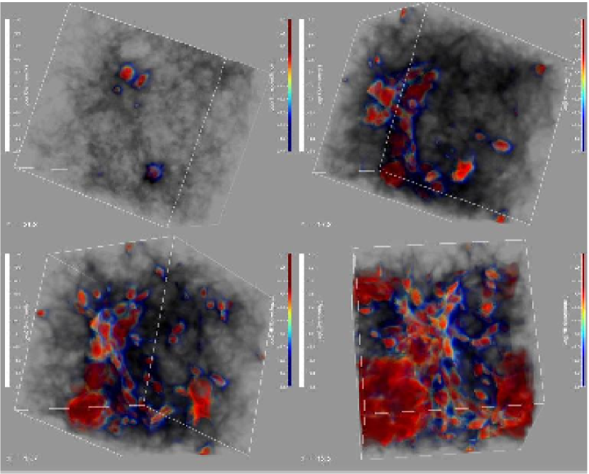
Figure 2: Rendering of the 128L1p2 run at $z=21.2,17.2,15.7,13.3$. The colors code the logarithm of the H ii abundance. “Small-halo” objects produce H ii regions that remain confined in the denser filaments, creating structures that resemble a pearl necklace. At $z=13.3$ the first “large-halo” object produces a large H ii region (big blob on the left of the image) that continues to expand and eventually reionizes the IGM around it.

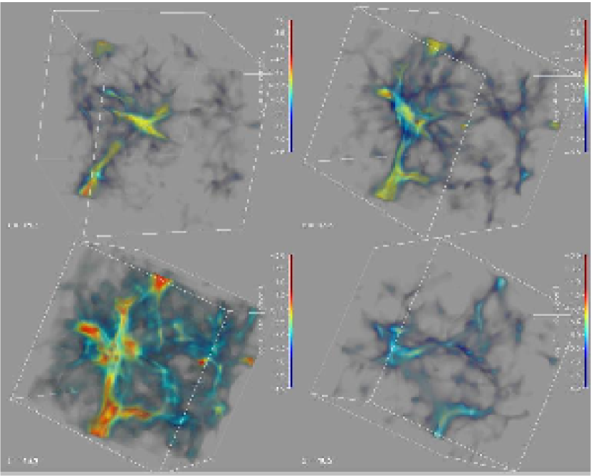
Figure 3: Rendering of the 64L05p3 run at $z=15.7,13.3,12.3,10.2$. The colors code the logarithm of the H₂ abundance.

Since the $128^{3}$ and $256^{3}$ cubes are computationally intensive, in the following three sections (§ 3.1–§ 3.3) we will try to understand the feedback mechanism that regulates the SF of “small-halo” objects using $64^{3}$ cubes with $L_{box}=0.5$ $h^{-1}$ Mpc. We are aware, though, that after $z\sim 20$ we are not properly including the formation of the first “large-halo” objects. In § 3.4 we present the results of our largest simulations that include detailed physics, and realistic values of the free parameters.

3.1 Negative and Positive Feedback

The background intensity in the Lyman-Werner bands determines the redshift at which H₂ is destroyed in the low density IGM. In Figure 4 (top) we show the mean mass- and volume-weighted molecular abundances $\langle x_{H_{2}}\rangle$, $\langle x_{H_{2}^{+}}\rangle$ and $\langle x_{H^{-}}\rangle$ as a function of redshift for the 64L05p2noLW, 64L05p2 and 64L05p3 runs. These runs have the same parameters ($\epsilon_{*}=0.2$, $(\epsilon_{UV}/4\pi)=1.6\times 10^{-5}$, and $\langle f_{esc}\rangle$ $=1$) except for a different flux in the Lyman-Werner bands. The solid line shows the 64L05p2noLW run for which the stars do not emit Lyman-Werner photons. The short-dashed line shows the 64L05p2 run that has a Population II SED, and the long-dashed line shows the 64L05p3 run that has a Population III SED (zero metallicity). The Population II SED emits about 100 times more photons (per M_⊙ of SF) in the Lyman-Werner bands than the Population III SED. Indeed, in the 64L05p2 run, the dissociating background reduces the H₂ abundance in the low-density IGM to a value 1/100 of the H₂ abundance in the 64L05p3 run. In the 64L05p2noLW the H₂ is not destroyed. In Figure 4 (bottom) we show the SFR as a function of redshift for the same simulations. Surprisingly, the SFR does not depend appreciably on the intensity of the dissociating background. It is evident that the destruction of H₂ in the low-density IGM does not affect the global SFR. The only difference in SF history is the run with a Population II SED, which has the higher background in the Lyman-Werner bands. Here, the SFR decreases more than in the other two runs before a new burst occurs. However, on average, also taking into account numerical errors, the SFR is indistinguishable in these three runs.

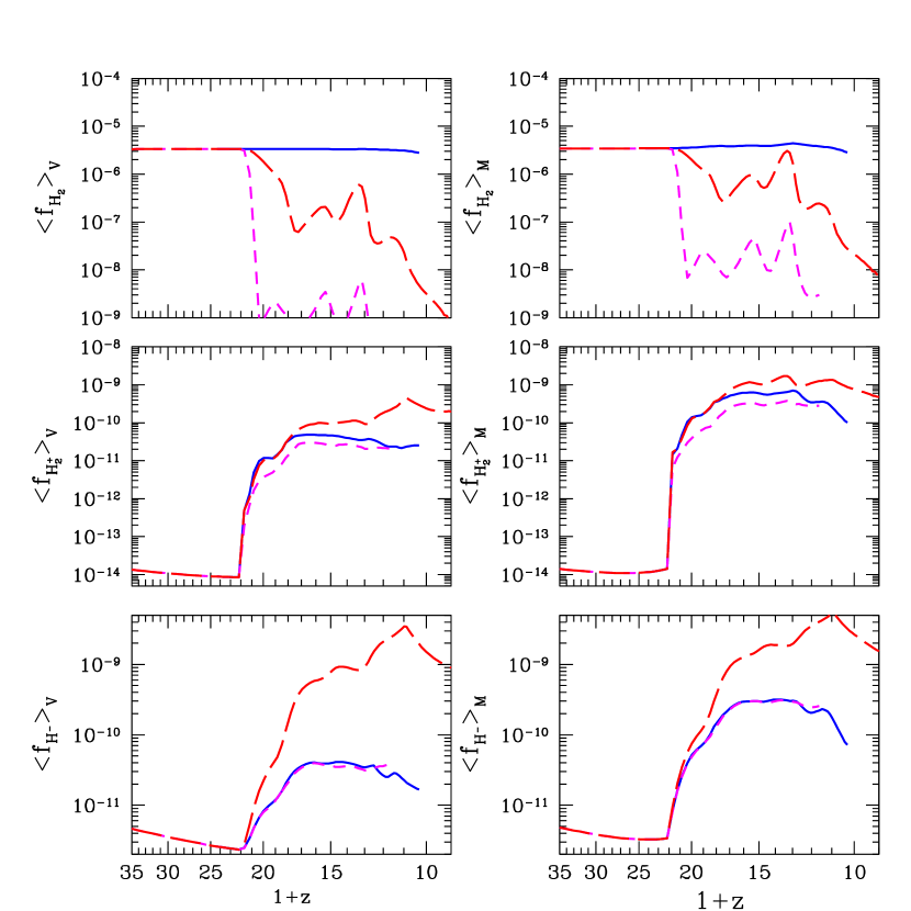
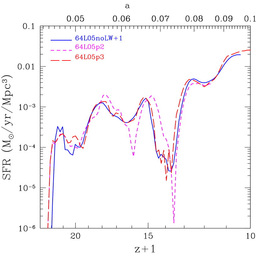
Figure 4: (Top) Species abundances for the 64L05p2noLW (solid line), 64L05p2 (short-dashed line), and 64L05p3 (long-dashed line) runs. These runs have the same parameters ($\epsilon_{*}=0.2$, $(\epsilon_{UV}/4\pi)=1.6\times 10^{-5}$ and $\langle f_{esc}\rangle$ $=1$) except for a different flux in the Lyman-Werner bands. The two top panels show the volume (left) and mass (right) weighted H₂ abundance in the box. The middle and bottom panels show the analogous quantities for H${}_{2}^{+}$ and H^- respectively. (Bottom) The comoving SFR for the same three runs. Despite the fact that the dissociating background flux in these three simulations differs by several orders of magnitude, the SFRs are almost identical.

When the background in the Lyman-Werner bands (averaged over 1000-1100 Å) builds up to $J_{LW}\lower 2.15277pt\hbox{$\;\buildrel>\over{\sim}\;$}10^{-25}$ erg cm^-2 s^-1 Hz^-1 sr^-1 (at $z\sim 20$), it starts to dissociate the H₂ in the IGM. It is evident (Fig. 4) that H₂ is continuously destroyed and reformed. The H₂ abundance peaks are slightly delayed with respect to the SFR minima. Since SF is self-regulated, the dissociating background intensity, after a rapid build-up phase, reaches an almost constant value. Depending on the SED of the sources and $\langle f_{esc}\rangle$, the equilibrium value of the background can be small (e.g., Population III and high $\langle f_{esc}\rangle$) or large (e.g., Population II and small $\langle f_{esc}\rangle$). Consequently, the H₂ abundance in the IGM can assume either a large or small quasi-constant value during the self-regulated SF phase.

In the Population III SED run (long-dashed line), the molecular abundance in the IGM is 100 times higher than in the Population II run, and the mass-weighted abundance becomes $\langle x_{H_{2}}\rangle_{M}\approx 2\times 10^{-6}$ at $z\sim 12$. This means that the positive feedback produced essentially the same mass of H₂ destroyed by negative feedback.

The opacity of the IGM in the Lyman-Werner bands is proportional to the mean H₂ number density. In Figure 5 we show the background specific intensity in $10^{-21}$ erg cm^-2 s^-1 Hz^-1 sr^-1 units, $J_{21}(\nu)$, as a function of frequency for the 64L05p3. We show $J_{21}(\nu)$ at redshift $z=12$ when $\langle x_{H_{2}}\rangle_{M}\sim 2\times 10^{-6}$. In the upper panel, it is interesting to note the importance of the spectral features caused by H i , He i , and He ii Ly$\alpha$ emission lines. The lower panel shows a zoom at the frequencies of the Lyman-Werner bands; the upper (lower) line shows the intensity of the background without (with) line radiative transfer. The H₂ and resonant H i Lyman series line opacities reduce the background intensity by about one order of magnitude.

Figure 5: Background specific intensity in $10^{-21}$ erg cm^-2 s^-1 Hz^-1 sr^-1 units, $J_{21}(\nu)$, as a function of photon energy for the 64L05p3 run (Population III) at $z=12$. The lower panel shows a zoom of the spectrum in the Lyman-Werner bands. In this example, H₂ and H Lyman series line opacities reduce the intensity of the dissociating background in the Lyman-Werner bands by about one order of magnitude (lower line compared to the upper one).

In Figure 6 we show a time sequence of two slices through the most massive object for the 64L05p2 simulation at $z=19.4$ and 18.5. This simulation has $\epsilon_{*}=0.2$, $(\epsilon_{UV}/4\pi)=1.6\times 10^{-5}$, $\langle f_{esc}\rangle$ $=1$, and sources with a Population II SED. Each one of the two panels shows $\log x_{{\text{H\,\sc i}}}$, $\log x_{H_{2}}$, $\log(1+\delta)$ and $\log T$, where $\delta=(\rho-\rho_{0})/\rho_{0}$ is the baryon overdensity with respect to the mean IGM density $\rho_{0}$. At $z=19.4$, the H₂ has its relic abundance everywhere in the IGM except in the dissociation spheres around the first objects, where it is destroyed. At $z=18.5$, the dissociation spheres are still visible, but the UV background starts to dissociate H₂ everywhere in the IGM except in the filaments. Finally, at $z\lower 2.15277pt\hbox{$\;\buildrel<\over{\sim}\;$}18.5$, before the dissociation spheres overlap, the background has destroyed all the relic H₂. The H₂ is still present in the filaments where the gas is partially ionized by stars, and positive feedback dominates. In the analogous simulation, where the sources have a Population III SED, the dissociation spheres never appear around the source. The dissociating background destroys the H₂ in the IGM before the dissociation spheres grow larger than the PFRs. Finally, if $\langle f_{esc}\rangle$ $<1$ and we use a Population II SED for the sources, the dissociation spheres around the sources almost overlap before the background dominates the H₂ dissociation rate. If the dissociating radiation emitted by each source, $S_{LW}$, is large, the dissociating background intensity rises quickly above $J_{LW}\approx 10^{-25}$ erg cm^-2 s^-1 Hz^-1 sr^-1 and the dissociation of H₂ in the IGM happens abruptly. In this case, the dissociation spheres grow fast enough to cover a large volume of the IGM before the contribution of distance sources to the dissociating background builds up substantially. In contrast, if the dissociating radiation emitted by the sources is small, the dissociation spheres grow slowly, while the the additive contribution of distant sources builds up the intensity of the dissociating background more quickly. In this case, the dissociation spheres remain smaller than the PFRs (and therefore invisible) until the dissociating background has destroyed all the H₂ in the IGM.

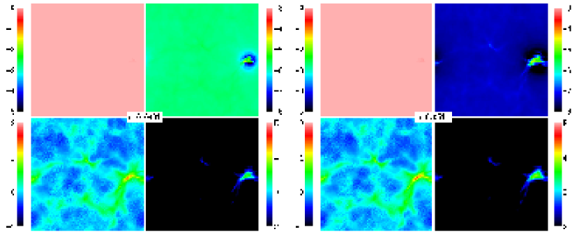
Figure 6: Slices through the most massive object in the simulation of the 64L05p2 box at $z=19.4$ and 18.5. The box size is $L_{box}=0.5$ comoving $h^{-1}$ Mpc. Each one of the two panels shows $\log x_{{\text{H\,\sc i}}}$ (top-left), $\log x_{H_{2}}$ (top-right), $\log(1+\delta)$ (bottom-left) and $\log T$ (bottom-right).

Figure 7 is analogous to Figure 6, except that we now show a zoomed region ($0.125\times 0.125$ $h^{-1}$ Mpc) around the most massive object in the 64L05p3 box. This simulation has $L_{box}=0.5$ $h^{-1}$ Mpc, $\epsilon_{*}=0.2$, $(\epsilon_{UV}/4\pi)=1.6\times 10^{-5}$, $\langle f_{esc}\rangle$ $=1$, and sources with a Population III SED. In this sequence of four slices (at $z=17.3,12.2,11.3$, and 10.2) we recognize the two main processes that create H₂ in the filaments. In the top-left frame at $z=17.3$ we can recognize a PFR as a shell of H₂ surrounding the H ii region that is barely intersected by the slice. In the bottom-left frame ($z=11.3$) two H ii regions are clearly visible. Inside the H ii regions, the H₂ is destroyed. In the bottom-right frame ($z=10.2$) the H ii regions are recombining (demonstrating that the SF is bursting) and new H₂ is being reformed inside the relic H ii regions. A more fine inspection of the time evolution of this slice shows that at least five H ii regions form and recombine between $z=20$ and 10 in this small region of the simulation.

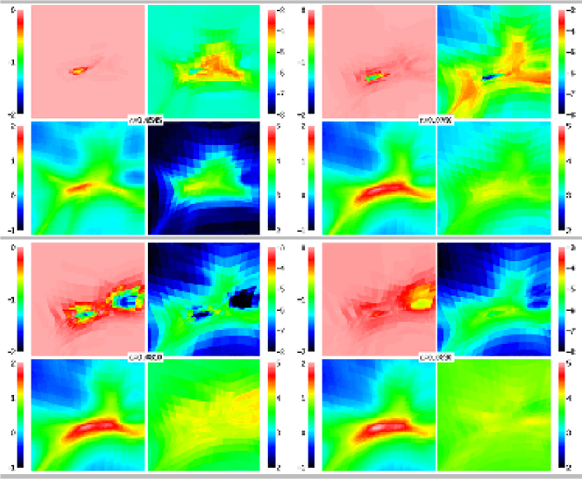
Figure 7: Same as in Figure 6 except for a zoomed region of $0.125^{2}$ $h^{-2}$ Mpc² around the most massive object in the 64L05p3 simulation. In this time sequence of images (top: $z=17.3,12.2$ from left to right; bottom: $z=11.3,10.2$ from left to right) we recognize the two main processes that create H₂ in the filaments: PFRs in front of H ii regions and the reformation of H₂ inside relic H ii regions. The bursting mode of the SF is evident from the continuous formation and recombination of the H ii regions in the time sequence of the slices.

If $\epsilon_{*}(\epsilon_{UV}/4\pi)$$\langle f_{esc}\rangle$ $\ll 3.2\times 10^{-6}$ the SF mode is less violently bursting, and the radiative feedback does not suppress the SFR with respect to the case without radiative transfer. In this case, the positive feedback should be dominated by PFRs preceding the ionization fronts rather than by PFRs inside relic H ii regions. From the inspection of some 3D movies showing the formation of H ii regions, it appears that galaxy formation could be triggered by the presence of neighboring galaxies, in a chain-like process. It is difficult to prove quantitatively this effect, given that galaxies tend to be clustered and, in the early universe, galaxies of very different mass can virialize at the same redshift.

3.2 Self-Regulated Star Formation History

In Figure 8 (left) we compare the SFR of three simulations with $L_{box}=0.5$ $h^{-1}$ Mpc, $(\epsilon_{UV}/4\pi)=1.6\times 10^{-5}$, $\langle f_{esc}\rangle$ $=1$, and a Population III SED (64L05p3, 64L05p3b, 64L05p3c), when we reduce $\epsilon_{*}=0.2$ by a factor of 10 and 100. It appears that the SFR is fairly insensitive to the value of $\epsilon_{*}$ if we consider a realistic range of values $0.2<\epsilon_{*}<0.02$ . As $\epsilon_{*}$ is reduced from 0.2 to 0.02, the oscillations of the global SFR with redshift become more smooth, but its redshift-averaged value gets only a factor of two smaller. When we reduce $\epsilon_{*}$ from 0.02 to 0.002, the global SFR gets a factor of 5 smaller. It is important to note that, when the SFR is dominated by “large-halo” objects, the global SFR is proportional to $\epsilon_{*}$. This result is based on the comparison of several simulations that differ only on the value of $\epsilon_{*}$, some presented here and some presented in Gnedin (2000).

The H i ionizing background, $J_{{\text{H\,\sc i}}}$, has the same behavior as the SFR (i.e., is insensitive to $\epsilon_{*}$). In Figure 8 (right) we show the comoving mean free path of H i ionizing photons $\lambda_{com}$ for the same simulations shown in Figure 8 (left). It is striking that, even if we change $\epsilon_{*}$ by two orders of magnitude, the mean free path of ionizing photons oscillates around a constant value, $\lambda_{com}^{cr}$, shown in the figure by the solid line given by

$$\lambda_{com}^{cr}=0.55~{}h^{-1}~{}{\rm kpc}\left({20\over 1+z}\right)^{2}.$$ (1)

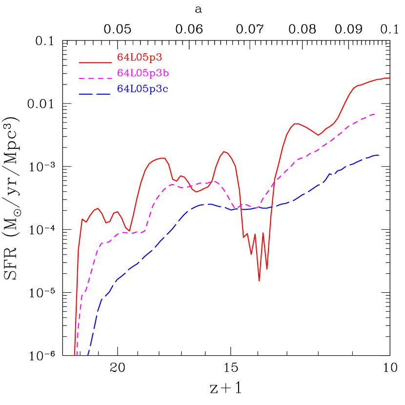
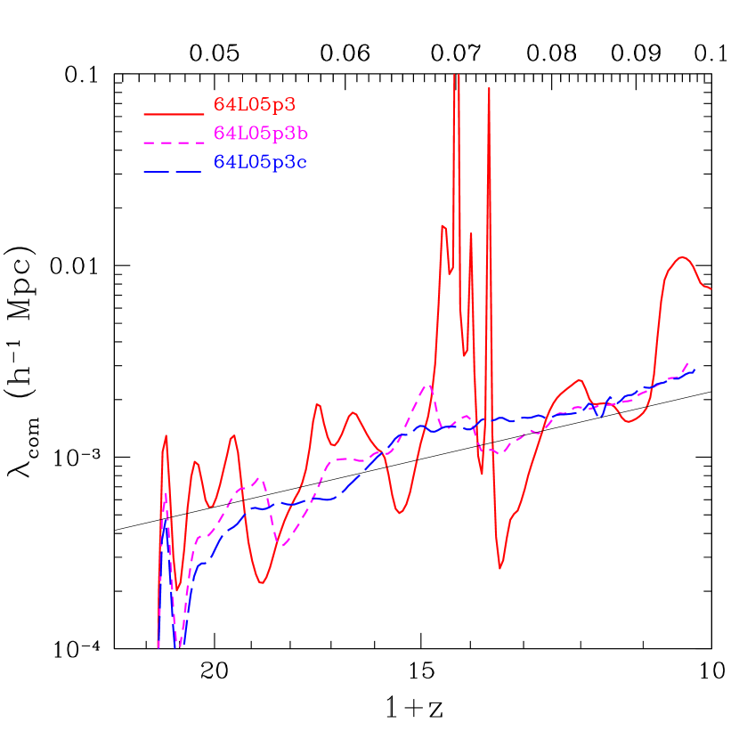
Figure 8: Global SFR (left) and comoving mean free path of H i ionizing photons, $\lambda_{com}$ (right) as a function of redshift for the 64L05p3, 64L05p3b and 64L05p3c runs. The solid, short-dashed, and long-dashed lines have $\epsilon_{*}=0.2,0.02$, and 0.002, respectively. The three simulations have $L_{box}=0.5$ $h^{-1}$ Mpc, $(\epsilon_{UV}/4\pi)=1.6\times 10^{-5}$, $\langle f_{esc}\rangle$ $=1$, and a Population III SED. The global SFR, $J_{{\text{H\,\sc i}}}$, and $\lambda_{com}$, are almost insensitive to $\epsilon_{*}$ for a reasonable range of SFEs ($0.2<\epsilon_{*}<0.02$).

Figure 9 is analogous to Figure 8, but compares simulations varying the value of $\epsilon_{UV}$. The first three runs of the list shown in the figure (thick lines) have the same $\langle f_{esc}\rangle$ $=1$ and $\epsilon_{*}=0.2$, but $\epsilon_{UV}$ is reduced by factors of 10 and 100; the solid, short-dashed and long-dashed lines have $(\epsilon_{UV}/4\pi)=1.6\times 10^{-7},1.6\times 10^{-6}$ and $1.6\times 10^{-5}$, respectively. The last three runs of the list (thin lines), have $\epsilon_{*}=0.02$, and varying $\epsilon_{UV}$; the solid, short-dashed and long-dashed lines have $(\epsilon_{UV}/4\pi)=1.6\times 10^{-6},1.6\times 10^{-5}$ and $1.6\times 10^{-4}$, respectively. Figure 9 (left) shows that the SFR is approximatively inversely proportional to $\epsilon_{UV}$ and insensitive to $\epsilon_{*}$. The inverse proportionality relation is evident when the SF is smooth (compare the thick and thin solid lines). When the SF is bursting the comparison of different simulations is more difficult but the inverse relation appears to hold at least in a limited range of the parameter space. Figure 9 (right) shows that $\lambda_{com}$ is constrained to not exceed a critical value, $\lambda_{com}^{cr}$, shown by the solid line of equation (1). Analogous to $\lambda_{com}$, $J_{{\text{H\,\sc i}}}$ is insensitive to the choice of the free parameters of the simulations. The number of ionizing photons that escape in the IGM is propotional to the parameter combination $\epsilon_{UV}$$\langle f_{esc}\rangle$. Therefore changing $\epsilon_{UV}$ is the same as changing $\langle f_{esc}\rangle$. The only difference is that the SED has more dissociating photons if we reduce $\langle f_{esc}\rangle$ insted of $\epsilon_{UV}$. In § 3.2.1 we show that, unless $\langle f_{esc}\rangle$ is very small, the dissociating radiation does not affect the SFR. In this regime is the value of the parameter combination $\epsilon_{UV}$$\langle f_{esc}\rangle$ that regulates the SFR.

If the product $\epsilon_{*}\epsilon_{UV}$$\langle f_{esc}\rangle$ is large, $\lambda_{com}$ has large oscillations around the critical value, and when the product is small, the oscillations are small. Large oscillations of $\lambda_{com}$ are associated with a strong bursting SF mode. The feedback works in such a way that when $\lambda_{com}$ exceeds the critical value the SF is suppressed, and consequently $\lambda_{com}$ becomes smaller than the critical value. It is easy to show that $\lambda_{com}$ is related to the the H ii region radii. Therefore, the mechanism that self-regulates the SF in “small-halo” objects is related to the size of H ii regions, rather than to the intensity of the dissociating background as previously thought.

Following Gnedin (2000), we can express $\lambda_{com}$ as a function of the mean radius, $R_{\text{H\,\sc ii}}$, of the H ii regions well before the overlap phase. By definition, $\lambda_{com}=[c/\overline{k}(1+z)]$ where $\overline{k}$ is the mean absorption coefficient weighted by the photoionization rate $\Gamma$. The mean optical depth for H i ionizing radiation inside an H ii region is $\langle\tau\rangle=R_{{\text{H\,\sc ii}}}/\lambda_{com}=\langle\sigma_{\text{H\,\sc i}}N_{{\text{H\,\sc i}}}\rangle$, where $\sigma_{\text{H\,\sc i}}$ is the H i ionization cross section and $N_{{\text{H\,\sc i}}}$ is the H i column density of the halo. The H i column density of a virialized halo is

$$N_{{\text{H\,\sc i}}}=x_{\text{H\,\sc i}}n_{vir}R_{vir}\sim 10^{19}~{}{\rm cm}^{-2}\left({1+z\over 20}\right)^{2}.$$

Here $n_{vir}$ is the virial density, $R_{vir}$ is the virial radius of a $M_{DM}\sim 10^{7}$ M_⊙ halo, and $x_{\text{H\,\sc i}}\sim 0.05$ (derived from the simulations) is the hydrogen neutral fraction. Assuming a frequency-averaged value of the H i photoionization cross section $\langle\sigma_{\text{H\,\sc i}}\rangle\sim 10^{-18}$ cm², we have:

$$\lambda_{com}={R^{com}_{\text{H\,\sc ii}}\over\langle\tau\rangle}={R^{com}_{\text{H\,\sc ii}}\over\langle\sigma_{\text{H\,\sc i}}N_{\text{H\,\sc i}}\rangle}\approx 0.1R^{com}_{\text{H\,\sc ii}}[h^{-1}~{}{\rm kpc}]\left({20\over 1+z}\right)^{2},$$ (2)

where $R_{\text{H\,\sc ii}}^{com}$ [$h^{-1}$ kpc ] is the mean free path of ionizing photons. Comparing equation (2) with equation (1), we find that the mean radius of the H ii regions produced by “small-halo” objects is $R_{\text{H\,\sc ii}}^{com}\approx 5$ $h^{-1}$ kpc, about the size of the dense filaments and the virial radii of the halos.

Qualitatively, this result is already evident in Figure 2, which shows that the H ii regions remain confined inside the filaments. The PFRs produced ahead of ionization fronts and the relic H ii regions continuously reform H₂ inside the filaments. The H₂ abundance remains high in the filaments, even when the dissociating background intensity is sufficiently strong to dissociate all the H₂ in the lower-density IGM.

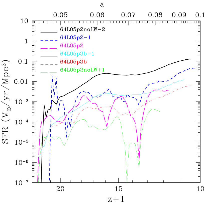
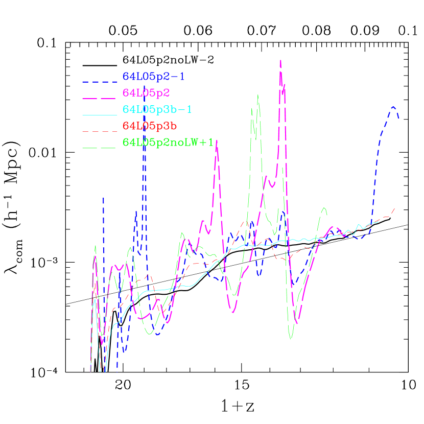
Figure 9: Same as in Figure 8 for the 64L05p2noLW-2, 64L05p2-1, and 64L05p2 runs (thick solid, short-dashed, and long-dashed lines) with $\epsilon_{*}=0.2$, $\langle f_{esc}\rangle$ $=1$, and $(\epsilon_{UV}/4\pi)=1.6\times 10^{-7},1.6\times 10^{-6},1.6\times 10^{-5}$. The thin solid, short-dashed, and long-dashed lines, show the 64L05p3b-1, 64L05p3b, and 64L05p2noLW+1 runs that have $\epsilon_{*}=0.02$, $\langle f_{esc}\rangle$ $=1$, and $(\epsilon_{UV}/4\pi)=1.6\times 10^{-6},1.6\times 10^{-5},1.6\times 10^{-4}$. The three curves in each set of simulations have values of $\epsilon_{UV}$ increased by one order of magnitude. It appears that the SFR is about inversely proportional to $\epsilon_{UV}$ and independent of $\epsilon_{*}$. The comoving mean free path of H i ionizing photons, $\lambda_{com}$, and $J_{{\text{H\,\sc i}}}$, instead, remain constant.

3.2.1 Star Formation History: a Function of $\langle f_{esc}\rangle$

We have seen in the previous section that the SFR is fairly insensitive to $\epsilon_{*}$ over the range $0.02<\epsilon_{*}<0.2$ and inversely proportional to $\epsilon_{UV}$$\langle f_{esc}\rangle$. The free parameter $\epsilon_{UV}$ depends mainly on the stellar IMF and slightly on the stellar metallicity. Assuming a Salpeter IMF we find $(\epsilon_{UV}/4\pi)=1.1\times 10^{-5}$ for a Population II SED and $(\epsilon_{UV}/4\pi)=2.5\times 10^{-5}$ for a Population III SED. Some theoretical arguments suggest that, at high redshift, the IMF could be flatter than a Salpeter IMF. If this is the case, we would have $(\epsilon_{UV}/4\pi)\gg 10^{-5}$. The possibility of having a steeper IMF, and therefore $(\epsilon_{UV}/4\pi)\ll 10^{-5}$, is not supported by any theoretical work or observation.

The value of $\langle f_{esc}\rangle$ is unknown, and has been an argument of debate form many years. In literature, values of $\langle f_{esc}\rangle$ between 0.5 to zero have been proposed. Theoretical work on $\langle f_{esc}\rangle$ for “small-halo” objects at high-redshift (Ricotti & Shull, 2000; Wood & Loeb, 2000) finds that $\langle f_{esc}\rangle$ should be very small ($10^{-2}<$$\langle f_{esc}\rangle$ $<10^{-5}$) and decreasing with increasing halo masses. Observations of $\langle f_{esc}\rangle$ in nearby starburst galaxies find values of $\langle f_{esc}\rangle$ $\lower 2.15277pt\hbox{$\;\buildrel<\over{\sim}\;$}10\%$ (Leitherer et al., 1995; Hurwitz, Jelinsky, & Dixon, 1997; Heckman et al., 2001; Deharveng et al., 2001), in agreement with theoretical studies (Dove, Shull, & Ferrara, 2000). Numerical simulations of the reionization of the IGM usually adopt a value of $\langle f_{esc}\rangle$ $\sim 1$ in order to reionize the universe before redshift $z\sim 6$. A recent study on Lyman break galaxies (Steidel, Pettini, & Adelberger, 2001) agrees with numerical simulations in finding $\langle f_{esc}\rangle$ $\sim 0.5-1$. But there is no observational constraint on the value of $\langle f_{esc}\rangle$ for “small-halo” objects. Reasonably, “small-halo” objects should have smaller $\langle f_{esc}\rangle$ than “large-halo” objects (normal galaxies) since their halos are not collisionally ionized. On the other hand, if a substantial fraction of the ISM is photoevaporated or blown away by stellar winds and SNe, $\langle f_{esc}\rangle$ could be larger. We note that $\langle f_{esc}\rangle$ in this paper is defined as the escape fraction of ionizing photons from the resolution element; therefore it is resolution dependent and generally larger than $\langle f_{esc}\rangle$ from the galactic halos.

In the previous section we showed that, if $(\epsilon_{UV}/4\pi)$$\langle f_{esc}\rangle$ $\lower 2.15277pt\hbox{$\;\buildrel>\over{\sim}\;$}10^{-5}$ and $\epsilon_{*}\lower 2.15277pt\hbox{$\;\buildrel>\over{\sim}\;$}0.02$, the SFR is suppressed by the feedback of ionizing radiation (but not from the dissociating background). Since it is unlikely that $(\epsilon_{UV}/4\pi)<10^{-5}$, the SFR can be increased if $\langle f_{esc}\rangle$ $<1$. As we decrease $\langle f_{esc}\rangle$, the SFR increases almost linearly up to a maximum value determined by the SFR without any feedback. This value is proportional to $\epsilon_{*}$ and to the mass resolution of the simulation. In higher mass resolution simulations, the number of “small-halo” objects that form stars is larger since we resolve many more small-mass objects. We believe that our higher resolution simulation, with $L_{box}=1$ $h^{-1}$ Mpc, $256^{3}$ cells, and mass resolution $M_{DM}=4.93\times 10^{3}$ $h^{-1}$ M_⊙, is close to fully resolving SF for the case without radiative feedback (we need to resolve each halo with about 100 DM particles).

Clearly, if $\langle f_{esc}\rangle$ $=0$, there should be no positive feedback, but only the negative feedback of the dissociating background, which should determine the SFR. Indeed, if we decrease the value of $\langle f_{esc}\rangle$ below a critical value, the SFR, after reaching the maximum, starts decreasing. This effect is shown in Figure 10 (left), where the lines show simulations with $\epsilon_{*}=0.2$, Population II SED and $\langle f_{esc}\rangle$ $=1,0.1,0.01,10^{-3},10^{-5}$ (64L05p2, 64L05p2-1f, 64L05p2-2f, 64L05p2-3f and 64L05p2-5f runs respectivelly). At $z=15.5$, in the simulation with $\langle f_{esc}\rangle$ $=0.01$, the intensity of the dissociating background is about $J_{LW}\sim 5\times 10^{-21}$ erg cm^-2 s^-1 Hz^-1 sr^-1. The value of $J_{LW}$ is high enough to decrease the SFR with respect to the case without radiative transfer by about a factor of two. In Figure 10 (right), we show the different importance of the dissociating radiation feedback for a Population II and a Population III SED. All the simulations in Figure 10 (right) have $\langle f_{esc}\rangle$ $=0.01$ (runs 64L05p2-2f, 64L05p3-2f, 64L05p2-2fa and 64L05p3-2fa in Table 1).

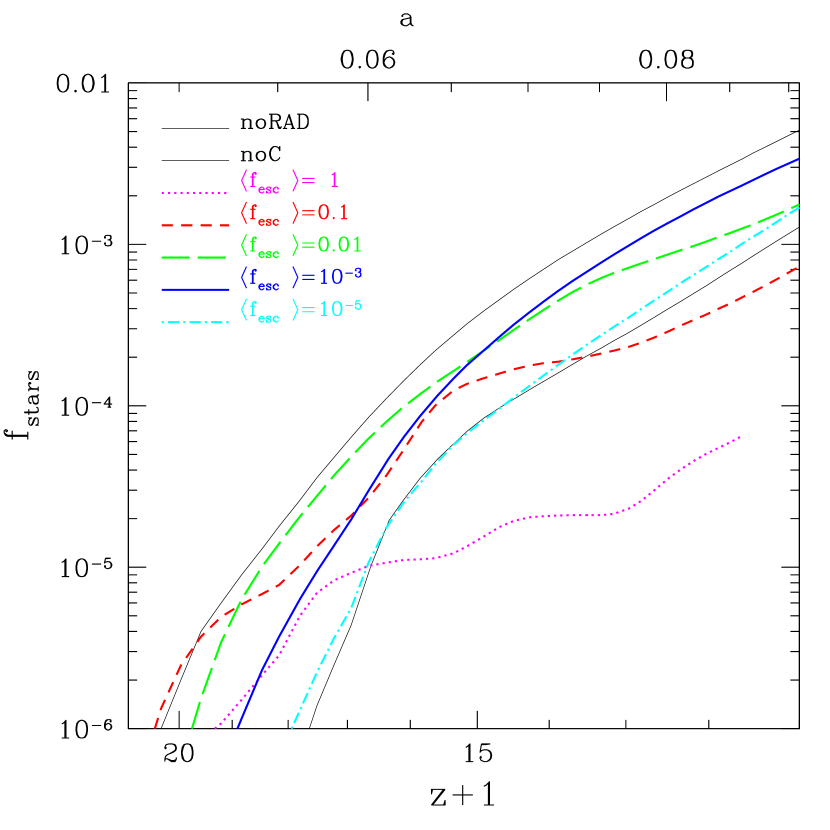
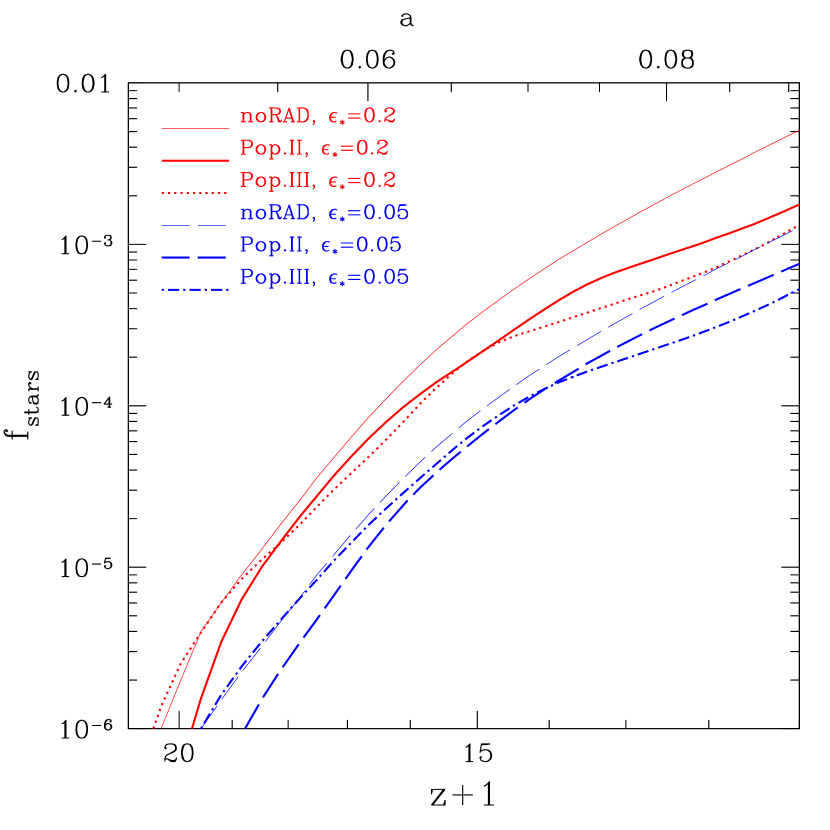
Figure 10: Stellar fraction, $f_{star}$, as a function of redshift. (Left) The two thin solid lines show $f_{star}$ for a simulation without radiative transfer and without either radiative transfer or H₂ cooling. The thick lines show simulations with $\langle f_{esc}\rangle$ $=1,0.1,0.01,10^{-3},10^{-5}$ as shown in the label. Positive feedback increases the SFR as we decrease $\langle f_{esc}\rangle$ from 1 to about $10^{-3}$. If $\langle f_{esc}\rangle$ $\lower 2.15277pt\hbox{$\;\buildrel<\over{\sim}\;$}10^{-3}$ the dissociating background is effective in suppressing the SF. (Right) The thin solid line shows $f_{star}$ for a simulation without radiative transfer and $\epsilon_{*}=0.2$; the thick solid and dotted lines show simulations with $\langle f_{esc}\rangle$ $=0.01$, and $\epsilon_{*}=0.2$, using a Population II or Population III SED, respectively. The thin dashed, thick dashed, and thick dot-dashed lines are analogous to the thin solid, thick solid, and thick dotted lines, but for $\epsilon_{*}=0.05$.

The effect of decreasing excessively the value of $\langle f_{esc}\rangle$ on the SFR is twofold: (i) it reduces the positive feedback of the EUV radiation; and (ii) it increases the relative importance of the dissociating radiation over the ionizing radiation by modifying the SED, $g_{\nu}$. The negative feedback of the dissociating background starts to affect the SFR, depending on magnitude of the jump, $\beta$, at the Lyc frequency of the SED, and the magnitude of the positive feedback. The jump $\beta$ is inversely proportional to $\langle f_{esc}\rangle$ and depends on the SED (intrinsic jump). For the same $\langle f_{esc}\rangle$, the Population II SED produces a jump 10 times larger than the Population III SED. We find that, if $0.02\lower 2.15277pt\hbox{$\;\buildrel<\over{\sim}\;$}\epsilon_{*}\lower 2.15277pt\hbox{$\;\buildrel<\over{\sim}\;$}0.2$, the critical value for which the negative feedback of the dissociating background starts to affect the SFR is $\langle f_{esc}\rangle$ ${}^{cr}\lower 2.15277pt\hbox{$\;\buildrel<\over{\sim}\;$}10^{-2}$ for the Population II SED, and $\langle f_{esc}\rangle$ ${}^{cr}\lower 2.15277pt\hbox{$\;\buildrel<\over{\sim}\;$}10^{-3}$ for the Population III SED.

In Figure 11 we show a case where the positive feedback produces enhanced global SFR with respect to the case without radiative feedback. The simulation (thick dashed line) has $\epsilon_{*}=0.02$, $\langle f_{esc}\rangle$ $=1$, $(\epsilon_{UV}/4\pi)=1.6\times 10^{-9}$, and a Population III SED (64L05p3b-3 run). The thin solid line shows the analogous simulation without radiative transfer. The thick dashed line shows a simulation with the same value of the parameter combination $\epsilon_{UV}$$\langle f_{esc}\rangle$ as the 64L05p3b-3 run, but with Salpeter IMF ($(\epsilon_{UV}/4\pi)=1.6\times 10^{-5}$) and $\langle f_{esc}\rangle$ $=10^{-3}$. The SFR in these two simulations should be identical, since it depends on the parameter combination $\epsilon_{UV}$$\langle f_{esc}\rangle$. Instead, the negative feedback of the dissociating background reduces the SFR by a factor of three with respect to the 64L05p3b-3 run. The dissociating background in the simulation with $\langle f_{esc}\rangle$ $=10^{-3}$ is three orders of magnitude higher ($J_{LW}\sim 0.5\times 10^{-21}$ erg cm^-2 s^-1 Hz^-1 sr^-1 at $z=11.5$) than in the simulation with $\langle f_{esc}\rangle$ $=1$.

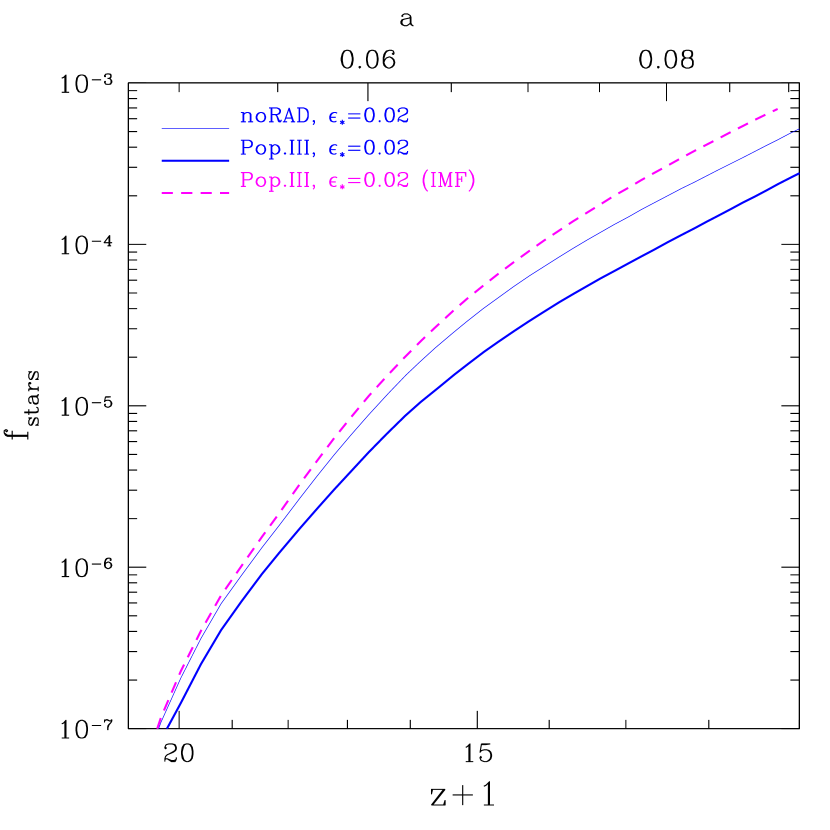
Figure 11: Stellar fraction, $f_{star}$ as a function of redshift for the 64L05noRAD (without radiative transfer, thin solid line), 64L05p3b-3 (thick solid line), and 64L05p3b-3n (thick dashed line) runs. The simulations have $L_{box}=0.5$ $h^{-1}$ Mpc, $\epsilon_{*}=0.02$, and a Population III SED. The 64L05p3b-3 has $\langle f_{esc}\rangle$ $=10^{-3}$ and $(\epsilon_{UV}/4\pi)=1.6\times 10^{-6}$. The 64L05p3b-3n run has $\langle f_{esc}\rangle$ $=1$ and $(\epsilon_{UV}/4\pi)=1.6\times 10^{-9}$ (flat IMF). The dissociating background is three orders of magnitude higher in the run with $\langle f_{esc}\rangle$ $=10^{-3}$.

The simulations presented in this section have mass resolution $M_{DM}=3.94\times 10^{4}$ $h^{-1}$ M_⊙. The global SFR (without radiative feedback) is underestimated because we do not resolve the lowest mass objects that can form stars. Higher resolution simulations could produce an enhanced SFR with respect to the case without including any feedback. Indeed, positive feedback can trigger SF in halos with a mass smaller than the minimum mass derived in the absence of feedback. Theoretically, the lower limit for the DM mass of an object that could form stars is determined by the filtering mass that is $M_{F}\sim 10^{5}-10^{6}$ $h^{-1}$ M_⊙ in the redshift range $20<z<100$. In objects with DM masses smaller than $M_{F}$, the baryons cannot virialize.

3.2.2 How does the Self-Regulation Work?

Summarizing, the feedback prevents the size of H ii regions from exceeding $R_{{\text{H\,\sc ii}}}^{com}\approx 5$ $h^{-1}$ kpc (about the size of the dense filaments). Indeed when the H ii regions get bigger than the filaments molecular hydrogen is destroyed and the SF is suppressed. On the contrary, when the H ii regions are smaller than the filaments or when they recombine after a burst of SF, the dense filaments are only partially ionized and the formation rate of molecular hydrogen is maximized. Since galaxy formation takes place only in overdense regions, the SF is self-regulated to maximize H₂ formation in the filaments. Thus, the volume filling factor of the H ii regions remains small. As a result, “small-halo” objects cannot reionize the universe. Molecular hydrogen is continuously reformed, in shells preceding the H ii regions and in shells inside relic H ii regions, the PFRs found by Ricotti et al. (2001). SF is bursting, since it is self-regulated by the two above-mentioned feedback mechanisms. The SFR does not depend on $\epsilon_{*}$ or on the source SED, but only on $\langle f_{esc}\rangle$ and the IMF through $\epsilon_{UV}$. If $\epsilon_{UV}$$\langle f_{esc}\rangle$ is small, the SFR is high, and vice versa. Indeed, if few ionizing photons (per each baryon converted into stars) escape from the halo, more stars have to be formed in order to produce H ii regions of the size of the filaments. If the product $\epsilon_{*}\epsilon_{UV}$$\langle f_{esc}\rangle$ is large, the SF burst is so fast that H ii regions will expand outside the filaments before recombining. This produces a temporary halt in the global SF, which appears as a sequence of strong bursts. It is fascinating that the SF history of “small-halo” objects depends primarily on a single parameter, $\epsilon_{UV}$$\langle f_{esc}\rangle$. This happens because the feedback mechanism acts on a cosmological (rather than galactic) scale. We notice, though, that $\langle f_{esc}\rangle$ should depend slightly on $\epsilon_{*}$ (Ricotti & Shull, 2000).

In Figure 12 we show a sketch of the relative importance of positive and negative feedback from EUV (ionizing) and FUV (dissociating) radiation on the SFR. The thick and the thin solid curves show the SFR with and without radiative transfer, respectively, for a simulation with $\epsilon_{*}=0.2$, Population II SED ($(\epsilon_{UV}/4\pi)=1.1\times 10^{-5}$), and $\langle f_{esc}\rangle$ $=0.01$. Without radiative feedback, the SFR is proportional to $\epsilon_{*}$. Therefore, for a simulation with $\epsilon_{*}=0.02$, for instance, the SFR shown by the thin solid curve would be a factor of ten smaller. The solid line shows the region where the positive feedback from EUV radiation is maximum. The SFR of this line is inversely proportional to the parameter combination $\epsilon_{UV}$$\langle f_{esc}\rangle$. Above the solid line, we have increasing negative feedback from EUV radiation (H ii regions become larger than the filaments), and below the line the positive feedback from EUV radiation becomes increasingly weak. If the parameter combination $\epsilon_{*}\epsilon_{UV}$$\langle f_{esc}\rangle$ $\lower 2.15277pt\hbox{$\;\buildrel<\over{\sim}\;$}10^{-6}-10^{-7}$, the SFR is not suppressed by EUV radiative feedback (in this case the solid line lies above the thin solid curve). When the flux of ionizing photons in the filaments is too small, either because $\langle f_{esc}\rangle$ is small or because of a low SFR, positive feedback effects are weak. The negative feedback of the dissociating background becomes, therefore, important. Below the thin dashed line, the negative feedback from FUV radiation starts to dominate the positive feedback from EUV radiation. The region between the solid and dashed lines is where the positive feedback dominates over negative feedback, and its size is inversely proportional to the jump $\beta$ at the Lyc of the source SED. The effect of the FUV negative feedback is usually to delay SF at high-redshift, when the SFR, and therefore the ionizing photon flux is lower. At higher redshift, as the number of “small-halo” objects increases, the positive feedback dominates and the SFR becomes self-regulated by the EUV radiation. In the extreme case of a very small $\langle f_{esc}\rangle$ ($\langle f_{esc}\rangle$ $\lower 2.15277pt\hbox{$\;\buildrel<\over{\sim}\;$}10^{-3}$ for a Population II SED, and $\langle f_{esc}\rangle$ $\lower 2.15277pt\hbox{$\;\buildrel<\over{\sim}\;$}10^{-4}$ for a Population III SED), the negative feedback of the dissociating background can suppress “small-halo” object formation.

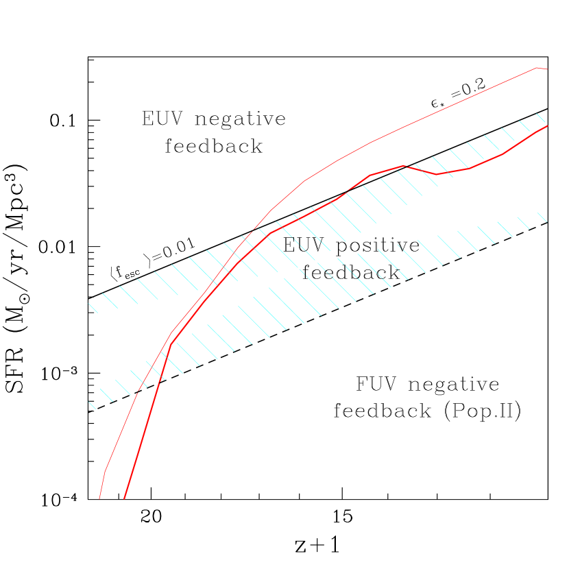
Figure 12: Sketch showing the relative importance of positive and negative feedback from EUV (ionizing) and FUV (dissociating) radiation on the SFR. The thick and thin solid lines show the SFR with and without radiative feedback, respectively (both for $\epsilon_{*}=0.2$ and $\langle f_{esc}\rangle$ $=0.01$). The shaded strip is where positive feedback dominates. Above the strip, the SF is suppressed by feedback from ionizing (EUV) radiation, and below from the feedback from H₂ dissociating radiation.

3.3 Metal Enrichment of the IGM

Metals are produced by the same massive stars that produce ionizing radiation. Understanding the metal enrichment of the low density IGM is a challenging task. Observational constraints from the metallicity evolution of the Ly$\alpha$ forest allow us to test the models. In Figure 13 we show a 3D rendering of the IGM metallicity (in solar units) for the 64L05p3 run ($L_{box}=0.5$ $h^{-1}$ Mpc, $\epsilon_{*}=0.2$, $(\epsilon_{UV}/4\pi)=1.6\times 10^{-5}$, $\langle f_{esc}\rangle$ $=1$, and a Population III SED). The opacity and the color coding are proportional to the logarithm of the metallicity ($Z/Z_{\odot}$). The comoving volume filling factor of the metal enriched gas increases quickly at high-redshift and slows down as the redshift decreases.

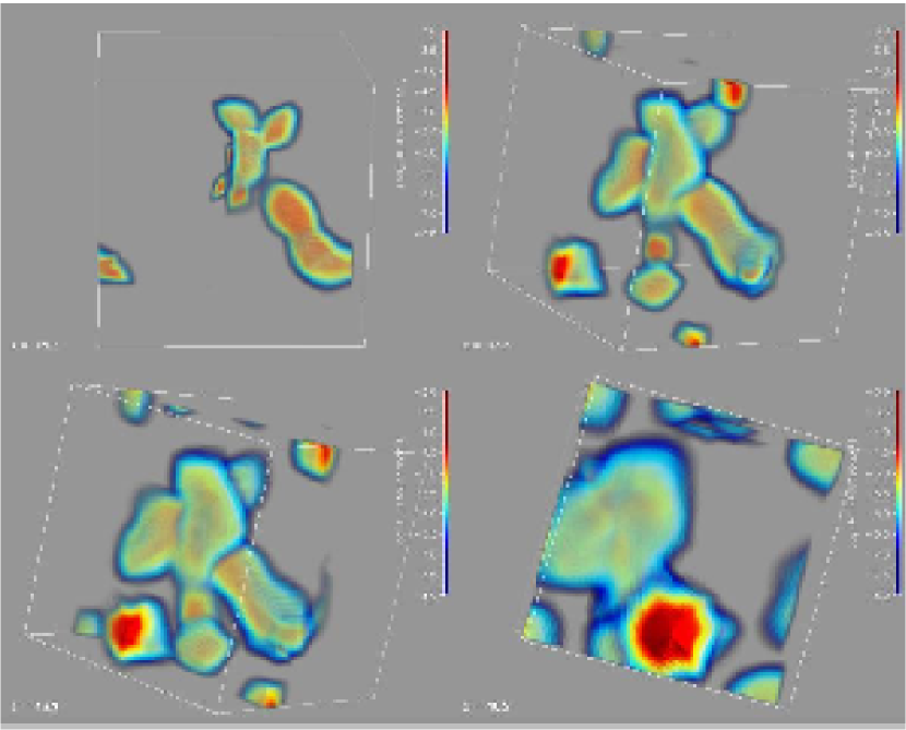
Figure 13: 3D rendering of the logarithm of the IGM metallicity (in solar units) for the 64L05p3 run. The four cubes show the time evolution of the volume filling factor of metal-enriched gas at $z=15.7,13.3,12.3$, and 10.2.

In Figure 14 (left) we show the ratio $\langle Z/Z_{\odot}\rangle_{V}/\langle Z/Z_{\odot}\rangle_{M}$ of the volume- to mass-weighted mean metallicities as a function of redshift. This ratio is proportional to the filling factor of the metal enriched gas. The solid line shows the 64L05noRAD run ($L_{box}=0.5$ $h^{-1}$ Mpc, $\epsilon_{*}=0.2$, $(\epsilon_{UV}/4\pi)=1.6\times 10^{-5}$, without radiative transfer). The dotted, dashed, and long-dashed lines show simulations with $\langle f_{esc}\rangle$ $=1$ and an increasing value of the parameter combination $\epsilon_{*}(\epsilon_{UV}/4\pi)$$\langle f_{esc}\rangle$ $=3.2\times 10^{-8},3.2\times 10^{-7}$, and $3.2\times 10^{-6}$. We remind the reader that, if the value of this parameter combination is high, the global SF, $J_{{\text{H\,\sc i}}}$, and $\lambda_{com}$, are strongly oscillating (bursty SF). The filling factor of metal-enriched gas is larger in the simulations with strongly bursting SF. This suggests that photo-evaporation of high-redshift “small-halo” galaxies is an important mechanism for transporting metals in the low density IGM (voids).

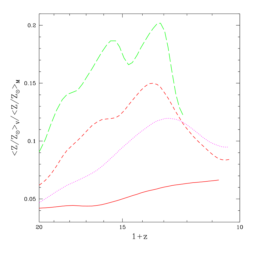
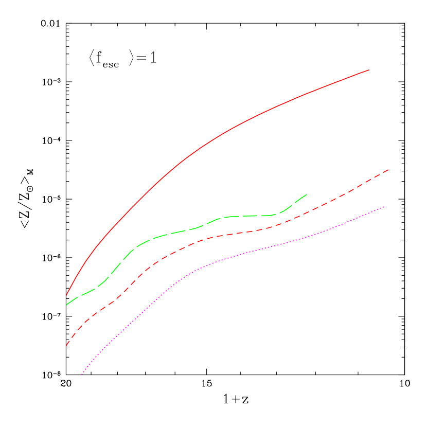
Figure 14: (Left) Ratio of the volume- and mass-weighted mean metallicities, $\langle Z/Z_{\odot}\rangle_{V}/\langle Z/Z_{\odot}\rangle_{M}$, as a function of redshift for the 64L05noRAD (solid), 64L05p2-2 (dotted), 64L05p3b (dashed), and 64L05p2noLW+1 (long-dashed) runs. This ratio is proportional to the volume filling factor of the metal enriched gas. The lines, from the bottom to the top, have an increasingly bursting SF mode. The SF bursts are stronger when the parameter combination $\epsilon_{*}\epsilon_{UV}$$\langle f_{esc}\rangle$ is large. (Right) Mass-weighted mean metallicity, $\langle Z/Z_{\odot}\rangle_{M}$, as a function of redshift.

Figure 14 (right) shows the mass-weighted metallicity $\langle Z/Z_{\odot}\rangle_{M}$ for the four simulations in Figure 14 (left). It can be easily shown that $\langle Z/Z_{\odot}\rangle_{M}\propto\epsilon_{UV}f_{star}$, where $f_{star}$ is the mass fraction in stars and $\epsilon_{UV}$ is the energy in ionizing photons per rest mass energy of H atoms ($m_{H}c^{2}$) transformed into stars (the number of ionizing photons emitted by a population of stars is proportional to the number of heavy elements released in the ISM). The parameter $\epsilon_{UV}$ depends on the IMF and stellar metallicity. If the feedback of the EUV radiation regulates the SFR, we have $f_{star}\propto(\epsilon_{UV}\langle f_{esc}\rangle)^{-1}$. In this case, we expect $\langle Z/Z_{\odot}\rangle_{M}\propto$$\langle f_{esc}\rangle$ ^-1, independent of the stellar metallicity and IMF. We conclude that, while the SFR and $f_{stars}$ is inversely proportional to the parameter combination $\epsilon_{UV}$$\langle f_{esc}\rangle$, the mass of metals produced by “small-halo” depends only on $\langle f_{esc}\rangle$. In Figure 14 we have used $\langle f_{esc}\rangle$ $=1$.

3.4 Realistic Scenarios of Cosmic Evolution during the “Dark Ages”

In this section we show the evolution of the global properties of the universe in our three most realistic simulations: the 128L1p2, 128L1p2-2 and 256L1p3 runs. The mass resolution ($M_{DM}=4.93\times 10^{3}$ $h^{-1}$ M_⊙ for the $256^{3}$ and $3.94\times 10^{4}$ $h^{-1}$ M_⊙ for the $128^{3}$ runs) and box size, $L_{box}=1$ $h^{-1}$ Mpc, of these simulations is sufficiently large to resolve the formation of the first “small-halo” and “large-halo” objects. In particular, the 128L1p2-2 and 256L1p3 simulations include the effects of secondary electrons and the SED modification caused by assuming realistic values of $\langle f_{esc}\rangle$. We have $\langle f_{esc}\rangle$ $=0.1$, $\epsilon_{*}=0.1$, and metal-free SED ($(\epsilon_{UV}/4\pi)=2.5\times 10^{-5}$) for the 256L1p3 run. For the 128L1p2-2 run we assume $\langle f_{esc}\rangle$ $=0.01$, $\epsilon_{*}=0.05$ and $Z=0.05Z_{\odot}$ Population II SED ($(\epsilon_{UV}/4\pi)=1.1\times 10^{-5}$). The 128L1p2 run has $\langle f_{esc}\rangle$ $=1$, $\epsilon_{*}=0.2$, $(\epsilon_{UV}/4\pi)=1.6\times 10^{-5}$ and Population II SED. We believe that the $256^{3}$ run is very close to the limit of numerical convergence. Finally, the formal spatial resolution is $156$ $h^{-1}$ pc comoving [$B_{*}=25$ is the parameter that regulates the maximum deformation of the Lagrangian mesh: the spatial resolution is $\sim L_{box}/(N_{box}B_{*})$] in the 256L1p3 run, $488$ $h^{-1}$ pc comoving ($B_{*}=16$) in the 128L1p2-2 run, and $781$ $h^{-1}$ pc comoving ($B_{*}=10$) in the 128L1p2 run. To give a better idea of the scales resolved by the simulations, we remind the reader that the comoving core radius of a just-virialized DM halo of mass $M_{DM}$ is $R_{c}\approx 300~{}{\rm pc}(M_{DM}/10^{6}M_{\odot})^{1/3}$ (we have assumed a halo concentration parameter $c=R_{vir}/R_{c}=10$). We refer the reader to Paper I for details on the physics included in the code and in our convergence studies.

The thick solid lines in Figure 15 show the comoving SFR and fraction of baryons in stars, $f_{star}$, as a function of redshift for the 256L1p3 run (left panels), 128L1p2-2 run (center panels) and 128L1p2 run (right panels). As a comparison we plot the same runs without radiative transfer (dashed lines) and the 64L1noC run ($64^{3}$ cells and $L_{box}=1$ $h^{-1}$ Mpc), excluding both radiative transfer and H₂ cooling (thin solid lines). Therefore, thin solid lines show the contribution to the global SFR of “large-halo” objects only, and the dashed lines show the SFR of “small-halo” and “large-halo” objects without any feedback effect. The main result shown in this figure is that “small-halo” objects are an extremely important (or dominant) fraction of the galaxies at least until redshift $z\sim 10$. Contrary to what is widely believed, their formation is not severely suppressed by the dissociating background. We showed in § 3.1 that the dissociating background has little influence in determining the SF history. In § 3.2 we demonstrated that the mass fraction of “small-halo” objects formed depends, instead, only on the value of $\langle f_{esc}\rangle$ and the stellar IMF.

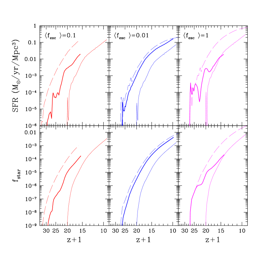
Figure 15: The thick solid lines show the SFR (top panels) and fraction of baryons in stars, $f_{star}$ (bottom panels), as a function of redshift for the 256L1p3 (left panels), 128L1p2-2 (center panels) and 128L1p2 (right panels) simulations. The box size is 1 $h^{-1}$ Mpc comoving. The 256L1p3 run has a Population III SED, $\langle f_{esc}\rangle$ $=0.1$ and $\epsilon_{*}=0.1$; the 128L1p2-2 run has Population II SED, $\langle f_{esc}\rangle$ $=0.01$ and $\epsilon_{*}=0.05$, and the 128L1p2 run has Population II SED, $\langle f_{esc}\rangle$ $=1$ and $\epsilon_{*}=0.2$. The thin dashed lines show the same simulations, without radiative transfer, and the thin solid lines excluding both radiative transfer and H₂ cooling (i.e., the contribution of “large-halo” objects).

The two panels on the left of Figure 15 show the SFR and $f_{star}$ for the $256^{3}$ cells simulation which has $\langle f_{esc}\rangle$ $=0.1$; in this simulation the first stars form at $z=30$. At $z=15$ the fraction of stars in “small-halo” objects is $f_{star}\simeq 2\times 10^{-4}$, about 5 times the mass of stars in “large-halo” objects. The radiative feedback has reduced $f_{star}$ by a factor of 10. Note that $f_{star}$ for “large-halo” objects (thin solid line) and for “small-halo” objects without feedback (thin long-dashed line) scales with $\epsilon_{*}$. The fraction of baryons transformed into stars of “small-halo” objects, including radiative feedback effects, does not depend on $\epsilon_{*}$ as long as it is smaller than the the value without radiative transfer. Since, for “large-halo” objects, $f_{star}\propto\epsilon_{*}$, the relative importance of “small-halo” to “large-halo” objects is inversely proportional to $\epsilon_{*}$ (which here is 0.1). For instance, if we had chosen $\epsilon_{*}<0.1$ for this simulation, $f_{star}$ of “small-halo” objects would have been as large as 50 times $f_{star}$ of “large-halo” objects at $z=15$, and the radiative feedback would have suppressed the SF by only a small factor.

We show an example of such a case in the two central panels of Figure 15. In this $128^{3}$ simulation we use $\langle f_{esc}\rangle$ $=0.01$ and $\epsilon_{*}=0.05$. Here, the first stars form at $z=26$ because of the lower mass resolution. Radiative feedback suppresses the SFR only by a factor of 2. At $z=15$, $f_{star}\simeq 3\times 10^{-4}$, and the contribution of “small-halo” objects to star formation is about 10 times the contribution of “large-halo” objects. At $z=10$, “small-halo” objects still dominate $f_{star}$ by a factor of 3. Note that in this simulation the dissociating background intensity is very high and, as shown by the short-dashed lines in Figure 16, the H^- and H₂ abundances in the IGM are extremely small ($\sim 10^{-12}$ relative to H).

The two panels on the right show the SFR and $f_{star}$ for the $128^{3}$ simulation, which has $\langle f_{esc}\rangle$ $=1$ and $\epsilon_{*}=0.2$. At $z=15$, the fraction of stars in “small-halo” objects is $f_{star}\simeq 2\times 10^{-5}$, about 1/5 the mass of stars in “large-halo” objects. The radiative feedback has reduced $f_{star}$ by a factor of 100.

In Figure 16 we show the mass- and volume-weighted mean molecular abundances $\langle x_{H_{2}}\rangle$, $\langle x_{H_{2}^{+}}\rangle$ and $\langle x_{H^{-}}\rangle$ as a function of redshift for the three simulations with radiative transfer shown in Figure 15. The volume-weighted abundances are about two orders of magnitude smaller than the mass-weighted abundance. This shows that H₂ is much more abundant in dense regions. The dissociating background destroys the H₂ in the low-density IGM in the redshift range $20<z<25$, depending on the choice of the free parameters in the simulation. In the dense regions, the production/destruction of H₂ sets its abundance to a quasi-constant value that depends on the SED of the sources. At redshift $z\sim 15$, the abundance of H^-, the main catalyst for H₂ production, reaches its maximum value and starts to decrease. Consequently, the H₂ abundance also decreases after $z\sim 15$.

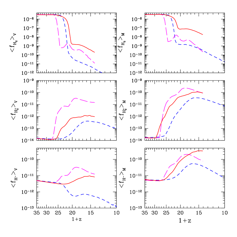
Figure 16: Mass- and volume-weighted molecular abundances $\langle x_{H_{2}}\rangle$, $\langle x_{H_{2}^{+}}\rangle$ and $\langle x_{H^{-}}\rangle$ for the three runs from Figure 15. The solid lines show the 256L1p3 run ($\langle f_{esc}\rangle$ $=0.1$ and $\epsilon_{*}=0.1$), the short-dashed lines show the 128L1p2-2 run ($\langle f_{esc}\rangle$ $=0.01$ and $\epsilon_{*}=0.05$), and the long-dashed lines show the 128L1p2 run ($\langle f_{esc}\rangle$ $=1$ and $\epsilon_{*}=0.2$). The drops in H₂ abundance, while H${}_{2}^{+}$ and H^- are still high, are due to the rising flux of the dissociating radiation.

Figure 17 is analogous to Figure 16, but here we show the mass- and volume-weighted ionized H and He mean abundances $\langle x_{{\text{H\,\sc ii}}}\rangle$, $\langle x_{{\text{He\,\sc ii}}}\rangle$, $\langle x_{{\text{He\,\sc iii}}}\rangle$ (top), and the metallicity $\langle Z/Z_{\odot}\rangle$ and temperature $\langle T\rangle$ (bottom). If reionization takes place at redshift $z\sim 6$, as recent high-redshift quasar observations seem to suggest (Becker et al., 2001; Djorgovski et al., 2001), the run shown by the long-dashed line reionizes the universe too early, while the run shown by the short-dashed line reionizes the universe too late. This observation does not constrain the value of $\langle f_{esc}\rangle$ or $\epsilon_{*}$ for “small-halo” objects, since we expect that $\langle f_{esc}\rangle$, at least, will vary as a function of redshift. In this paper, we assume for simplicity that $\langle f_{esc}\rangle$, $\epsilon_{*}$, $\epsilon_{UV}$, and $g_{\nu}$ are constants.

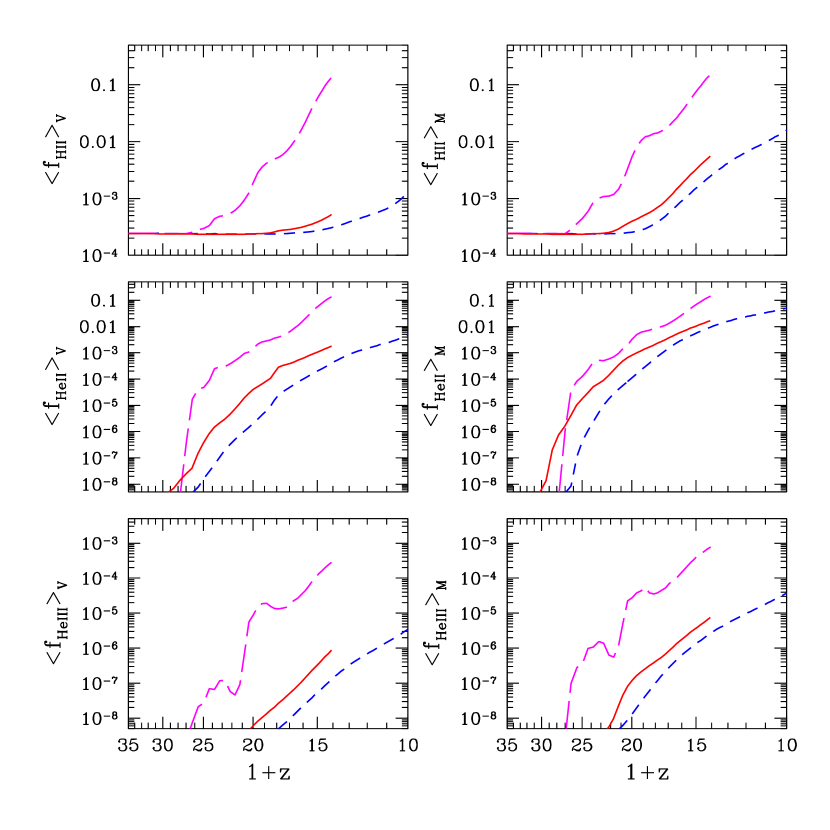
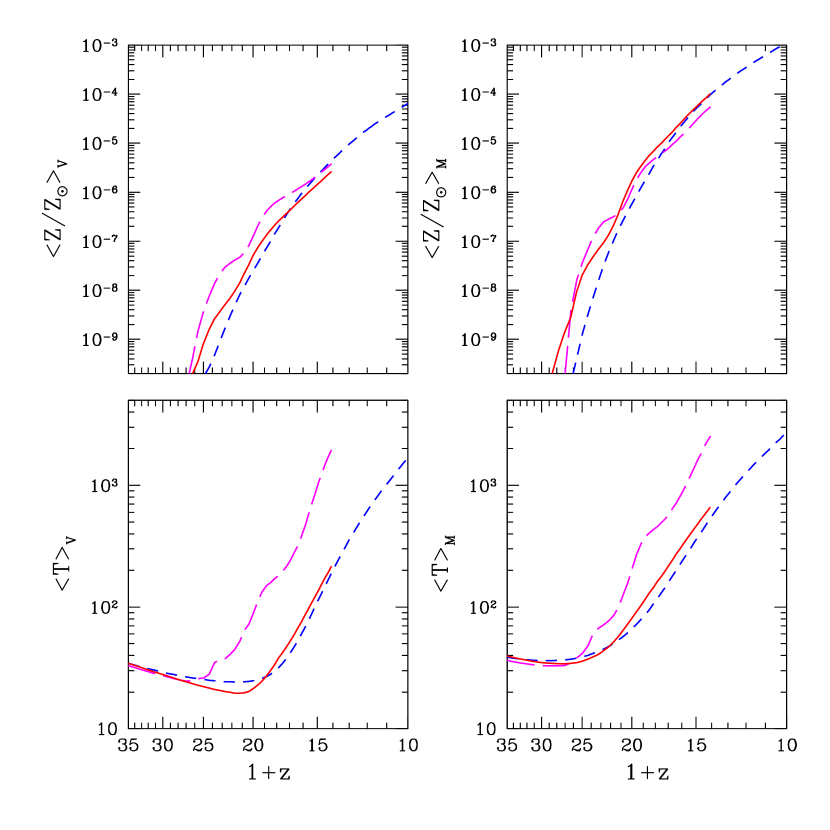
Figure 17: (Top) Mass- and volume-weighted ionized H and He abundances: $\langle x_{{\text{H\,\sc ii}}}\rangle$, $\langle x_{{\text{He\,\sc ii}}}\rangle$, $\langle x_{{\text{He\,\sc iii}}}\rangle$. (Bottom) Mass- and volume-weighted metallicity $\langle Z/Z_{\odot}\rangle$ and temperature $\langle T\rangle$. The solid lines show the 256L1p3 run ($\langle f_{esc}\rangle$ $=0.1$ and $\epsilon_{*}=0.1$), the short-dashed lines the 128L1p2-2 run ($\langle f_{esc}\rangle$ $=0.01$ and $\epsilon_{*}=0.05$), and the long-dashed lines show the 128L1p2 run ($\langle f_{esc}\rangle$ $=1$ and $\epsilon_{*}=0.2$).

The mass-weighted metallicity, $\langle Z/Z_{\odot}\rangle_{M}$, is proportional to the total mass of metals produced by the stars, and therefore is proportional to the SFR. Since we have shown that “small-halo” objects dominate the SFR if $\langle f_{esc}\rangle$ $<1$, at least before redshift $z\sim 10$, their metal production dominates by the same amount. Moreover, we have shown in § 3.3 that, if SF is bursting, photo-evaporation of small galaxies is the main process that pollutes the low-density IGM (voids) with metals. Finally, SNe explosions, not yet included in the simulations, can transport metals into the voids efficiently, since “small-halo” objects are numerous and the voids are small at high redshift.

In Figure 18 (left) we show the evolution of the H i ionizing background $J_{{\text{H\,\sc i}}}$ (thick lines) and the He ii ionizing background $J_{{\text{He\,\sc ii}}}$ (thin lines) for the same three simulations shown in the previous figure. In Figure 18 (right) we show the comoving mean free path of the H i ionizing photons $\lambda_{{\text{H\,\sc i}}}$ (thick lines) and of the He ii ionizing photons $\lambda_{{\text{He\,\sc ii}}}$ (thin lines). Reionization, defined as the overlap of H ii regions, occurs when $\lambda_{{\text{H\,\sc i}}}\sim D_{s}/2\sim 0.1$ $h^{-1}$ Mpc, where $D_{s}$ is the mean comoving distance between the ionizing sources (Gnedin, 2000).

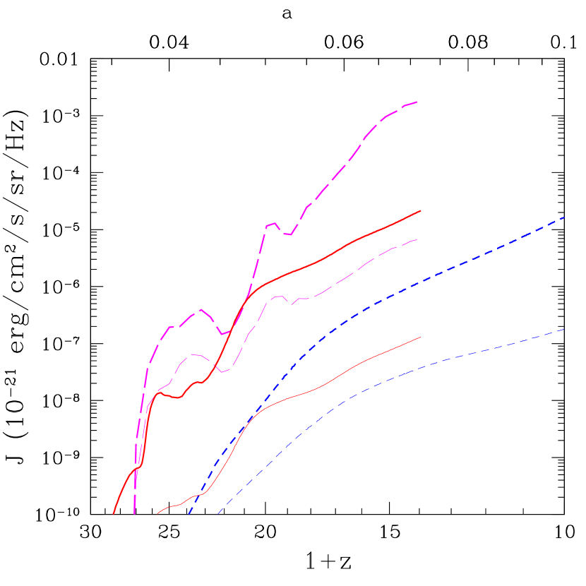
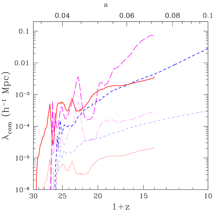
Figure 18: (Left) Evolution of the H i ionizing background $J_{{\text{H\,\sc i}}}$ (thick lines) and the He ii ionizing background $J_{{\text{He\,\sc ii}}}$ (thin lines). (Right) Comoving mean free path of the H i ionizing photons $\lambda_{{\text{H\,\sc i}}}$ (thick lines) and of the He ii ionizing photons $\lambda_{{\text{He\,\sc ii}}}$ (thin lines). The solid lines show the 256L1p3 run ($\langle f_{esc}\rangle$ $=0.1$ and $\epsilon_{*}=0.1$), the short-dashed lines the 128L1p2-2 run ($\langle f_{esc}\rangle$ $=0.01$ and $\epsilon_{*}=0.05$), and the long-dashed lines show the 128L1p2 run ($\langle f_{esc}\rangle$ $=1$ and $\epsilon_{*}=0.2$).

4 Discussion and Summary

In this paper we studied the the formation and evolution of the first galaxies in a $\Lambda CDM$ cosmology. Our results are based on 3D cosmological simulations that include, for the first time, a self-consistent treatment of radiative transfer. The simulations include continuum radiative transfer using the “Optically Thin Variable Eddington Tensor” (OTVET) approximation and line-radiative transfer in the H₂ Lyman-Werner bands of the background radiation. Chemical and thermal processes are treated in detail, particularly the ones relevant for H₂ formation and destruction. The details about the numerical methods and the physics included in the simulations are treated in a companion paper (Paper I). In Paper I we have also performed careful convergence analysis. It appears that we are very close to the convergence limit when we use a $256^{3}$ box. In smaller simulations the SF is underestimated.

The main result is that positive feedback processes dominate negative feedback of the dissociating background, and therefore star formation in “small-halo” objects is not suppressed. The main parameter that determine the importance of “small-halo” objects is $\langle f_{esc}\rangle$. If $\langle f_{esc}\rangle$ $\sim 0.01$, “small-halo” objects dominate the galaxy mass function at least until redshift $z\sim 9$, and feedback produces a bursting SF in these objects. Because the ionization fronts are confined to the dense filaments, reionization of the IGM cannot be produced by “small-halo” objects. However, we find that “small-halo” objects are important in enriching the low-density IGM with heavy elements.

The main processes that are not included in our simulations are H₂ self-shielding and mechanical and thermal energy injection caused by SN explosions. H₂ self-shielding, depending on the choice of the free parameters, could be relevant and should reduce the effects of the dissociating radiation. Since we have found that the dissociating radiation has a negligible role in regulating SF, we expect that the results of our simulations should not be modified by H₂ self-shielding. The effects of dissociating radiation become important when $\langle f_{esc}\rangle$ $\lower 2.15277pt\hbox{$\;\buildrel<\over{\sim}\;$}10^{-3}$. H₂ self-shielding effects probably reduce the value of $\langle f_{esc}\rangle$ for which dissociating radiation becomes important to a smaller value. Although we have not included them in our simulations, SN explosions can be important; their feedback could be responsible for a self-regulating global SF and contribute to spread metals into the low-density IGM. Unfortunately, the dynamical and thermal effects of SN explosions on the ISM of galaxies and IGM are not fully understood. The investigation of the effects of mechanical feedback from SNe explosions will be the subject of our future work.

We cannot rule out alternative cosmologies, in which “small-halo” objects do not form. For example, in warm dark matter (WDM) cosmologies, the free-streaming of the DM particles is large enough to suppress the formation of dwarf galaxies at high redshift. It is also possible that the initial power spectrum does not have enough power on small scales to form “small-halo” objects. Theoretical arguments based on observations of the Ly$\alpha$ forest, quasars at high redshift, and stellar populations in dwarf galaxies pose some constraints on the mass of WDM particle candidates ($m_{wdm}\lower 2.15277pt\hbox{$\;\buildrel>\over{\sim}\;$}1$ keV). Current observations do not rule out these alternative cosmological models; but they may not solve the problems faced by CDM.

In the following list we summarize the results of this work in more detail:

(1) SFR in “small-halo” objects is self regulated and depends only on $\langle f_{esc}\rangle$, for fixed $\epsilon_{UV}$ (known IMF). The SFR is almost independent of the star formation efficiency, $\epsilon_{*}$, the dissociating background, and the SED (metal-free or metal-rich objects) of the sources. It depends only on $\langle f_{esc}\rangle$ and the IMF (number of ionizing photons per baryon converted into stars). If $\langle f_{esc}\rangle$ is small, the SFR is high, while if $\langle f_{esc}\rangle$ $\sim 0.01$ the SF is only slightly suppressed by radiative feedback. In this case, the maximum SFR is proportional to $\epsilon_{*}$, and “small-halo” objects dominate the galaxy mass function at least until redshift $z\sim 10$.

(2) “Small-halo” star formation is intrinsically “bursting”. Star formation is regulated by competing negative and positive feedback from EUV (ionizing) radiation. The H ii regions produced by “small-halo” objects are confined to the dense IGM filaments. Reionization of the IGM cannot happen until massive galaxies are formed. In contrast to massive objects, which reionize voids first, “small-halo” objects partially ionize only the dense filaments while leaving the voids neutral.

(3) Galaxy formation is triggered by the presence of neighboring galaxies. The SFR does not depend strongly on the dissociating background intensity or on the H₂ abundance in the IGM. The self-regulation of star formation relies on H₂ being continuously reformed in positive feedback regions. The H₂ formation happens only in the filaments, both inside relic H ii regions that never expand into the low density IGM and in the H₂ shells just in front of the H ii regions (Ricotti et al., 2001).

(4) The dissociating (FUV) radiation reduces the SFR only if $\langle f_{esc}\rangle$ is very small. If $\langle f_{esc}\rangle$ $\lower 2.15277pt\hbox{$\;\buildrel<\over{\sim}\;$}10^{-3}$ for a Population II SED or $\langle f_{esc}\rangle$ $\lower 2.15277pt\hbox{$\;\buildrel<\over{\sim}\;$}10^{-4}$ for a Population III SED, the negative feedback of the dissociating background suppresses “small-halo” object formation, more efficiently at high-redshift.

(5) “Small-halo” objects dominate the metal pollution of the low-density IGM. The transport of metals from the galaxies to the low-density IGM happens because of the continuous formation and photo-evaporation of small mass (“small-halo”) halos. The metal production, if the SF is self-regulated by EUV radiation, is independent of the SFE, SED, and IMF, but depends only on $\langle f_{esc}\rangle$.

In conclusion, we have shown that, if SN explosions do not suppress the formation of “small-halo” objects and CDM cosmogonies prove to be correct, “small-halo” objects should have profound effects on cosmic evolution. Observations of dwarf spheroidal galaxies, metallicity of the Ly$\alpha$ forest, and stellar populations in the halo of the Milky Way could verify this model. Computational limitations prevent us from evolving a representative sample of the universe to redshifts $z<9$. At lower redshifts, the bulk of “small-halo” objects merge, forming larger mass galaxies, but some of them might survive almost unaffected by the environment. Reionization is probably affecting the ISM of these small galaxies quite substantially, photoevaporating the remaining unshielded gas. These “fossil” “small-halo” objects could be identified with at least some dwarf spheroidal galaxies in the Local Group. In a paper currently in preparation, we study the properties of the simulated “small-halo” objects in order to understand whether this link is real. The prediction of a large population of “small-halo” objects offers a challenging test to verify CDM cosmogonies. We speculate that, in the near future, given the rapid progress of computational power and the rapid growth of observational data of cosmological interest, detailed cosmological simulations will allow us to constrain the evolution of our free-parameters: $\langle f_{esc}\rangle$, $\epsilon_{UV}$, and $\epsilon_{*}$, or possibly the nature of the dark matter.

References

- Becker et al. (2001) Becker, R. H., Fan, X., White, R. L., Strauss, M. A., & Narayanan, V. K. 2001, submitted (astro-ph/0108097)
- Ciardi et al. (2000) Ciardi, B., Ferrara, A., Governato, F., & Jenkins, A. 2000, MNRAS, 314, 611
- Deharveng et al. (2001) Deharveng, J.-M., Buat, V., Le Brun, V., Milliard, B., Kunth, D., Shull, J. M., & Gry, C. 2001, A&A, 375, 805
- Djorgovski et al. (2001) Djorgovski, S. G., Castro, S. M., Stern, D., & Mahabal, A. 2001, submitted (astro-ph/0108069)
- Dove et al. (2000) Dove, J. B., Shull, J. M., & Ferrara, A. 2000, ApJ, 531, 846
- Ferrara (1998) Ferrara, A. 1998, ApJ, 499, L17
- Gnedin (1995) Gnedin, N. Y. 1995, ApJS, 97, 231
- Gnedin (1996) Gnedin, N. Y. 1996, ApJ, 456, 1
- Gnedin (2000) Gnedin, N. Y. 2000, ApJ, 535, 530
- Gnedin & Abel (2001) Gnedin, N. Y., & Abel, T. 2001, New Astronomy, 6, 437
- Gnedin & Bertschinger (1996) Gnedin, N. Y., & Bertschinger, E. 1996, ApJ, 470, 115
- Haiman et al. (2000) Haiman, Z., Abel, T., & Rees, M. J. 2000, ApJ, 534, 11
- Haiman et al. (1997) Haiman, Z., Rees, M. J., & Loeb, A. 1997, ApJ, 476, 458
- Heckman et al. (2001) Heckman, T. M., Sembach, K. R., Meurer, G. R., Leitherer, C., Calzetti, D., & Martin, C. L. 2001, ApJ, 558, 56
- Hurwitz et al. (1997) Hurwitz, M., Jelinsky, P., & Dixon, W. V. D. 1997, ApJ, 481, L31
- Leitherer et al. (1995) Leitherer, C., Ferguson, H. C., Heckman, T. M., & Lowenthal, J. D. 1995, ApJ, 454, L19
- Machacek et al. (2001) Machacek, M. E., Bryan, G. L., & Abel, T. 2001, ApJ, 548, 509
- Ricotti et al. (2001) Ricotti, M., Gnedin, N. Y., & Shull, J. M. 2001, ApJ, 560, 580
- Ricotti et al. (2002) Ricotti, M., Gnedin, N. Y., & Shull, J. M. 2002, ApJ, submitted (Paper I astro-ph/0110431)
- Ricotti & Shull (2000) Ricotti, M., & Shull, J. M. 2000, ApJ, 542, 548
- Steidel et al. (2001) Steidel, C. C., Pettini, M., & Adelberger, K. L. 2001, ApJ, 546, 665
- Wood & Loeb (2000) Wood, K., & Loeb, A. 2000, ApJ, 545, 86