[

Constraining dark energy with Sunyaev-Zel’dovich cluster surveys

Abstract

We discuss the prospects of constraining the properties of a dark energy component, with particular reference to a time varying equation of state, using future cluster surveys selected by their Sunyaev-Zel’dovich effect. We compute the number of clusters expected for a given set of cosmological parameters and propogate the errors expected from a variety of surveys. In the short term they will constrain dark energy in conjunction with future observations of type Ia supernovae, but may in time do so in their own right.

] Recent observations of type Ia supernovae (SNe) have motivated the search for a ubiquitous energy density component, known as dark energy [1]. The defining properties of this energy are that it has negative pressure and does not cluster into galaxies in the same way as dark matter, remaining homogeneous on all but the largest scales. The standard form is the cosmological constant ($\Lambda$), although other possibilities exist including a slowly rolling scalar field [2], known as Quintessence.

The quantification of the properties of this dark energy is now a major part of many observational programs. One proposal is a satellite, known as SNAP (SuperNova Acceleration Probe) [3] which should find around 1800 SNe out to $z\approx 1.7$. This will certainly constrain the properties of dark energy [4, 5], but without prior information on the matter density, $\Omega_{\rm m}$, this will have very little to say about the time evolution of the equation of state parameter $w_{\phi}=p_{\phi}/\rho_{\phi}$, crucial for distinguishing between the various dark energy models [5]. In this Letter, we discuss another approach using future cluster surveys selected using the Sunyaev-Zel’dovich (SZ) effect. We will show that, dependent on the angular coverage ($\Delta\Omega$), frequency ($\nu$) and flux limit ($S_{\rm lim}$), such a survey may provide complementary information to SNe observations, or accurately constrain the properties of the dark energy in its own right.

Observations of clusters via the SZ effect [6] (see ref. [7] for a recent review) exploit the fact that the cosmic microwave background (CMB) radiation is rescattered by hot intracluster gas. Since Compton scattering conserves the overall number of photons, the radiation gains energy by redistributing them from lower to higher frequencies. If one observes them in the Rayleigh-Jeans region of the spectrum, the flux of observed photons decreases compared to the unscattered CMB radiation. The total flux depends on the gas mass and mean temperature of the cluster, but is independent of their distributions. Moreover, the number density of such clusters evolves with redshift under the action of gravity making it an ideal probe of cosmology [8].

The first step is to compute the distribution of clusters which will be observed by a particular survey for a given set of cosmological parameters. We choose to consider the redshift distribution of clusters with mass larger than $M_{\rm lim}\propto\{S_{\rm lim}d_{\rm A}^{2}/[\nu^{2}(1+z)]\}^{3/5}H(z)^{-2/5}$ which is given by

$$\frac{dN}{dz}={\Delta\Omega}\frac{dV}{dzd\Omega}(z)\int\limits_{M_{\rm lim}(z)}^{\infty}\frac{dn}{dM}\,dM\,,$$ (1)

with $\frac{dn}{dM}dM$ the comoving density of clusters with mass between $M$ and $M+dM$, $\frac{dV}{dzd\Omega}$ the volume element, $H(z)$ the Hubble parameter, and $d_{\rm A}$ the angular diameter distance. The distribution $\frac{dN}{dS}$ could also constrain cosmological parameters and may be powerful if there is sparse redshift information available. However, we do not expect it to be very sensitive to the equation of state of dark energy since the crucial redshift dependence is integrated out.

The limiting mass $M_{\rm lim}$ of the survey can be directly related to the total limiting flux $S_{\rm lim}$ of the SZ survey by the virial theorem and the SZ flux [9, 10, 11]. We assume that the geometry of the universe is flat and that the late time dynamics is dominated by a matter component with density $\Omega_{\rm m}$ and a dark energy component with $\Omega_{\phi}=1-\Omega_{\rm m}$. Since there are a wide range of dark energy models discussed in the literature (see refs. [2, 5, 12] and references therein) which all have potentially different late time behaviour we choose to parametrize the equation of state by its late time evolution $w_{\phi}=w_{0}+w_{1}z$. The comoving number density is taken from a series of N-body simulations [13], which yields results similar to using the Press-Schechter formalism  [14], but predicts more massive and less ‘typical’ clusters, as observed in the simulations [15]. The linear growth factor is computed for a given cosmology by solving the ODE for the linear perturbations [9] numerically and non-linear evolution is taken into account via the spherical collapse model.

FIG. 1.: In the left panel we show the cosmology dependence of the redshift evolution of the number of clusters and in the right panel the mass threshold. We vary $\Omega_{\rm m}$, $\sigma_{8}$, $w_{0}$ and $w_{1}$ as explained in the text. The results correspond to the experimental setup (II) with $10^{4}\,{\rm deg}^{2}$ sky coverage.

In Fig. 1 we illustrate the dependence of the redshift distribution of SZ clusters and the limiting mass on cosmology. The solid line is a model with $\Omega_{\rm m}=0.3$, the Hubble constant $H_{0}=65{\rm km}\,{\rm sec}^{-1}{\rm Mpc}^{-1}$, $\sigma_{8}=0.925$, $w_{0}=-1$, $w_{1}=0$ and spectral index of density fluctuations $n=1$. The dotted line has $\Omega_{\rm m}=0.5$, the dashed line $\sigma_{8}=0.975$, the long dashed line $w_{0}=-0.8$ and the dot-dashed line $w_{0}=-0.8$ and $w_{1}=0.3$. The dependence on $n$ is very weak [10] and we therefore fix $n=1$. We will consider the possible dependence of the number density on the parameters $\Theta=(H_{0},\,\sigma_{8},\,\Omega_{\rm m},\,w_{0},\,w_{1})$ in the subsequent analysis. From Fig. 1 we see that $dN/dz$ is strongly dependent on $\Omega_{\rm m}$ and $\sigma_{8}$, while the dependence on $w_{0}$ is still recognizable and that on $w_{1}$ is relatively weak.

We make the optimistic assumption that all the clusters found in the complete surveys can be located sufficiently well so as to determine their redshift out to some critical value $z_{\rm max}$. Furthermore, we will assume that this will be known within a precision of $\Delta z=0.01$ which will allow us to use data bins of size $\Delta z$. This level of accuracy will only require the redshifts to be determined photometrically and will be possible using SDSS (Sloan Digital Sky Survey) and VISTA (Visible and Infrared Survey Telescope for Astronomy). We can then compare to theoretical models using the Cash C statistic [16, 17] for the log-likelihood assuming that the errors are Poisson distributed.

A number of surveys are expected which are designed to detect all clusters above some limiting mass $M_{\rm lim}(z)$. For the purposes of our discussion we will group them into four categories whose observing strategies, approximate $M_{\rm lim}$ and projected number of observed number of clusters in a dark energy based cosmology are tabulated in Table I.

	(I)	(II)	(III)	(IV)
$S_{\rm lim}$	0.1	5	$\approx$36	-
$\nu$	15	30	$\approx$100	-
$\Delta\Omega$	10	$10^{4}$	20600	4000
$M_{\rm lim}$	$1.5$	$\approx 7.0$	$\approx 6.0$	2.5
$N_{\rm tot}$	$\approx 90$	$\approx 1970$	$\approx 5200$	$\approx 13600$
$\delta H_{0}$	$\pm\infty$	$\pm 15$	$\pm 15$	$\scriptstyle{-10/+5}$
$\delta\sigma_{8}$	$\pm 0.075$	$\pm 0.03$	$\pm 0.02$	$\pm 0.007$
$\delta\Omega_{\rm m}$	$\scriptstyle{-0.07/+0.10}$	$\pm 0.05$	$\pm 0.03$	$\pm 0.02$
$\delta w_{0}$	$\scriptstyle{-\infty/+0.30}$	$\scriptstyle{-0.15/+0.29}$	$\scriptstyle{-0.09/+0.12}$	$\scriptstyle{-0.04/+0.12}$
$\delta w_{1}$	$\pm\infty$	$\scriptstyle{-0.60/+0.14}$	$\scriptstyle{-0.46/+0.10}$	$\scriptstyle{-0.55/+0.05}$
$\delta H_{0}$	$\scriptstyle{-15/+5}$	$\pm 5$	$\pm 7$	$\pm 5$
$\delta\Omega_{\rm m}$	$\scriptstyle{-0.04/+0.08}$	$\pm 0.03$	$\pm 0.02$	$\pm 0.01$
$\delta w_{0}$	$\scriptstyle{-0.07/+0.28}$	$\scriptstyle{-0.03/+0.14}$	$\scriptstyle{-0.09/+0.12}$	$\pm 0.03$
$\delta w_{1}$	$\scriptstyle{-\infty/+0.15}$	$\scriptstyle{-0.47/+0.09}$	$\scriptstyle{-0.42/+0.06}$	$\pm 0.03$
$\delta\Omega_{\rm m}$	$\pm 0.04$	$\pm 0.02$	$\pm 0.01$	$\pm 0.01$
$\delta w_{0}$	$\scriptstyle{-0.07/+0.23}$	$\scriptstyle{-0.02/+0.10}$	$\scriptstyle{-0.07/+0.04}$	$\pm 0.03$
$\delta w_{1}$	$\scriptstyle{-\infty/+0.15}$	$\scriptstyle{-0.40/+0.04}$	$\scriptstyle{-0.28/+0.07}$	$\pm 0.03$

TABLE I.: The properties of the different classes of experiments, the number of clusters one would expect to observe in a fiducial cosmology and the 1-$\sigma$ uncertainties on the parameters one would deduce for the same cosmology if one (a) had no prior information, (b) with fixed $\delta\sigma_{8}$ and (c) imposed both $\delta H_{0}=5$ and fixed $\delta\sigma_{8}$ together. The units of ($H_{0}$,$\,S_{\rm lim}$,$\,\nu$,$\,\Delta\Omega$,$\,M_{\rm lim}$) are (${\rm km}\,{\rm sec}^{-1}{\rm Mpc}^{-1}$, mJy, GHz,$\,{\rm deg}^{2}$,$\,10^{14}h^{-1}M_{\odot}$). We used $\infty$ to denote cases where we were unable to make a sensible constraint on a particular parameter.

The first category (I) of deep and narrow surveys contains the interferometric arrays AMI [18] (Arc-minute Micro-Kelvin Imager), SZA  [19] (SZ Array) and AMiBA [20] (Array for Microwave Background Anisotropy). For AMI detailed simulations of the survey yield have been performed and radio source contamination has been considered. The second group (II) are shallow and wide surveys of which OCRA [21] (One-Centimetre Receiver Array) is an example. Here, we use the flux sensitivity for a single receiver from the proposed 100 beam array, without taking into account the effects of atomospheric water vapour at the site. The third class (III), which are shallow but nearly all-sky, correspond to what might be possible based on component separation using the multi-frequency channels of the PLANCK surveyor. As an example of the sensitivity we list the 100 GHz channel. The final category (IV), are deep and wide surveys, such as a 1000 element bolometric array which may be mounted on a telescope at the south pole. In the last case, due to lack of precise figures we will use a constant limiting mass [17].

The 1-$\sigma$ errors one would expect on $\delta\Theta$ are listed in Table I for a fiducial cosmology $\Theta=(65,0.925,0.3,-0.8,0.3)$ assuming no prior information and $z_{\rm max}=1.5$. This particular cosmology was chosen since, firstly, it is in the middle of the parameter range preferred by the current data and, secondly, it corresponds to a particular dark energy model which one might want to constrain [12]. We have tested the stability of our results to small changes in the parameters compatible with the current observational data.

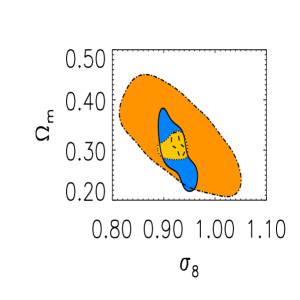
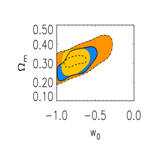
FIG. 2.: The marginalized joint likelihood contours in the $\sigma_{8}$-$\Omega_{\rm m}$ (left) and $w_{0}$-$\Omega_{\rm m}$ (right) planes at the 1-$\sigma$ level. The largest contour corresponds to a type (I) survey, the dark grey contour to type (II), the light grey contour to type (III) and the dashed line contour to type (IV).

The dependence of $dN\over dz$ on $H_{0}$ is very weak and the double-valued nature of growth factor around $w\approx-0.5$ leads to a degeneracy with the amplitude $\sigma_{8}$. Therefore, it seems sensible to consider the possibility of prior assumptions on these two parameters, particularly since both should be measured independently of the properties of the dark energy by other means. $H_{0}$ is measured using the Hubble Space Telescope at present to within $\Delta H_{0}=8$ [22]. We will assume that in the next few years a precise measurement will be possible to $\Delta H_{0}=5$. In the case of $\sigma_{8}$ we will assume that it can be measured almost exactly by, for example, a low-$z$ X-ray survey. Although this will not be precisely true it is useful for comparison with ref. [10]. The results of imposing the prior on $\sigma_{8}$ by itself and combined with that on $H_{0}$ are also listed in Table I.

There is a clear improvement in one’s ability to constrain the parameters in going from a type (I) to type (IV). From the point of view of the dark energy the salient parameters are $\Omega_{\rm m}$, $w_{0}$ and $w_{1}$ whose errorbars are often asymmetric due to the complicated shape of the likelihood surface. Including the prior on $\sigma_{8}$ appears to be useful in removing degeneracies, whereas the distribution is very flat in the $H_{0}$ direction and, therefore, inclusion of a prior on it has little significant effect.

If one uses no prior information with (I), it is only possible to measure $\sigma_{8}$ and $\Omega_{\rm m}$ accurately and place an upper bound on $w_{0}$. There is no viable constraint on $w_{1}$ due to the relatively small number of clusters that one would detect in such a setup. If one includes both the priors $|\delta\Omega_{\rm m}|\approx 0.04$ and a weak constraint on $w_{0}$ is possible, but there is still little information on $w_{1}$.

The results of (II) and (III) are qualitatively similar with (III) improving on (II). With no prior information one can constrain $\sigma_{8}$ and $\Omega_{\rm m}$ considerably ($|\delta\sigma_{8}|$=0.03, $|\delta\Omega_{\rm m}|$=0.05 for (II) and $|\delta\sigma_{8}|$=0.02, $|\delta\Omega_{\rm m}|$=0.03 for (III)), and good information on $w_{0}$ would be possible. However, yet again very little information would be possible on $w_{1}$, a situation which is only mildly alleviated by the inclusion of the prior information. It is worth noting that for our chosen fiducial model it is easier to set an upper bound on $w_{1}$ than a lower bound. This is a general trend we observed for the models we studied, though for some it was less pronounced.

Only in the case of (IV) with a fixed value of $\sigma_{8}$ can very strong statements be made about $w_{1}$ using this kind of observation. Such a setup also gives very accurate information on all the other parameters including $w_{0}$, irrespective any prior. This provides clear motivation for considering the feasibility of this setup.

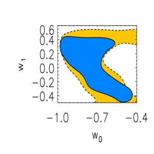
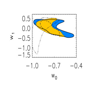
FIG. 3.: The 1-$\sigma$ joint likelihoods in the $w_{0}$-$w_{1}$ plane. In the left panel for setup (II) where dark shaded region is obtained with a maximum redshift of $z_{\rm max}=1.5$ and the light shaded region corresponds to a maximum redshift of $z_{\rm max}=0.5$. In the right panel for setups (II), (III) and (IV) using the same conventions as in Fig. 2. The transparent 3-dot dashed line corresponds to the joint likelihood for the SNe survey SNAP.

We have already noted that the errorbars are in general very asymmetric. In order to investigate this we have plotted in Fig. 2 the joint likelihood surfaces in the $\sigma_{8}$-$\Omega_{\rm m}$ and $w_{0}$-$\Omega_{\rm m}$ planes for each of the setups (I)-(IV), which show visually the relative improvement that one might expect. The degeneracies are similar to those observed in previous work [10] and we see that only (II), (III) and (IV) constrain $w_{0}$ in any significant way. Nonetheless, it is clear that in each case the value of $\Omega_{\rm m}$ is constrained extremely well. We have used $z_{\rm max}=1.5$, however, the using $z_{\rm max}=0.5$ remarkably has little effect on the size of the errorbars, since it is the statistical weight of the large number of clusters found at low redshifts which fixes these parameters. We also performed an analysis with $\Delta z=0.025$ and found that this increases the uncertainties on the estimated parameters in a similar way to changing $z_{\rm max}=1.5$ to $z_{\rm max}=0.5$.

The degeneracy between $w_{0}$ and $w_{1}$ is particularly important from the point of view of dark energy and this is illustrated in Fig. 3, left panel, for (II) under the optimistic assumption that $z_{\rm max}=1.5$ and when $z_{\rm max}=0.5$. The degeneracy has a complicated, double-valued shape and the constrained region is much smaller when $z_{\rm max}$ is larger. This is as expected since constraining these parameters requires more information at high redshifts.

Our results show that only for setup (IV) and an effectively fixed value of $\sigma_{8}$ can one independently fix the crucial parameter $w_{1}$ using this kind of measurement. However, all is not lost; it was pointed out in ref. [5] that given independent prior information on $\Omega_{\rm m}$, SNe measurements can accurately constrain the dark energy. As we have already pointed out even setup (I) will provide important information in this respect and the others will improve on this.

Even more information can be gleaned by making the comparison of the two different probes of dark energy in the $w_{0}$-$w_{1}$ plane. Fig. 3, right panel, illustrates this for setups (II), (III) and (IV) compared to a similar calculation for SNAP [5]. Even for (II) performances of the two methods are comparable in terms of the area of the 1-$\sigma$ contour and for (IV) the result is very much better. Notice also that the degeneracy in this plane is also totally different and combining them would give a localized region pinning down $w_{0}$ very accurately and $w_{1}$ to within $\sim\pm 0.2$. While this may not be enough to rule out $w_{1}=0$ at the 2-$\sigma$ level, a look at the various models for dark energy considered in ref. [5], shows that such observations would put tight constraints on the particular dark energy models.

Our basic philosophy has been to investigate the absolute best case constraints that a given survey can achieve in terms of the properties of the dark energy. In this spirit, we have shown that as with SNe observations, cluster surveys selected using the SZ effect will provide important information as to the nature of the dark energy and that there is a potential synergy between the two. However, our conclusions were drawn from a highly idealized model of cluster physics.

One of the key sources of systematic uncertainties will come from the $M_{\rm lim}-S_{\rm lim}$ relation due to, for example, heat input or the clusters being not completely virialized [23]. These effects might manifest themselves in terms of either a systematic shift in the overall normalization, or in statistical scatter. We have estimated the possible effects of these uncertainties [11] and found that if the scatter is less than about 20% and the overall normalization is accurate to with 5% then one can distinguish our fiducial model from the standard $\Lambda$CDM model. To get an idea of why the constraint on required accuracy of the overall normalization is particularly important we just comment that a 20% change would lead to a factor of 2 change in the total number of clusters.

We are optimistic that many of the practical difficulties which we have ignored will be addressed with the first generation of SZ survey instruments and can be taken into account in the future with the qualitative picture of our results will remain: that SZ cluster surveys provide a robust complementary probe for dark energy.

ACKNOWLEDGMENTS: We thank R. Crittenden, M. Jones and P. Wilkinson for useful discussions. The parallel computations were done at the UK National Cosmology Supercomputer Center funded by PPARC, HEFCE and Silicon Graphics / Cray Research. JW and RB are supported by a PPARC.

REFERENCES

- [1] S. Perlmutter et al., Ap. J. 483, 565 (1997). A. Riess et al., Astron. J. 116, 1009 (1998). S. Perlmutter et al., Ap. J. 517, 565 (1999).
- [2] C. Wetterich, Nucl. Phys. B302, 668 (1988). B. Ratra and P. J. E. Peebles, Phys. Rev. D37, 3406 (1988).
- [3] snap.lbl.gov
- [4] D. Huterer and M. S. Turner, Phys. Rev. D 60, 081301 (1999). I. Maor, R. Brustein and P. J. Steinhardt (2001), Phys. Rev. Lett. 86, 6. Erratum: Phys. Rev. Lett. 87, 049901. P. Astier, Phys. Lett. B 500, 8 (2001).
- [5] J. Weller and A. Albrecht, Phys. Rev. Lett. 86, 1939 (2001). J. Weller and A. Albrecht, astro-ph/0106079.
- [6] R. A. Sunyaev and Ya. Zel’dovich, Comm. Astrophys. Space Phys. 4, 173 (1972). R. A. Sunyaev and Ya. Zel’dovich, MNRAS 190, 143 (1980).
- [7] M. Birkinshaw, Phys. Rep. 310, 97 (1999).
- [8] P. B. Lilje, Ap. J. Lett. 386, L33 (1992). J. Oukbir and A. Blanchard, Astron. and Astro. 262, L210 (1992). V. Eke, S. Cole and C. Frenk, MNRAS 282, 263 (1996). N. A. Bahcall and X. Fan, Ap. J. 504, 1 (1998).
- [9] P. T. P. Viana and A. R. Liddle, MNRAS 281, 323 (1996). L. Wang and P. J. Steinhardt, Ap. J. 508, 483 (1998).
- [10] Z. Haiman et al, Ap. J. 553, 545 (2001).
- [11] J. Weller, R. A. Battye and R. Kneissl, In preparation.
- [12] Ph. Brax and J. Martin, Phys. Lett. B468, 40 (1999).
- [13] A. Jenkins et al., MNRAS 321, 372 (2001).
- [14] W. H. Press and P. Schechter, Ap. J. 187, 425 (1974).
- [15] E. Pierpaoli, D. Scott and M. White, MNRAS 325, 77 (2001).
- [16] W. Cash, Ap. J. 228, 939 (1979).
- [17] G. Holder, Z. Haiman and J. Mohr, Ap. J. Lett. 560, 111 (2001).
- [18] R. Kneissl et al., MNRAS 328, 783 (2001). M. E. Jones, astro-ph/0109351.
- [19] G. P. Holder et al., Ap. J. 544, 629 (2000). J. J. Mohr et al., in ‘Extrasolar Planets to Cosmology: The VLT Opening Symposium’ (2000), edited by A. Renzini, (2000). J. E. Carlstrom et al., in ‘Constructing the Universe with Clusters of Galaxies’ (2000), edited by F. Durret and G. Gerbal, (2000).
- [20] K. Y. Lo et al., in ‘New Cosmological Data and the Values of the Fundamental Parameters’ (2000), edited by A. Lasenby and A. Wilkinson, (2000).
- [21] I. W. Browne et al., in ’Radio Telescopes’ (SPIE Proc. Vol. 4015), edited by H. R. Butcher, (2000).
- [22] W. L. Freedman et al., Ap. J. 553, 47 (2001).
- [23] L. Verde, Z. Haiman and D. N. Spergel, astro-ph/0106315.