The $\alpha$ Dynamo Effects in Laboratory Plasmas

Abstract

A concise review of observations of the $\alpha$ dynamo effect in laboratory plasmas is given. Unlike many astrophysical systems, the laboratory pinch plasmas are driven magnetically. When the system is overdriven, the resultant instabilities cause magnetic and flow fields to fluctuate, and their correlation induces electromotive forces along the mean magnetic field. This $\alpha$-effect drives mean parallel electric current, which, in turn, modifies the initial background mean magnetic structure towards the stable regime. This drive-and-relax cycle, or the so-called self-organization process, happens in magnetized plasmas in a time scale much shorter than resistive diffusion time, thus it is a fast and unquenched dynamo process. The observed $\alpha$-effect redistributes magnetic helicity (a measure of twistedness and knottedness of magnetic field lines) but conserves its total value. It can be shown that fast and unquenched dynamos are natural consequences of a driven system where fluctuations are statistically either not stationary in time or not homogeneous in space, or both. Implications to astrophysical phenomena will be discussed.

1. Introduction

Phenomena involving magnetic field have been observed in astrophysical systems ranging from planets and stars to accretion disks, galaxies and even in clusters of galaxies [1]. Understanding the origins and effects of these cosmic magnetic fields has been one of most active research areas across multiple subdisplines of physics. In particular, generation and sustainment of magnetic fields from dynamics in electrically conducting media, or so-called dynamo actions [2], has long remained an unsolved problem.

A typical astrophysical system is driven by a combination of thermal, rotational, and gravitational energies. For example, dynamics in the outer core of the earth is dominated by Coriolis force (due to rotation) and thermal convection (due to temperature gradient and gravity). Another example is the accretion disks where the differential rotation is a primary source of free energy originating from the release of gravitational energy. Magnetic field in these systems can grow out of corresponding instabilities. Often, the resultant Lorentz force is ignored in the equation of the motion, i.e., the so-called kinematic dynamo problem. When the Lorentz force is fully taken into account in the flow dynamics, the problem is nonlinear.

In the kinematic dynamo problem, the flow velocity is completely determined by the corresponding free energy source, either thermal, rotational, or gravitational. The growth of magnetic field is only passively determined as a linear problem, and is not a part of dynamics. The kinematic dynamo introduces simplicity, but does not provide a self-consistent solution for either the flow or magnetic field.

The dynamos in astrophysical systems are mostly fully nonlinear in nature. The effects of magnetic field must be fully taken into account i.e., the Lorentz force is an integral part of the dynamics, often resulting in saturation of the magnetic field growth. In most cases, however, the nonlinear dynamos are too complicated to be studied theoretically without invoking statistical treatments. One such example is the so-called mean-field electrodynamics [3], where the ensemble-averaged electromotive force is calculated along the mean magnetic field (the $\alpha$-effect) or the mean electric current (the $\beta$-effect).

The mean electromotive force generates and sustains the entire mean magnetic field or current, which, in turn, influences the dynamo effects. This is true in all the astrophysical systems driven non-magnetically. When a system is driven magnetically, i.e. the free energy source is in the magnetic form, the electromotive force or the $\alpha$-effects still modify the externally supplied mean magnetic field. Sometimes the modifications are so significant that the resultant mean field is qualitatively different from its initial profile. This article is intended to describe such an example in laboratory pinch plasmas which are driven only magnetically. The observed $\alpha$-effects exhibit remarkably similar properties to those in astrophysical systems: they modify the mean magnetic profile in a time-scale much faster than resistive time scale, and they are closely related to the concept of magnetic helicity as shall be described later. The laboratory elucidates key aspects of dynamo physics since detailed measurements are possible, and the MHD nonlinear problem can be formulated and solved.

The remainder of this paper is organized as follows: qualitative introduction to laboratory pinch plasmas is given in Sec. 2, including demonstration of the need for a dynamo mechanism to explain magnetic field generation. The nonlinear MHD description of the dynamo is summarized in Sec. 3, including the role of the dynamo in the self-organization of the plasma, and the instabilities that underlie the process. Experimental measurements of $\alpha$-dynamo effects are presented in detail in Sec. 4. The nature of the observed dynamo effects and their relation to magnetic helicity are discussed in Sec. 5, followed by implications to the astrophysical dynamos and conclusions in Sec. 6.

2. Pinch plasmas: magnetically driven systems

Figure 1: Coordinates for toroidal geometry: the cylindrical coordinate (major radius $R$, toroidal angle $\phi$, axial direction $Z$) and the toroidal coordinate (toroidal angle $\phi$, poloidal angle $\theta$, and radius $r$). The aspect ratio of a torus is defined as $R_{0}/a$.

The history of pinch plasma experiments goes back to early 1950’s as a part of efforts for development of magnetically confined plasmas for the nuclear fusion application. The basis of these experiments is the pinch effect, in which a current channel in the electrically conducting plasmas contracts through the self-magnetic field of the current. The current can be driven either by a voltage applied between electrodes or electromagnetic induction through a transformer. We shall focus on a subclass of the pinch experiments that are toroidal (Fig. 1), where most of relevant theoretical and experimental dynamo work have been performed. Specifically, the reversed-field pinch (RFP) plasmas [4, 5] shall be described in detail. A similar configuration known as spheromak [6, 7] shall also be mentioned but the interested readers should refer to the review papers mentioned above for some experimental details.

2.1. Formation of pinch plasmas

The RFP plasmas are produced by an inductive electric field along the toroidal direction through a transformer. The plasma serves as the secondary coil of the transformer. A typical experimental arrangement is conceptually illustrated in Fig. 2, where the plasma is surrounded by a metal shell. The electrical skin time of the shell is much longer than the experimental time thus it can be considered as an ideal conductor to ensure that the magnetic field lines are always parallel to the shell surface. The shell has gaps along toroidal and poloidal directions permitting instantaneous penetration of the applied electric field.

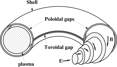
Figure 2: Illustration of an RFP plasma with its magnetic field at several radii. The toroidal component reverses its direction at the edge.

The time evolution of magnetic field and current density profiles as functions of $r$ are qualitatively shown in Fig. 3. Initially ($t\leq t_{0}$), a uniform toroidal magnetic field is imposed [Fig. 3(a)]. At $t=t_{0}$, the toroidal electric field is applied through the transformer to drive the toroidal current, which, in turn, produces the poloidal magnetic field. Therefore, the field lines become helical. Since the electrons freely move along the field lines but not so across the field lines, the current path also becomes helical with a poloidal component. The poloidal current modifies the initially imposed toroidal field. Figure 3(b) illustrates the magnetic and current profiles at a time $t=t_{1}>t_{0}$, when the modification to the initial field is relative small. (This corresponds to the tokamak configurations, another subclass of toroidal pinch plasmas.) We note that the toroidal field increases at the center but decreases at the edge.

Figure 3: Qualitative illustration of time evolution of the normalized magnetic field and current density profiles in a pinch plasma when the electric field is increased in sequence: (a) initial state where only toroidal field exists; (b) small electric field to drive mainly toroidal current in tokamaks; (c) modest electric field to significantly drive both toroidal and poloidal current components; (d) and finally an RFP configuration is realized when the toroidal magnetic field reverses its direction.

If the applied toroidal electric field is raised further raised, the amplitude of both toroidal and poloidal currents increases to further modify the field profiles. The poloidal field approaches to the magnitude of the toroidal field, while the toroidal field continues to peak at the center and diminish at the edge, as illustrated in Fig. 3(c) for $t=t_{2}>t_{1}$. Finally, when the electric field is raised to a large enough value, the toroidal field eventually reverses its direction at the edge [Fig. 3(d) for $t=t_{3}>t_{2}$,] the origin of the name of reversed-field pinch (RFP). Figure 2 also illustrates magnetic structures at various radii. Since the center toroidal field increases by a much larger value than the edge value decreases, the total toroidal flux is amplified significantly.

The spheromak plasma configuration is similar to the RFP. It contains helical field lines, with the field at the edge being mainly poloidal. The spheromak is a torus with aspect ratio of unity (no hole in the center). An additional difference from the RFP is that the electric field that drives the initial current is mainly poloidal and localized at the plasma edge. Nonetheless, the observed dynamo effects are strikingly similar to those in the RFP. Therefore, the rest of this paper shall focus on RFP plasmas.

Figure 4: Mismatch between the applied electric field $E_{\parallel}$ and the resistive counterpart $\eta j_{\parallel}$ along the field line at $t=t_{4}$ of Fig. 3(d). It is noted that $E_{\parallel}>\eta j_{\parallel}$ at the center (often called anti-dynamo) while $E_{\parallel}<\eta j_{\parallel}$ at the edge (dynamo).

2.2. Need for a dynamo effect

The current density and magnetic field profile in the RFP, particularly the reversal of the toroidal magnetic field, cannot arise in a steady-state plasma that is toroidally symmetric (lacking in symmetry-breaking fluctuations). This can be seen easily by comparing terms in the MHD Ohm’s law parallel to the magnetic field,

$$E_{\parallel}=\eta j_{\parallel}.$$ (1)

The parallel component of electric field, $E_{\parallel}$, can be calculated by ${\bf E\cdot B}/B=E_{\phi}B_{\phi}/B$, where $E_{\phi}$ is the fully penetrated electric field and $B=\sqrt{B_{\phi}^{2}+B_{\theta}^{2}}$. Since both $E_{\phi}$ and $B$ are a constant, $E_{\parallel}$ has the shape of $B_{\phi}$ which reverses its sign at the edge. On the other hand, $\eta j_{\parallel}$ never changes its sign across the radius, as shown in Fig. 4. As a result, the edge parallel current, essentially in the poloidal direction, flows against an externally applied electric field. Thus, the parallel component of Ohm’s law cannot be satisfied without additional terms, such as the $\alpha$-effect.

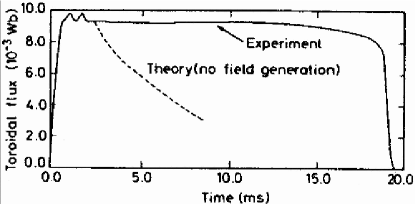
Figure 5: Time evolution of toroidal flux: measurement and calculation with no dynamo effects in an RFP plasma[8]. Note that the decay around $t=18$ms is due to termination of the applied electric field.

The need for a dynamo effect can also be inferred by comparing the measured toroidal flux with that predicted from a simple, symmetric resistive MHD theory. Figure 5 shows an example of the measured time evolution of toroidal flux together with that calculated by resistive MHD theory without dynamo effects. Interestingly, the toroidal flux is sustained as long as the toroidal electric field is provided in the experiment, while the flux decays away in the theory. Clearly, existence of dynamo effects is required to explain both amplification and sustainment of the toroidal flux.

3. Self-Organization and the MHD Dynamo

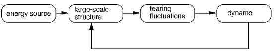
Figure 6: Schematic of magnetic self-organization in laboratory plasmas.

The dynamo effect in laboratory plasmas is part of a self-organization process. Resistive diffusion evolves the plasma away from a preferred state; the dynamo forces the plasma back toward the preferred, self-organized state. The macroscopic features of magnetic self-organization are described in Sec. 3.1. Resistive diffusion is well-understood; the large scale-self-organization driven by the dynamo is a current topic of research and the focus of this paper. Single-fluid MHD equations provide a fully nonlinear description of the dynamo in laboratory plasmas. The fluctuations, in velocity and magnetic field, and the large-scale mean magnetic field, are all determined self-consistently. The MHD calculations include both the effect of the fluctuations on the mean field and the effect of the mean field on the fluctuations. Weakly nonlinear analytic calculations capture some of the key physics, and computational solution of the nonlinear, three-dimensional resistive MHD equations provide a complete description. The fluctuations that underlie the dynamo arise from tearing instabilities. A brief discussion of tearing instabilities in the laboratory context is included in Sec. 3.2. A description of some of the key results of the nonlinear problem is presented in Sec. 3.3.

3.1. Magnetic self-organization

The dynamo effect underlies magnetic self-organization in the laboratory [9]. The plasma is driven by an applied electric field as seen in Sec. 2.1. The resulting magnetic configuration has excess free energy leading to instabilities (or turbulence) that relax the plasma toward a state of lower magnetic energy. The plasma relaxes to the lower energy state through the dynamo effect. The self-generation of plasma current reconfigures the large-scale magnetic field to one with lower energy. This process is depicted in Fig. 6.

The structure of the relaxed state is partly captured by minimizing the magnetic energy in the plasma volume ($W=\int(B^{2}/2\mu_{0})dV$) subject to the constraint of constant magnetic helicity ($K=\int{\bf A}\cdot{\bf B}dV$), where ${\bf A}$ is the magnetic vector potential). Magnetic helicity is a topological measure of the knottedness of the magnetic field lines [10]. The minimization yields a magnetic field given by $\nabla\times{\bf B}=\mu{\bf B}$, where $\mu$ is a constant. Thus, the ratio of the current density to magnetic field, $j/B$, is a spatial constant. This relaxed state is sometimes referred to as the Taylor state. For a one-dimensional cylindrical plasma (where ${\bf B}={\bf B}(r)$) the solution yields Bessel functions, $B_{z}=B_{0}J_{0}(\mu r)$, $B_{\theta}=B_{0}J_{1}(\mu r)$, where $B_{0}$ is a constant. The noteworthy feature of this solution, shown in Fig. 7, is that it approximates the measured profiles of the reversed field pinch shown in Fig. 3d (identifying $B_{z}$ with the toroidal field and $B_{\theta}$ with the poloidal field). In particular, the reversal of the toroidal field is obtained.

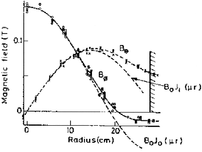
Figure 7: Solution for axial and azimuthal magnetic field of the relaxed state and its comparisons with the measurements [5].

The driven/relaxation phenomenon can occur in experiment in either a continuous or cyclic fashion. The drive forces the plasma away from the relaxed state, and the dynamo opposes this tendency. In some experimental plasmas, the net result is that these effects are nearly balanced at all times; thus, the plasma mean field is approximately steady in time. In other experimental plasmas, the two effects are separated in time citeWatt83,Hokin91. During the drive period, the plasma slowly evolves away from the relaxed state, driven by the applied electric field. During the relaxation period, the dynamo rapidly returns to the plasma to a relaxed. This sawtooth cycle is evident experimentally in the toroidal magnetic flux in the plasma, shown in Fig. 8. A slow decay of the flux is followed by rapid magnetic flux generation by the dynamo. The dynamo acts as discrete events in time. During the decay phase the ratio $j/B$ is becoming spatially peaked; during the relaxation phase it becomes flatter. Relaxation processes happen also in spheromak plasmas [13] where the driving electric field can be either in toroidal or poloidal direction with the aspect ratio, $R_{0}/a$, close to unity, but the underlying physics of relaxation is essentially the same.

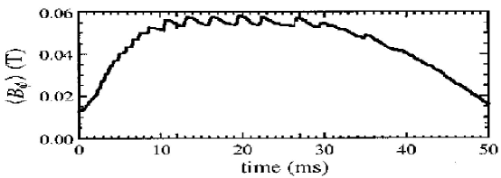
Figure 8: Toroidal magnetic flux versus time in an RFP experiment.

An experimental test of the Taylor conjecture was achieved by inferring the change in magnetic energy and helicity during a relaxation event [14]. An approximate measurement was obtained by modeling the instantaneous plasma state as a slowly varying MHD equilibrium. Since the fields during relaxation are changing on a time scale longer than an Alfven time, the fields will satisfy the MHD force balance equation, ${\bf j}\times{\bf B}=\nabla p$, through a discrete dynamo event. Through solution of this equation with experimental constraints it is found that during a relaxation event the magnetic energy reduces by about 8%, while the magnetic helicity reduces by about 3%, as shown in Fig. 9. (Also see Sec. 5.4)

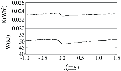
Figure 9: Time evolution of total magnetic helicity and energy during relaxation event in an RFP plasma [14].

3.2. Magnetic (tearing) instabilities

The Taylor conjecture provides a useful framework to depict approximately the final state of the relaxation, or dynamo, process. However, it provides no information on the physical mechanism of the dynamo. Solution of the resistive nonlinear MHD equations reveals the detailed dynamics. The spatial fluctuations that underlie the dynamo are tearing instabilities. Tearing instabilities are driven by spatial gradients in $j/B$, and cause the field lines to tear and reconnect [15]. The MHD description of such spontaneous magnetic reconnection has been investigated for several decades. From linear theory, it is known that tearing instabilities grow on a timescale that is intermediate between short Alfven time ($a/V_{A}$, where $V_{A}=(B^{2}/\mu_{0}\rho)^{1/2}$ and $\rho$ is the mass density) and the long resistive diffusion time ($\mu_{0}a^{2}/\eta$, where $\eta$ is the resistivity). For the experimental plasma parameters, the theoretical growth time is approximately 100$\mu s$, comparable the observed fast relaxation time.

The tearing instability can be described by a wave function of the form $f(r)\exp[i(m\theta-n\phi)]$ where m and n are integers representing the poloidal and toroidal mode numbers. In laboratory plasmas, many tearing modes can be present simultaneously. For tearing to occur, the fluctuating field must be constant along the mean magnetic field. That is, the parallel wave number must vanish (parallel wavelength must become infinite) somewhere in the plasma. This condition ($k_{\parallel}=0$) becomes

$${\bf k}\cdot{\bf B}=k_{\theta}B_{\theta}+k_{\phi}B_{\phi}={m\over r}B_{\theta}-{n\over R}B_{\phi}=0.$$ (2)

The condition can be written as $q=m/n$ where $q=rB_{\phi}/RB_{\theta}$ is the winding number of the mean magnetic field and varies with minor radius. This condition represents a resonance between the fluctuating and mean magnetic fields. In laboratory plasma discussed here, multiple tearing modes with multiple mode numbers occur. Hence, tearing occurs at many radii within the plasma, leading to large-scale reorganization.

3.3. The nonlinear MHD dynamo

An $\alpha$-effect dynamo arises from MHD tearing instabilities, as indicated in the mean-field Ohm s law

$$\overline{\bf E}+\langle\widetilde{\bf v}\times\widetilde{\bf B}\rangle=\eta\overline{\bf j}$$ (3)

where the tilde denotes fluctuations and $\langle~{}\rangle$ denotes mean quantities (averages over the poloidal and toroidal directions). Some key features of the dynamo electromotive force that arises from the fluctuations can be discerned from quasilinear theory. In quasilinear theory the alpha effect term (the second term on the left hand side) is evaluated from the solutions for the fluctuations obtained from linear stability theory. In linear theory the mean field is specified; the spatial structure and the growth rate of the exponentially growing modes are calculated. From quasilinear theory the parallel component of the alpha effect in the vicinity of the radius about which reconnection occurs is found to be [16, 17]

$$\langle\widetilde{\bf v}\times\widetilde{\bf B}\rangle_{\parallel}=\nabla\cdot\left(D\nabla{\overline{j}\over B}\right)$$ (4)

This indicates that the dynamo effect drives current so as to reduce the gradient in $j/B$, consistent with a relaxation in the direction of the Taylor state. The dynamo is in the form of a diffusion mechanism. The diffusion coefficient is proportional to $\widetilde{B}^{2}$.

Quasilinear theory is incomplete. It only captures the dynamo effect during the growing phase of the instability. Extensive computational study has produced a fully self-consistent description of the MHD laboratory dynamo. The nonlinear computation predicts a steady state dynamo, and includes the interaction between the fluctuations and mean fields (the quasilinear effect) and the nonlinear energy transfer between different spatial Fourier modes. Computation predicts that the fluctuation energy is spread over a modest number of nonlinearly interacting modes, of order of the aspect ratio, $R_{0}/a$. From an initial state of random noise, the instabilities grow (excited by the gradient in $j/B$), reaching an amplitude of about 1% of the mean field. The radial profile of each of the terms in the parallel (to $\overline{\bf B}$) component of the mean-field Ohm’s law is displayed in Fig. 10. Note that the alpha effect is large. At the radius where the mean parallel electric field is zero, all the current is driven by the dynamo. Since the alpha effect reverses sign with radius, it can also be viewed as redistributing current from the center the edge.

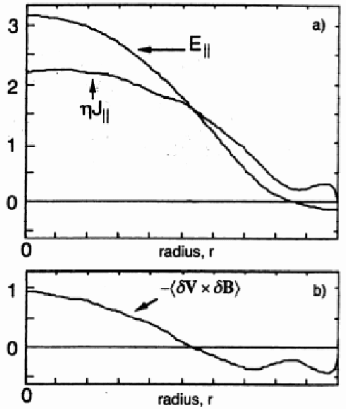
Figure 10: Radial profile of each term in the mean-field Ohm’s law, showing (a) the mean electric field and current density and (b) the fluctuation-induced dynamo term. Each term is evaluated from nonlinear MHD computation.

4. Measurements of Dynamo Effects

Despite the long history of research of RFP plasmas and subsequent recognition of existence of dynamo effects, the experimental efforts to directly measure the $\alpha$-effect did not start until the late 1980’s [18]. The main reason is the difficulty in measuring local velocity fluctuations of both ions and electrons in a plasma. Below we describe several techniques successfully used to measure the velocity fluctuations, thus the dynamo effects. In addition to the MHD dynamo, discussed in the previous section, measurement have been made to examine dynamo effects arising from pressure effects, the Hall term, and kinetic effects. We discuss each of these four dynamo mechanisms in turn.

4.1. MHD dynamo

The key quantity to measure is the component of the fluctuation-induced electromotive force along the mean magnetic field. In the MHD model, where ${\bf v}$ is dominated by the ${\bf E}\times{\bf B}$ drift, the electron and ion velocities are about equal. The corresponding term is $\langle\widetilde{\bf v}\times\widetilde{\bf B}\rangle_{\parallel}\simeq\langle\widetilde{\bf v}_{\perp}\times\widetilde{\bf B}_{\perp}\rangle_{\parallel}$. Thus, the key is to measure $\widetilde{\bf v}_{\perp}$ with sufficient time and spatial resolutions.

The first technique invokes measurements of fluctuations in the perpendicular electric field. The measuring principle is based on the fluctuating Ohm’s law, $\widetilde{\bf E}+\widetilde{\bf v}\times\overline{\bf B}+\overline{\bf v}\times\widetilde{\bf B}=\eta\widetilde{\bf j}$, which reduces to

$$\widetilde{\bf v}_{\perp}={(\widetilde{\bf E}_{\perp}+\overline{\bf v}\times\widetilde{\bf B}-\eta\widetilde{\bf j}_{\perp})\times\overline{\bf B}\over\overline{B}^{2}}\simeq{\widetilde{\bf E}_{\perp}\times\overline{\bf B}\over\overline{B}^{2}},$$ (5)

because $\widetilde{\bf E}_{\perp}\gg\eta\widetilde{\bf j}_{\perp}$ and $\widetilde{\bf E}_{\perp}\gg\overline{\bf v}\times\widetilde{\bf B}$ in typical conditions. Therefore, the $\alpha$-effect becomes

$$\langle\widetilde{\bf v}\times\widetilde{\bf B}\rangle_{\parallel}\simeq{\langle(\widetilde{\bf E}_{\perp}\times\overline{\bf B})\times\widetilde{\bf B}_{\perp}\rangle\over\overline{B}^{2}}={\langle\widetilde{\bf E}_{\perp}\cdot\widetilde{\bf B}_{\perp}\rangle\over\overline{B}}.$$ (6)

Fluctuations in electric and magnetic fields and their correlations can be measured by Langmuir probes and magnetic pickup coils, respectively, at the plasma edge where the temperature is relatively low [19]. However, the first attempt using this technique in a relatively dense RFP plasma measured [18] no perceivable $\alpha$-effect compared to the mismatch between $E_{\parallel}$ and $\eta j_{\parallel}$ shown in Fig. 4. It has been suggested later that another mechanism (see next subsection) for the dynamo action might be operational in these dense plasmas.

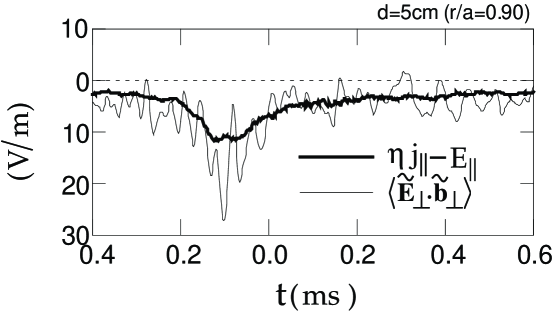
Figure 11: Time evolution of the measured MHD dynamo electric field $\langle\widetilde{\bf E}_{\perp}\cdot\widetilde{\bf B}_{\perp}\rangle/\overline{B}$ by Langmuir probes [20] in MST, compared with the mismatch $\eta j_{\parallel}-E_{\parallel}$ in the parallel Ohm’s law during a relaxation cycle.

The first successful detection [20] of the MHD dynamo in the RFP plasmas was made in the well-controlled Madison Symmetric Torus (MST) plasmas. As discussed in Sec. 3.1, in addition to the continuous dynamo action to regenerate toroidal flux against resistive diffusion, discrete relaxation events occur in MST in a regular fashion to generate toroidal flux in a short time scale. Figure 11 displays the measured dynamo electric field compared with the mismatch between $E_{\parallel}$ and $\eta j_{\parallel}$. The agreement is excellent both during relaxation events ($t\simeq-0.1$ms) and between events. Successful measurements of MHD dynamo effects were made in a spheromak using a similar technique [21].

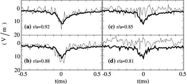
Figure 12: Time evolution of the measured MHD dynamo electric field $\langle\widetilde{\bf v}\times\widetilde{\bf B}\rangle_{\parallel}$ (light line) by an optical probe [23] in MST, compared with the mismatch $\eta j_{\parallel}-E_{\parallel}$ (heavy line) in the parallel Ohm’s law during a relaxation cycle.

The second technique used to measure fluctuating velocities is spectroscopic detection of the Doppler shift from impurity carbon ions embedded within the hydrogen plasmas [22, 23]. If the coupling between impurity ions and plasma ions are strong, or they behave in the same way when exposed to the slow electric field fluctuations, the emission from impurity ions function as a tracer of plasma flow. An optical probe [24] was utilized to measure local velocity fluctuations of impurity ions. Correlations with local magnetic fluctuations have also yielded remarkable agreement with the mismatch electric field at the edge as shown in Fig. 12. At smaller radii, however, the measured dynamo term diminishes due to the phase changes in $\widetilde{v}_{r}$ [23]. Other mechanisms discussed in Sec. 3 for the dynamo effects might be operational at the smaller radii.

4.2. Diamagnetic dynamo

Because of the collisionless nature of high temperature plasmas, MHD approximations are not always a good model to describe dynamics of such plasmas. A better model can be based on the two-fluid model where ion fluid and electron fluid are treated separately. As described in Sec. 3.3, the force balance for electrons is essentially the Ohm’s law, which is generalized to include electron pressure force,

$${\bf E}+{\bf v}_{e}\times{\bf B}+{\nabla P_{e}\over en}=\eta{\bf j},$$ (7)

where the electron inertial effect is ignored. Then Eq.(6) is modified to

$$\langle\widetilde{\bf v}_{e}\times\widetilde{\bf B}\rangle_{\parallel}\simeq{\langle\widetilde{\bf E}_{\perp}\cdot\widetilde{\bf B}_{\perp}\rangle\over\overline{B}}+{\langle{\bf\nabla}_{\perp}\widetilde{P}_{e}\cdot\widetilde{\bf B}_{\perp}\rangle\over e\overline{n}\overline{B}}$$ (8)

where the second term is referred as “diamagnetic” dynamo since the fluctuating electron velocity is due to electron diamagnetism. We note that a small “battery” term is ignored here (see Sec. 5.1.)

The diamagnetic dynamo has been detected at the edge of an RFP plasma when the density is high [25]. Fluctuations in the electron pressure (density and electron temperature) can be measured by Langmuir probes at different locations to deduce their gradient. Figure 13 shows the cross spectra of fluctuating quantities for both MHD dynamo and diamagnetic dynamo for four different densities. In the low density plasmas, the MHD dynamo dominates while at the highest density, the diamagnetic dynamo dominates. Although the underlying mechanisms for the transition are still unclear, this observation is consistent [26] with the early measurements in a dense plasma where no significant MHD dynamo was detected [18].

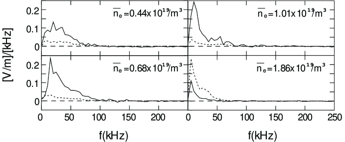
Figure 13: Cross spectra of the MHD (solid lines) and diamagnetic dynamo (dotted lines) terms for four different density cases in a RFP plasma [25].

4.3. Hall dynamo

Since ${\bf j}=en({\bf v}_{i}-{\bf v}_{e})$ and ${\bf v}\approx{\bf v}_{i}$, Eq.(7) can be written as

$${\bf E}+{\bf v}\times{\bf B}-{{\bf j}\times{\bf B}\over en}+{\nabla P_{e}\over en}=\eta{\bf j},$$ (9)

where the second term in the left-hand side is called the Hall term. The fluctuation-induced counterpart, $\langle\widetilde{\bf j}\times\widetilde{\bf B}\rangle/en$, therefore called Hall dynamo, has been suggested to be important under certain conditions [27]. Experimentally, current density fluctuations can be measured by magnetic pickup coils, placed at several spatial points, using Ampere’s law. Measurements at the plasma edge indicated small but non-negligible effects in the Ohm’s law [28].

Physically, the Hall dynamo arises when electron flow does not fluctuate together with ions in the perpendicular direction. For this to happen, electrons need to experience different forces than ions. Electric force cannot be the cause since its fluctuations induce only the same flow fluctuations for both species. However, the electron pressure force can serve this purpose by driving flows only in electrons. Therefore, the diamagnetic dynamo mentioned above is a manifestation of the Hall dynamo effect. Another possibility for a finite difference in perpendicular flows of electrons and ions has been suggested [25, 27] when the viscous force for ions is large.

4.4. Kinetic dynamo

For ions and electrons to be treated as fluids, their distribution functions need to be close to Maxwellians. In the collisionless plasmas, however, this cannot be always true especially in the pinch plasmas driven by a large electric field. In such cases, often a high-energy tail of electrons form along magnetic field line. When the field lines wander from center to edge, these high-energy electrons follow, resulting in transport of electric current outward. The current transport due to these electrons can just make up the mismatch in the electric field illustrated in Fig. 4. The physics process, however, needs to be treated by the full kinetic equations, referred as the kinetic dynamo theory [29]. The main support for this theory is from the observation [30] of high energy electrons along the field lines carrying most of the current, as exemplified in Fig. 14.

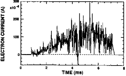
Figure 14: Time evolution of energetic electron current measured by an electrostatic electron energy analyzer with the entrance aligned along the field line at the edge of an RFP plasma [30].

However, the present form of this theory does not include the effects of these energetic electrons on the dynamics of magnetic field lines through Ampere’s law. It has been pointed out [31] that such dynamical feedback to the magnetic field structure would impose a severe constraint on the efficiency of this mechanism. Alternately, the observation of energetic electrons is possibly just a manifestation of other dynamo processes motioned above, i.e., they are accelerated by local dynamo electric field [32]. Kinetic behaviors of the plasma in such a turbulent environment may be far from a simple physics picture.

5. Implications to Dynamo Theories and Astrophysical Dynamos

What we can learn from the observed dynamo effects described in the previous sections? In this section, we discuss their implications to a number of important and often controversial issues in recent developments in dynamo theory: fast dynamo versus slow dynamo; back-reaction of mean field on dynamo action; stationary and homogeneous turbulence versus driven systems; and its relationship with magnetic helicity. Finally, implications to astrophysical systems, especially the solar dynamo problem, are discussed.

5.1. Fast dynamo versus slow dynamo

Fast dynamos are dynamo actions which do not diminish in the small resistivity limit, while slow dynamos do. Fast dynamos can change the magnetic field in a much faster time scale than the resistive diffusion time, in which slow dynamos operate. A real solution for the astrophysically observed dynamos must be a fast dynamo. In fact, the dynamo effects described in the previous section are evidently also fast dynamos, which can change the magnetic flux in a time scale (typically $\sim 100\mu$s during relaxation events) much faster than the resistive diffusion time (typically $\sim 0.1$s).

For clarity, we re-derive the $\alpha$-effect based on the Ohm’s law in the two-fluid framework, Eq. (7), ${\bf E}+{\bf v}_{e}\times{\bf B}+\nabla P_{e}/en=\eta{\bf j}$. After ensemble-averaging over fluctuations it becomes

$$\overline{\bf E}+\overline{\bf v}_{e}\times\overline{\bf B}+\langle\widetilde{\bf v}_{e}\times\widetilde{\bf B}\rangle+{\nabla\overline{P}_{e}\over en}=\eta\overline{\bf j},$$ (10)

which can be subtracted from Eq. (7) to yield

$$\widetilde{\bf E}+\widetilde{\bf v}_{e}\times\overline{\bf B}+(\overline{\bf v}_{e}+\widetilde{\bf v}_{e})\times\widetilde{\bf B}-\langle\widetilde{\bf v}_{e}\times\widetilde{\bf B}\rangle+{\nabla\widetilde{P}_{e}\over en}=\eta\widetilde{\bf j},$$ (11)

where small battery-like effects such as $\langle\widetilde{n}\nabla\widetilde{P}_{e}\rangle/e\overline{n}^{2}$ are neglected (see Sec. 5.4). With the use of Eq. (11), the $\alpha$-effect is calculated as

$$\langle\widetilde{\bf v}_{e}\times\widetilde{\bf B}\rangle_{\parallel} = {\langle\widetilde{\bf v}_{e}\times\widetilde{\bf B}\rangle\cdot\overline{\bf B}\over B}=-{\langle(\widetilde{\bf v}_{e}\times\overline{\bf B})\cdot\widetilde{\bf B}\rangle\over B}$$ (12)

$$= {\langle\widetilde{\bf E}\cdot\widetilde{\bf B}\rangle\over B}+{\langle\nabla\widetilde{P}_{e}\cdot\widetilde{\bf B}\rangle\over e\overline{n}B}-\eta{\langle\widetilde{\bf j}\cdot\widetilde{\bf B}\rangle\over B}.$$

The first and second terms are MHD dynamo and diamagnetic dynamo, respectively, and the third term is proportional to the resistivity $\eta$. We note that the so-called “first-order smoothing” approximation [3], or $\widetilde{\bf v}_{e}\times\widetilde{\bf B}-\langle\widetilde{\bf v}_{e}\times\widetilde{\bf B}\rangle=0$ needs not to be assumed in Eq. (11) to derive the above results.

The third term in Eq. (12) deserves special comment. It is likely a slow dynamo term since it diminishes as the resistivity goes to zero. It may be argued that the current density fluctuations may go to infinity to make this term finite in the vanishing resistivity limit [33]. But this possible singularity is a mathematical question but not a physical one because current density has to be bounded in any case: microinstabilities will be destabilized sooner or later to stop the growth in the current density. Therefore, this term should be always a slow dynamo term in real plasmas. Indeed, this term is small in pinch plasmas where resistivity is small, as mentioned in the previous section. In contrast, the other two terms in Eq. (12) can be the fast dynamo terms since they are not constrained by the small resistivity, and they can change the magnetic field in a fast time scale, as demonstrated in the laboratory plasmas described in this paper. We discuss these terms further in the following subsections.

5.2. Back-reaction of mean field on dynamo action

The concept of slow dynamo is closely related, if not identical, to the so-called back-reaction of mean magnetic field on the $\alpha$- effect in the analytic MHD models [34, 35, 36, 37], confirmed by MHD simulations [38]. A self-consistent constraint due to Lorentz force on the flow [39] applies on the kinematic dynamo effects,

$$\alpha\equiv{\langle\widetilde{\bf v}\times\widetilde{\bf B}\rangle_{\parallel}\over B}=\alpha_{0}+{\tau\over 3\rho}\langle\widetilde{\bf j}\cdot\widetilde{\bf B}\rangle,$$ (13)

where the kinematic $\alpha$-effect $\alpha_{0}=-(\tau/3\rho)\langle\widetilde{\bf v}\cdot\nabla\times\widetilde{\bf v}\rangle$ and $\tau$ is the correlation time same for the velocity and magnetic field fluctuations. Combining with Eq. (12) in the MHD limit,

$$\alpha={\langle\widetilde{\bf E}\cdot\widetilde{\bf B}\rangle-\eta\langle\widetilde{\bf j}\cdot\widetilde{\bf B}\rangle\over B^{2}},$$ (14)

yields [36]

$$\alpha={\alpha_{0}+{\tau\over 3\rho\eta}\langle\widetilde{\bf E}\cdot\widetilde{\bf B}\rangle\over 1+{\tau\over 3\rho\eta}B^{2}}.$$ (15)

In the limit of small resistivity, the above equation becomes

$$\alpha={3\rho\eta\over\tau B^{2}}\alpha_{0}+{\langle\widetilde{\bf E}\cdot\widetilde{\bf B}\rangle\over B^{2}}$$ (16)

where, without the second term, the $\alpha$-effect diminishes either by small resistivity (or slow dynamo) or by large mean field, $B$ (back-reaction of mean field) [35]. In either case, however, the second term can survive [40] to function as a fast, unquenched dynamo. In fact, the dynamo effects described in the previous section operate in the pinch plasmas with small resistivity in a strong magnetic field (although part of it is supplied externally); thus they are not quenched through the backreaction of the strong magnetic field. An important question to be discussed in the following subsection is under what conditions the fast dynamo terms can survive to dominate the dynamo effect in systems with small resistivity and/or large mean magnetic field.

5.3. Stationary and homogeneous turbulence versus driven systems

First, let us turn our attention to the classical case of statistically stationary and homogeneous turbulence [3]. In this special case, by definition, all statistical quantities of the turbulence do not vary in time and space. Therefore, the second term of Eq. (12), $\langle\nabla\widetilde{P}_{e}\cdot\widetilde{\bf B}\rangle=\nabla\cdot\langle\widetilde{P}_{e}\widetilde{\bf B}\rangle$, vanishes. Since $\widetilde{\bf E}=-\nabla\widetilde{\phi}-\partial\widetilde{\bf A}/\partial t$, where $\phi$ is the electrostatic potential and ${\bf A}$ is the vector potential, the first term of Eq. (12) becomes $\langle\widetilde{\bf E}\cdot\widetilde{\bf B}\rangle=-\langle\nabla\widetilde{\phi}\cdot\widetilde{\bf B}\rangle-\langle\partial(\widetilde{\bf A}/\partial t)\cdot\widetilde{\bf B}\rangle$. Obviously, the electrostatic part, $-\langle\nabla\widetilde{\phi}\cdot\widetilde{\bf B}\rangle=-\nabla\cdot\langle\widetilde{\phi}\widetilde{\bf B}\rangle$, vanishes. Using vector identities and ${\bf B}=\nabla\times{\bf A}$, the electromagnetic part vanishes as well:

$$-\left<{\partial\widetilde{\bf A}\over\partial t}\cdot\widetilde{\bf B}\right>=-{1\over 2}\left({\partial\langle\widetilde{\bf A}\cdot\widetilde{\bf B}\rangle\over\partial t}+\nabla\cdot\left<\widetilde{\bf A}\times{\partial\widetilde{\bf A}\over\partial t}\right>\right)=0.$$ (17)

Therefore, in the case of stationary and homogeneous turbulence, the only surviving dynamo term in Eq. (12) is $\eta\langle\widetilde{\bf j}\cdot\widetilde{\bf B}\rangle$, which is likely slow, and consequently, the dynamo is quenched in Eq. (16). This is exactly what was predicted theoretically [34, 35, 36, 37]. When periodic boundary conditions are imposed, MHD simulations [38, 42] can produce such turbulence, demonstrating slow and quenched dynamos [43].

Stationarity and homogeneity of a turbulence implies that there exist no preferential directions in time and space for the system to evolve. This is not the case for the pinch plasmas as we have seen so far. They are driven systems. In fact, almost all astrophysical systems are also driven by various sources, as discussed in Sec. 1. More importantly, there always exist preferences in directions in time and/or in space during the driven processes. Often, when the system evolves very slowly so that quasi-stationarity can be assumed, the homogeneity in space still cannot be assumed. The inhomogeneous nature of the driving processes can be reflected in the boundary conditions [43]. In fact, MHD simulations with open boundary conditions [44, 45] exhibit fast growth of large scale magnetic field, on a time scale intermediate between the fast Alfven wave transit time (or eddy turnover time) and the slow resistive diffusion time.

Since stationary and homogeneous turbulence produces only slow and quenched dynamos, a logical next question then is under what conditions the turbulence can drive fast and unquenched dynamos? In other words, what effects do the first two terms of Eq. (12) have on the turbulence? Answering this question leads to the relation of dynamo effects with magnetic helicity.

5.4. Magnetic helicity and dynamo effects

As discussed in Sec. 3, magnetic helicity is relatively conserved compared to magnetic energy during relaxation where dynamo effects play important roles. The dynamo effects conserve the total magnetic helicity except for resistive effects and a small battery effect [46]. This can be seen easily from its rate of change,

$${dK\over dt}=-2\int{\bf E}\cdot{\bf B}dV-\int(2\phi{\bf B}+{\bf A}\times{\partial{\bf A}\over\partial t})\cdot d{\bf S},$$ (18)

where $V$ is enclosed by the surface ${\bf S}$. Using Eq. (7), the first term becomes

$$\int{\bf E}\cdot{\bf B}dV=\int\eta{\bf j}\cdot{\bf B}dV+\int{\nabla P_{e}\cdot{\bf B}\over en}dV.$$ (19)

The first term on the RHS is a resistive effect, which vanishes with zero resistivity. The second term requires finite pressure gradient, especially electron temperature, along the field line to change the total helicity. However, we note that such parallel gradients are very small owing to fast electron flow along the field lines. Such effects, often called the battery effect [1], provide only a seed for magnetic field to grow in a dynamo process and, of course, it can be accompanied by small but finite magnetic helicity. However, the change in $K$ observed during a relaxation event [14], as shown in Fig. 9, is larger than estimated changes by resistive and battery effects.

There are two ways for (the fast) dynamo effects to conserve total magnetic helicity: transport helicity across space [47, 48] [also see Eq. (4) which can be written into a surface term] or convert it to a different (often larger) scale, the so-called inverse cascading [39, 49]. Defining helicity in the mean field $K_{m}\equiv\int\overline{\bf A}\cdot\overline{\bf B}dV$ and in the fluctuations $K_{t}\equiv\int\widetilde{\bf A}\cdot\widetilde{\bf B}dV$, using Eqs. (10-12) and Eq. (18) in some algebra including cancellations and rearrangements of terms yields [46]

$${dK_{m}\over dt} = -2\int\left(\eta\overline{\bf j}\cdot\overline{\bf B}+\eta\langle\widetilde{\bf j}\cdot\widetilde{\bf B}\rangle+\left<{\partial\widetilde{\bf A}\over\partial t}\cdot\widetilde{\bf B}\right>\right)dV$$ (20)

$$-\int\left(2\bar{\phi}\overline{\bf B}-2{\overline{P}_{e}\overline{\bf B}\over en}+\overline{\bf A}\times{\partial\overline{\bf A}\over\partial t}+2\langle\widetilde{\phi}\widetilde{\bf B}\rangle-2{\langle\widetilde{P}_{e}\widetilde{\bf B}\rangle\over en}\right)\cdot d{\bf S}$$

$${dK_{t}\over dt} = 2\int\left<{\partial\widetilde{\bf A}\over\partial t}\cdot\widetilde{\bf B}\right>dV-\int\left<\widetilde{\bf A}\times{\partial\widetilde{\bf A}\over\partial t}\right>\cdot d{\bf S},$$ (21)

where the last equation is identical to Eq. (17). The resistive slow dynamo term, appearing as the second term of Eq. (20), changes the mean helicity also in the resistive time scale. The electrostatic MHD dynamo and diamagnetic dynamo, both appearing in the surface integral, transport the mean helicity across space while the inductive part of the MHD dynamo $-\langle(\partial\widetilde{\bf A}/\partial t)\cdot\widetilde{\bf B}\rangle$, appearing in the volume integral in the both equations but with opposite signs, converts helicity from the fluctuations to the mean field [46]. Other terms in the surface integral represent various ways to inject or extract helicity from the volume [46]. For instance, the third term in the surface integral of Eq. (20) indicates the helicity injection by the transformer in RFP plasmas. Since measurements in RFP plasmas indicate that the inductive electric field fluctuations are much smaller than their electrostatic counterpart by at least one order of magnitude, the fast dynamo effects observed in the pinch plasmas are accompanied by a helicity flow, which is disallowed in the stationary and homogeneous turbulence.

The flow of magnetic helicity due to the fast dynamo effects have been directly measured in RFP plasmas. For magnetic helicity to be physically meaningful, a gauge-invariant definition [50] needs to be used for the double-connected toroidal plasmas bounded by a conducting shell as illustrated in Fig. 2: $K_{\rm toroidal}\equiv\int{\bf A}\cdot{\bf B}dV-\Phi_{\phi}(a)\Phi_{\theta}(a)$ where $\Phi_{\phi}(a)$ is the total toroidal flux and $\Phi_{\theta}(a)$ is the poloidal flux threading the central hole of the toroidal plasma. Therefore, the rate of change for $K_{\rm toroidal}$ is given by

$${dK_{\rm toroidal}\over dt}=-2\int{\bf E}\cdot{\bf B}dV+2\Phi_{\phi}(a)V_{\phi}(a),$$ (22)

where $V_{\phi}(a)$ is the toroidal loop voltage at the plasma surface $r=a$. The plasma can be divided into two parts: a core part at $0\leq r\leq b$ and an edge part at $b\leq r\leq a$. Then the total helicity is the sum of three parts: core helicity, $K_{\rm core}$, edge helicity, $K_{\rm edge}$, and the single linkage between edge poloidal flux and core toroidal flux, $K_{\rm link}$. The balance equation for $K_{\rm edge}$ and $K_{\rm link}$ can be written as [14]

$${dK_{\rm edge}\over dt}+{dK_{\rm link}\over dt}=-2\int_{b}^{a}\eta{\bf j}\cdot{\bf B}dV+2\Phi_{\phi}(a)V_{\phi}(a)-2\Phi_{\phi}(b)V_{\phi}(b)+2\int\langle\widetilde{\phi}\widetilde{B}_{r}\rangle dS_{b},$$ (23)

where $S_{b}$ is the surface area at $r=b$ and $V_{\phi}(b)$ is the toroidal loop voltage at $r=b$. The last term represents helicity transport across $r=b$ by correlation between fluctuations in electrostatic potential $\widetilde{\phi}$ and radial field $\widetilde{B}_{r}$ associated with the MHD dynamo effect. (The helicity flux due to diamagnetic dynamo was small in this case.)

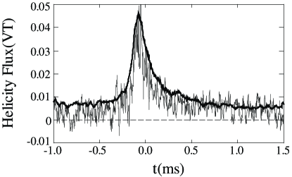
Figure 15: Time evolution of measured helicity flux (thin line) due to MHD dynamo effects compared to the prediction (thick line) from the helicity balance during a relaxation event [14].

The helicity flux has been measured directly for the same plasma shown in Fig. 11 at $r=b\equiv a-5$cm. All other five terms in Eq. (23) were determined independently. As shown in Fig. 15, the measured outward helicity flux due to MHD dynamo can exactly account for helicity change in $K_{\rm edge}$ and $K_{\rm link}$, demonstrating the existence of a helicity flux associated with fast dynamos observed in RFP plasmas. We note that the quasi-steady state of the plasma is maintained by an inward helicity injection by the transformer via the third term of the surface integral of Eq. (20).

The requirement of helicity flow in a driven system for fast and unquenched dynamos has important implications to the physics of astrophysical dynamos [51, 52]. A good example under debate is the solar dynamo, which is driven by a combination of thermal gradient and rotation. It has been found that there is a preference in the sign of the observed twisted field lines (hence the helicity) in each hemisphere [53, 54] and consequently in the solar wind [55]. This helicity preference may well be a result of helicity flow accompanied with the solar dynamo, which must be fast and unquenched to explain the observed 11 year solar cycle. If the electrostatic MHD dynamo is operational like in laboratory plasmas, there are two possible explanations. The first possibility [46] is that the fast dynamo actions transport or separate the large-scale helicity of one sign to one hemisphere while leaving the opposite helicity in the other hemisphere. Then they rise to the solar surface via buoyancy. The second possibility [51] is that the fast dynamo produces a helicity flow from the convection zone to the surface to drive the corona. The sign of the helicity is different at each hemisphere due to opposite signs of the $\alpha$ effect. Both mechanisms conserve the total helicity. These large-scale structures and its associated helicity are constantly removed from the solar surface by flaring. Both mechanisms can also replace the lost helicity continuously.

6. Conclusions

The physics of the $\alpha$ effects measured in the pinch plasmas has been reviewed, largely based on simple, intuitive approaches. It has been demonstrated that the observed dynamo effects are part of magnetic self-organization processes, either continuous or discrete in time. MHD dynamo and diamagnetic dynamo have been successfully measured and there is supporting evidence on Hall dynamo and kinetic dynamo. The close relationship with the concept of magnetic helicity has been studied, and it has been directly measured that the dynamo activity is accompanied by an outward helicity flow.

Implications of these measurements and understanding have been discussed in the context of astrophysical dynamos. Despite important differences in the form of the driving free energy, dynamos in laboratory plasmas exhibit remarkable similarities with the required astrophysical dynamos: they are fast (operational at small resistivity) and unquenched (operational in a large mean field). It has been shown that these desired features cannot exist in the traditionally assumed stationary and homogeneous turbulence. In fact, both the laboratory plasmas and astrophysical dynamos are driven systems which invalidate the stationarity and/or homogeneity assumption on the generated turbulence, thus allowing fast and unquenched dynamos to function. Despite several caveats, the availability of laboratory plasmas provides a unique and useful testbed to enhance understanding of astrophysical problems, such as dynamo.

• Received

REFERENCES

- [1] E.N. Parker. Cosmical Magnetic Fields. Clarendon Press, Oxford, (1979).
- [2] H.K. Moffatt. Magnetic Field Generation in Electrically Conducting Fluids Cambridge University Press, Cambridge, (1978).
- [3] F. Krause and K.-H. Rädler. Mean-Field Magnetohydrodynamics and Dynamo Theory. Akademie-Verlag, Berlin, (1980).
- [4] H.A.B. Bodin and A.A. Newton. Reversed-Field-Pinch Research. Nuclear Fusion, vol. 20 (1980), pp. 1255–1324.
- [5] H.A.B. Bodin. The Reversed Field Pinch. Nuclear Fusion, vol. 30 (1990), pp. 1717–1737.
- [6] T.R. Jarboe. Review of Spheromak Research. Plasma Phys. Controlled Fusion, vol. 36 (1994), pp. 945–990.
- [7] P.M. Bellan. Spheromaks. Imperial College Press, London, (2000).
- [8] E.J. Caramana and D.A. Baker. The Dynamo Effect in Sustained Reversed-Field Pinch Discharges. Nuclear Fusion, vol. 24 (1984), pp. 423–434.
- [9] S. Ortolani and D.D. Schnack. Magnetohydrodynamics of Plasma Relaxation. World Scientific Publishing Co., Singapore, (1993).
- [10] J.B. Taylor. Relaxation and Magnetic Reconnection in Plasmas. Rev. Mod. Phys., vol. 58 (1986), pp.741.
- [11] R. Watt and R. Nebel. Sawteeth, Magnetic Disturbances, and Magnetic Flux Regeneration in the Reversed-Field Pinch. Phys. Fluids, vol. 26 (1983), pp.2268.
- [12] S.A. Hokin, A. Almagri, S. Assadi, J. Beckstead, G. Chartas, N. Crocker, M. Cudzinovic, D. Den Hartog, R. Dexter, D. Holly, S. Prager, T. Rempel, J. Sarff, E. Scime, W. Shen, C. Spragins, C. Sprott, G. Starr, M. Stoneking, C. Watts, R. Nebel. Global Confinement and Discrete Dynamo Activity in the MST Reversed-Field Pinch. Phys. Fluids B, vol. 3 (1991), pp.2241.
- [13] M. Yamada. Study of Magnetic Helicity and Relaxation Phenomena in Laboratory Plasmas. Magnetic Helicity in Space and Laboratory Plasmas, AGU Geophysical Monograph 111 (1999), pp.129–140.
- [14] H. Ji, S.C. Prager, and J.S. Sarff. Conservation of Magnetic Helicity during Plasma Relaxation. Phys. Rev. Lett., vol. 74 (1995), pp.2945–2948.
- [15] H.P. Furth, J. Killeen, and M.N. Rosenbluth. Finite-Resistivity Instabilities of a Sheet Pinch. Phys. Fluids, vol. 6 (1963), pp.459–484.
- [16] H.R. Strauss. The Dynamo Effect in Fusion Plasmas. Phys. Fluids, vol. 28 (1985), pp.2786–2792.
- [17] A. Bhattacharjee and E. Hameiri. Self-Consistent Dynamolike Activity in Turbulent Plasmas. Phys. Rev. Lett., vol. 57 (1986), pp.206–209.
- [18] H. Ji, H. Toyama, A. Fujisawa, S. Shinohara, and K. Miyamoto. Fluctuations and Edge-current Sustainment in a Reversed-Field Pinch. Phys. Rev. Lett., vol. 69 (1992), pp.616–619.
- [19] H. Ji, H. Toyama, K. Yamagishi, S. Shinohara, A. Fujisawa, and K. Miyamoto. Probe Measurements in the REPUTE-1 Reversed Field Pinch. Rev. Sci. Instrum., vol. 62 (1991), pp. 2326–2337.
- [20] H. Ji, A.F. Almagri, S.C. Prager, and J.S. Sarff. Time-resolved Observation of Discrete and Continuous MHD Dynamo in the Reversed-Field Pinch Edge. Phys. Rev. Lett., vol. 73 (1994), pp.668–671.
- [21] A. al-Karkhy, P.K. Browning, G. Cunningham, S.J. Gee, and M.G. Rusbridge. Observations of the Magnetohydrodynamic Dynamo Effect in a Spheromak Plasma. Phys. Rev. Lett., vol. 70 (1993), pp.1814–1817.
- [22] D.J. Den Hartog, J.T. Chapman, D. Craig, G. Fiksel, P.W. Fontana, and S.C. Prager. Measurement of Core Velocity Fluctuations and the Dynamo in a Reversed-Field Pinch. Phys. Plasmas, Vol. 6 (1998), pp.1813–1821.
- [23] P.W. Fontana, D.J. Den Hartog, G. Fiksel, and S.C. Prager. Spectroscopic Observation of Fluctuation-Induced Dynamo in the Edge of the Reversed-Field Pinch. Phys. Rev. Lett., vol. 85 (2000), pp.566–569.
- [24] G. Fiksel, D.J. Den Hartog, and P.W. Fontana. An Optical Probe for Local Measurements of Fast Plasma Ion Dynamics. Rev. Sci. Instrum., vol. 69 (1998), pp. 2024–2026.
- [25] H. Ji, Y. Yagi, K. Hattori, A.F. Almagri, S.C. Prager, Y. Hirano, J.S. Sarff, T. Shimada, Y. Maejima, and K. Hayase. Effect of Collisionality and Diamagnetism on the Plasma Dynamo. Phys. Rev. Lett., vol. 75 (1995), pp.1086–1089.
- [26] H. Ji, S.C. Prager, A.F. Almagri, J.S. Sarff, Y. Yagi, Y. Hirano, K. Hattori, and H. Toyama. Measurements of the Dynamo Effect in a Plasma. Phys. Plasmas, vol. 3 (1996), pp.1935–1942.
- [27] R.A. Nebel. Two-Fluid Simulations of the Reversed-Field Pinch. Las Alamos National Laboratory Report LA-UR-90-3534, (1990).
- [28] W. Shen and S.C. Prager. The Fluctuation-Induced Hall Effect. Phys. Fluids B, vol. 5 (1993), pp.1931–1933.
- [29] A.R. Jacobson and R.W. Moses. Nonlocal DC Electric Conductivity of a Lorentz Plasma in a Stochastic Magnetic Field. Phy. Rev. A, vol. 29 (1984), pp. 3335–3342.
- [30] J.C. Ingraham, R.F. Ellis, J.N. Downing, C.P. Munson, P.G. Weber, and G.A. Wurden. Engergetic Electron Measurements in the Edge of a Reversed-Field Pinch. Phys. Fluids B, vol. 2 (1990), pp.143–159.
- [31] P.W. Terry and P.H. Diamond. A Self-Consistent Theory of Radial Transport of Field-Aligned Current by Microturbulence. Phys. Fluids B, vol. 2 (1990), pp.1128–1137.
- [32] Y. Yagi, G. Serianni, H. Ji, and Y. Maejima. Correlation Studies on Fast Electrons and Dynamo-Related Activities in a Reversed-Field Pinch Plasma. Jpn. J. Appl. Phys., vol. 38 (1999), pp.4213–4225.
- [33] N. Seehafer. The Turbulent Electromotive Force in the High-Conductivity Limit. Astron. Astrophys., vol. 301 (1995), pp.290–292.
- [34] R.M. Kulsrud and S.W. Anderson. The Spectrum of Random Magnetic Fields in the Mean Field Dynamo Theory of the Galactic Magnetic Field. Astrophys. J., vol. 396 (1992), pp.606–630.
- [35] A.V. Gruzinov and P.H. Diamond. Self-Consistent Theory of Mean-Field Electrodynamics. Phys. Rev. Lett., vol. 72 (1992), pp.1651–1653.
- [36] A. Bhattacharjee and Y. Yuan. Self-Consistency Constraints on the Dynamo Mechanism. Astrophys. J., vol. 449 (1995), pp.739–744.
- [37] S. Vainshtein. Exactly Solvable Model of Nonlinear Dynamo. Phys. Rev. Lett., vol. 80 (1998), pp.4879–4882.
- [38] F. Cattaneo and D.W. Hughes. Nonlinear Saturation of the Turbulent Effect. Phys. Rev. E, vol. 54 (1996), pp.R4532-R4535.
- [39] A. Pouquet, U. Frisch, and J. Leorat. Strong MHD Helical Turbulence and Nonlinear Dynamo Effect J. Fluid Mech., vol. 77 (1976), pp.321–354.
- [40] S.C. Prager. Helicity, Relaxation, and Dynamo in a Laboratory Plasma. Magnetic Helicity in Space and Laboratory Plasmas, AGU Geophysical Monograph 111 (1999), pp.55–63.
- [41] R.L. Stenzel and W. Gekelman. Experiments on Magnetic-Field-Line Reconnection. Phys. Rev. Lett., vol. 42 (1979), pp.1055–1057.
- [42] A. Brandenburg. The Inverse Cascade and Nonlinear Alpha-Effect in Simulations of Isotropic Helicical Hydromagnetic Turbulence. Astrophys. J., vol. 550 (2001), pp.824–840.
- [43] E.G. Blackman and G.B. Field. Constraints on the Magnitude of in Dynamo Theory. Astrophys. J., vol. 534 (2000), pp.984–988.
- [44] A. Brandenburg and J. Donner. The Dependence of the Dynamo Alpha on Vorticity. Mon. Not. Roy. Astron. Soc., vol. 288 (1996), pp.L29–L33.
- [45] A. Brandenburg and W. Dobler. Large Scale Dynamo with Helicity Loss through Boundaries. Astron. Astrophys., vol. 368 (2001), pp.329–338.
- [46] H. Ji. Turbulent Dynamos and Magnetic Helicity. Phys. Rev. Lett., vol. 83 (1999), pp.3198–3201.
- [47] A.H. Boozer. Ohm’s Law for Mean Magnetic Field. J. Plasma Phys., vol. 35 (1986), pp.133-139.
- [48] E. Hameiri and A. Bhattacharjee. Turbulence Magnetic Diffusion and Magnetic Field Reversal. Phys. Fluids, vol. 30 (1987), pp.1743–1755.
- [49] T. Stribling and W.H. Matthaeus. Statistical Properties of Ideal Three-Dimensional Magnetohydrodynamics. Phys. Fluids B, vol. 2 (1990), pp.1979–1988.
- [50] M.K. Bevir and J.W. Gray. Relaxation, Flux Consumption and Quast Steady State Pinches. Proc. Reversed-Field Pinch Theory Workshop, Los Alamos (1981), Report No. LA-8944-C, pp.176–180.
- [51] E.G. Blackman and G.B. Field. Coronal Activity from Dynamo in Astrophysical Rotators. Mon. Not. Roy. Astron. Soc., vol. 318 (2000), pp.724–732.
- [52] E.T. Vishniac and J. Cho. Magnetic Helicity Conservation and Astrophysical Dynamos. Astrophys. J., vol. 550 (2001), pp.752–760.
- [53] D.M. Rust and A. Kumar. Helical Magnetic Fields in Filaments. Solar Phys., vol. 155 (1994), pp.69–97.
- [54] A.A. Pevtsov, R.C. Canfield, and T.R. Metcalf. Latitudinal Variation of Helicity of Photospheric Magnetic Fields. Astrophys. J., vol. 440 (1995), pp.L109–L112.
- [55] D.M. Rust. Spawning and Shedding Helical Magnetic Fields in the Solar Atmosphere. Geophys. Res. Lett., vol. 21 (1994), pp.241–244.
-