New physics and astronomy with the new gravitational-wave observatories

Abstract

Gravitational-wave detectors with sensitivities sufficient to measure the radiation from astrophysical sources are rapidly coming into existence. By the end of this decade, there will exist several ground-based instruments in North America, Europe, and Japan, and the joint American-European space-based antenna LISA should be either approaching orbit or in final commissioning in preparation for launch. The goal of these instruments will be to open the field of gravitational-wave astronomy: using gravitational radiation as an observational window on astrophysics and the universe. In this article, we summarize the current status of the various detectors currently being developed, as well as future plans. We also discuss the scientific reach of these instruments, outlining what gravitational-wave astronomy is likely to teach us about the universe.

I Introduction

A common misconception outside of the gravitational-wave research community is that the primary purpose of observatories such as LIGO is to detect directly gravitational waves. Although the first unambiguous direct detection will certainly be a celebrated event, the real excitement will come when gravitational-wave detection can be used as an observational tool for astronomy. Because the processes which drive gravitational-wave emission are fundamentally different from processes that radiate electromagnetically, gravitational-wave astronomy will provide a view of the universe that is rather different from our “usual” views.

Because they arise from fundamentally different physical processes, the information carried by gravitational radiation is “orthogonal” to that carried by electromagnetic radiation. Consider the following differences:

• Electromagnetic waves are oscillations of electric and magnetic fields that propagate through spacetime. Gravitational waves are oscillations in spacetime itself.

• Astrophysical electromagnetic radiation typically arises from the incoherent superposition of emissions from individual electrons, atoms, and molecules. They often provide direct information about the thermodynamic state of a system or environment. Gravitational waves are coherent superpositions of radiation that arise from the bulk dynamics of a dense source of mass-energy (matter or highly curved spacetime). They provide direct information about the system’s dynamics.

• The wavelength of electromagnetic radiation is typically smaller than the radiating system. They can thus be used to form an image of that system; any good public lecture on astronomy includes a number of “pretty pictures”. By contrast, the wavelength of gravitational radiation is typically of order or larger than the size of the radiating source. Such waves cannot be used to image the source; instead, the two gravitational-wave polarizations are akin to sound, carrying a stereophonic description of the source’s dynamics. Indeed, it is becoming common for workers in gravitational radiation to play audio encodings of expected gravitational-wave events, and the notion of “pretty sounds” (or at least “interesting sounds”) may become widely accepted as gravitational-wave astronomy matures.

• With a few exceptions, electromagnetic astronomy is based upon deep imaging of narrow, small-angle fields of view: observers obtain a large amount of information about sources on a small piece of the sky. Gravitational-wave astronomy will be an all-sky affair: observatories such as LIGO and LISA have nearly $4\pi$ steradian sensitivity to events over the sky. A consequence of this is that their ability to localize a source’s sky position is not good by usual astronomical standards; but, it means that any source on the sky will be detectable, not just sources towards which the instrument is “pointed”. The contrast between the all-sky sensitivity, relatively poor angular resolution of gravitational-wave observatories, and the pointed, high angular resolution of telescopes is very similar to the angular resolution contrast of hearing and sight, strengthening the useful analogy of gravitational waves with sound.

• Electromagnetic waves interact strongly with matter; gravitational-waves do not. This is both blessing and curse: it means that gravitational waves propagate from emission to Earth with essentially zero absorption, making it possible to probe astrophysics that is hidden or dark (for example, the coalescence and merger of black holes; the collapse of a stellar core; the dynamics of the early universe very soon after the big bang). It also means that the waves interact very weakly with gravitational-wave detectors, requiring enormous experimental effort for assured detection.

• The directly observable gravitational waveform $h$ is a quantity that falls off as $1/r$. Most electromagnetic observables are some kind of energy flux, and so fall off with distance with a $1/r^{2}$ law. Because of this, relatively small improvements in the sensitivity of gravitational-wave detectors have an enormous impact on their ability to make measurements: doubling a detector’s sensitivity doubles the distance to which sources can be detected, increasing the volume of the universe in which sources are measurable by a factor of eight. Every factor of two improvement in the sensitivity of a gravitational-wave observatory increases the number of observable sources by nearly an order of magnitude.

These differences motivate the efforts to inaugurate gravitational-wave astronomy as a vital field. In this article, we will describe current efforts to develop ground-based detectors (Sec. III, focusing in particular on the American LIGO project) as well as the joint American-European space-based LISA project (Sec. IV). We also discuss in some detail the science that can be expected from gravitational-wave astronomy (Sec. V). First, we briefly discuss the properties of gravitational waves and their likely strength, and sketch how a gravitational-wave detector is able to measure their tiny effects.

II Gravitational waves and detectors: overview

Gravitational radiation is a natural consequence of general relativity (indeed, of any causal theory of gravitation; see dank_thesis for a fascinating discussion of early work by Laplace on gravitation with a finite speed of propagation). It was first described more-or-less correctly by Albert Einstein in 1918 bigal1 . (In an earlier work bigal2 , Einstein predicted gravitational radiation, though with a rather incorrect description.) General relativity describes the radiation as a tensor perturbation to the metric of spacetime (so that it can be thought of as a spin-2 boson), propagating at the speed of light, and with two independent polarizations.

As electromagnetic radiation is generated by the acceleration of charges, gravitational radiation arises from the acceleration of masses. In particular, electromagnetic waves are created (at lowest order) by the time changing charge dipole moment, and are thus dipole waves. Monopole EM radiation would violate charge conservation. At lowest order, gravitational waves come from the time changing quadrupolar distribution of mass and energy; monopole gravitational waves would violate mass-energy conservation, and dipole waves violate momentum conservation.

Gravitational waves act tidally, stretching and squeezing any object that they pass through. Because the waves arise from quadrupolar oscillations, they are themselves quadrupolar in character, squeezing along one axis while stretching along the other. When the size of the object that the wave acts upon is small compared to the wavelength (as is the case for LIGO), forces that arise from the two GW polarizations act as in Fig. 1. The polarizations are named “$+$” (plus) and “$\times$” (cross) because of the orientation of the axes associated with their force lines.

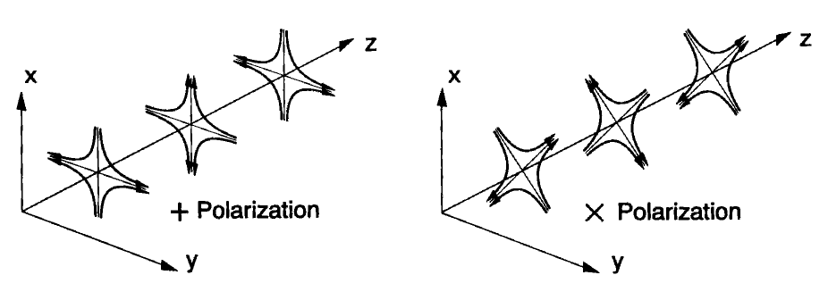
Figure 1: The lines of force associated with the two polarizations of a gravitational wave (from Ref. ligoscience ).

Interferometric gravitational-wave detectors measure this tidal field by measuring their action upon a widely-separated set of test masses. In ground-based interferometers, these masses are arranged as in Fig. 2. The space-based detector LISA arranges its test masses in a large equilateral triangle that orbits the sun, illustrated in Fig. 3. On the ground, each mass is suspended with a sophisticated pendular isolation system to eliminate the effect of local ground noise. Above the resonant frequency of the pendulum (typically of order $1\,{\rm Hz}$), the mass moves freely. (In space, the masses are actually free floating.) In the absence of a gravitational wave, the sides $L_{1}$ and $L_{2}$ shown in Fig. 2 are about the same length $L$.

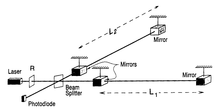
Figure 2: Layout of an interferometer for detecting gravitational waves (from Ref. ligoscience ).

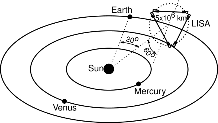
Figure 3: Orbital configuration of the LISA antenna.

Suppose the interferometer in Fig. 2 is arranged such that its arms lie along the $x$ and $y$ axes of Fig. 1. Suppose further that a wave impinges on the detector down the $z$ axis, and the axes of the $+$ polarization are aligned with the detector. The tidal force of this wave will stretch one arm while squeezing the other; each arm oscillates between stretch and squeeze as the wave itself oscillates. The wave is thus detectable by measuring the separation between the test masses in each arm and watching for this oscillation. In particular, since one arm is always stretched while the other is squeezed, we can monitor the difference in length of the two arms:

$$\delta L(t)\equiv L_{1}(t)-L_{2}(t)\;.$$ (1)

For the case discussed above, this change in length turns out to be the length of the arm times the $+$ polarization amplitude:

$$\delta L(t)=h_{+}(t)L\;.$$ (2)

The gravitational wave acts as a strain in the detector; $h$ is often referred to as the “wave strain”. Note that it is a dimensionless quantity. Aficionados of general relativity can easily derive Eq. (2) by applying the equation of geodesic deviation to the separation of the test masses and using a gravitational-wave tensor on a flat background spacetime to develop the curvature tensor; see Ref. 300yrs , Sec. 9.2.2 for details. We obviously do not expect astrophysical gravitational-wave sources to align themselves in as convenient a manner as described above. Generally, both polarizations of the wave influence the test masses:

$${\delta L(t)\over L}=F^{+}h_{+}(t)+F^{\times}h_{\times}(t)\equiv h(t)\;.$$ (3)

The antenna response functions $F^{+}$ and $F^{\times}$ weight the two polarizations in a quadrupolar manner as a function of a source’s position and orientation relative to the detector; see 300yrs , Eqs. (104a,b) and associated text.

In ground-based interferometers, the test masses at the ends of each arm are made of a highly transparent material (fused silica in present designs; perhaps sapphire in future upgrades). The mirrors at the far end of each arm have amplitude reflectivities approaching unity. The mirrors at the corner are less reflective since they must couple the light into the Fabry-Perot cavity arms. The corner mirrors’ multilayer dielectric coatings have power reflectivities $T\sim 3\%$. A very stable laser beam is divided at the beamsplitter, directing light into the two arm cavities. If the finesse of the cavity is ${\cal F}$ and the amplitude reflectivity of the corner mirrors is $r_{\rm corner}$, then each photon makes on average ${\cal F}/\pi\simeq\sqrt{r_{\rm corner}}/(1-r_{\rm corner})\sim 65$ bounces. The light from the two arms then recombines at the beamsplitter. The mirrors are positioned so that, in the absence of a gravitational wave, all of the light goes back towards the laser and the photodiode reads no signal. If a signal is present, the relative phase $\Phi$ of the two beams changes by an amount proportional to $h$, changing the light’s interference pattern. Without any intervention, this would cause light to leak into the photodiode. In principle, the wave strain $h$ could be read from the photointensity of this light. In practice, a system of servo loops controls the system such that destructive interference is guaranteed — the photodiode is kept dark, and so is called the “dark port”. The wave strain $h$ is then encoded in the servo signals used to keep the dark port dark.

The wave strain must fall off with distance as a $1/r$ law to conserve the total energy flowing through large spheres. We have already argued that the lowest order contribution to the waves is due to the changing quadrupole moment of the source. To order of magnitude, this moment is given by $Q\sim(\mbox{source mass})(\mbox{source size})^{2}$. By dimensional analysis, we then know that the wave strain must have the form

$$h\sim{G\over c^{4}}{\ddot{Q}\over r}\;.$$ (4)

The second time derivative of the quadrupole moment is given approximately by $\ddot{Q}\simeq 2Mv^{2}\simeq 4E^{\rm ns}_{\rm kin}$; $v$ is the source’s internal velocity, and $E^{\rm ns}_{\rm kin}$ is the nonspherical part of its internal kinetic energy. Strong sources of gravitational radiation are sources that have strong non-spherical dynamics — for example, compact binaries (containing white dwarfs, neutron stars, and black holes), mass motions in neutron stars and collapsing stellar cores, the dynamics of the early universe. In order to have an interesting rate of observable events, we need to be sensitive to sources at rather large distances. For example, when binary neutron stars coalesce, we need to reach out to several hundred Mpc (i.e., a substantial fraction of $10^{9}$ light years) nps ; phinney91 ; kalogera_lorimer . In such a case $E^{\rm ns}_{\rm kin}/c^{2}\sim\mbox{1 solar mass}\,(\equiv 1\,M_{\odot})$. Plugging these numbers into Eq. (4) yields the estimate

$$h\sim 10^{-21}-10^{-22}\;.$$ (5)

This sets the sensitivity required to measure gravitational waves. Combining this scale with Eq. (3) says that for every kilometer of baseline $L$, we need to be able to measure a distance shift $\delta L$ of better than $10^{-16}$ centimeters.

The prospect of achieving such a stringent displacement sensitivity often strikes people as insane. How can light whose wavelength $\lambda\sim 10^{-4}\,{\rm cm}$ is $10^{12}$ times larger than the typical displacement be used to measure that displacement? For that matter, how is it possible that thermal motions do not wash out such a tiny effect?

That such measurement is possible with laser interferometry was analyzed thoroughly and published by Rainer Weiss in 1972 weiss72 . (It should be noted that the possibility of detecting gravitational waves with laser interferometers has an even longer history, reaching back to Pirani in 1956, and has been independently invented by several workers: Gertsenshtein and Pustovoit in 1962, Weber in the 1960s, and Weiss c. 1970. See Sec. 9.5.3 of Ref. 300yrs for further discussion and references.) Examine first how the 1 micron laser can measure a $10^{-16}$ cm effect. As mentioned above, the light bounces roughly 100 times before leaving the arm cavity (corresponding to about half a cycle of a 100 Hz gravitational wave). The light’s acquired phase shift during those 100 round trips is

$$\Delta\Phi_{\rm GW}\sim 100\times 2\times\Delta L\times 2\pi/\lambda\sim 10^{-9}\;.$$ (6)

This phase shift can be measured provided that the photon shot noise at the photodiode, $\Delta\Phi_{\rm shot}\sim 1/\sqrt{N}$, is less than $\Delta\Phi_{\rm GW}$. $N$ is the number of photons accumulated over the measurement; $1/\sqrt{N}$ is the magnitude of phase fluctuation in a coherent state, appropriate for describing a laser. We therefore must accumulate $10^{18}$ photons over the roughly $0.01$ second measurement, which translates to a laser power of about 100 watts. In fact, as was pointed out by Ron Drever drever_recycle , one can use a much less powerful laser: even in the presence of a gravitational wave, only a tiny portion of the light that comes out of the interferometer’s arms goes to the photodiode. The vast majority of the laser power is sent back to the laser. An appropriately placed mirror bounces this light back into the arms, recycling the laser light. The recycling mirror is shown in Fig. 2, labeled “R”. With it, a laser of $\sim 10$ watts drives several hundred watts to circulate in the “recycling cavity” (the optical cavity between the recycling mirror and the arms), and $\sim 10$ kilowatts to circulate in the arms.

Thermal excitations are overcome by averaging over many many vibrations. For example, the atoms on the surface of the interferometers’ test mass mirrors oscillate with an amplitude

$$\delta l_{\rm atom}=\sqrt{kT\over m\omega^{2}}\sim 10^{-10}\,{\rm cm}$$ (7)

at room temperature $T$, with $m$ the atomic mass, and with a vibrational frequency $\omega\sim 10^{14}\,{\rm s}^{-1}$. This amplitude is huge relative to the effect of the gravitational wave — how can we possibly hope to measure the wave? The answer is that atomic vibrations are random and incoherent. The $\sim 7$ cm wide laser beam averages over about $10^{17}$ atoms and at least $10^{11}$ vibrations in a typical measurement. Atomic vibrations are irrelevant compared to the coherent effect of a gravitational wave. Other thermal vibrations, however, are not irrelevant and in fact dominate the noise spectrum of LIGO in certain frequency bands. For example, the test masses’ normal modes are thermally excited. The typical frequency of these modes is $\omega\sim 10^{5}\,{\rm s}^{-1}$, and they have mass $m\sim 10\,{\rm kg}$, so $\delta l_{\rm mass}\sim 10^{-14}\,{\rm cm}$. This, again, is much larger than the effect we wish to observe. However, the modes are very high frequency, and so can be averaged away provided the test mass is made from material with a very high quality factor $Q$. Understanding the physical nature of noise in gravitational-wave detectors is an active field of current research; see Refs. levin ; liu_thorne ; santamore_levin ; buonanno_chen ; hughes_thorne ; tcreighton and references therein for a glimpse of recent work. In all cases, the fundamental fact to keep in mind is that a gravitational wave acts coherently, whereas noise acts incoherently, and thus can be beaten provided one is able to average away the incoherent noise sources.

III Ground-based detectors

The first generation of long baseline, kilometer-scale interferometric gravitational-wave detectors are being constructed and commissioned at several sites around the world. Briefly, the major ground-based interferometric gravitational-wave projects are as follows:

• LIGO. Three LIGO interferometers are in the commissioning phase: two in Hanford, Washington (with 2 and 4 km arms, sharing the vacuum system), and one in Livingston, Louisiana (4 km arms). An aerial view of the Hanford site is included in Fig. 4. The LIGO detectors are designed to operate in the power recycled Michelson configuration with arms acting as Fabry-Perot cavities. The large distance between sites (about $3000$ km) and differing arm lengths are designed to support coincidence analysis. Much current research and development is focused on Advanced LIGO detector design. The new generation of detectors will provide a broader frequency band and a $\sim$ 10-fold increase in range for inspiral sources via the lowered noise floor.

• Virgo. Virgo, the Italian/French long baseline gravitational-wave detector, is under construction near Pisa, Italy marion2000 . It has 3 km arms and advanced passive seismic isolation systems. In most respects, Virgo is very similar to LIGO; a major difference is that it should achieve better low frequency sensitivity from the beginning due to its advanced seismic isolation system. Virgo will very usefully complement the LIGO detectors, strengthening coincidence analysis and making source position determination possible.

• GEO600. GEO600 is a 600 meter interferometer being built by a British-German collaboration in the vicinity of Hannover, Germany luck2000 . It will use advanced interferometry and advanced low noise multiple pendulum suspensions, serving as a testbed for advanced detector technology and allowing it to achieve sensitivity comparable to the multi-kilometer instruments.

• TAMA300. The TAMA detector near Tokyo, Japan can already claim significant observation time with more than 1000 hours of operation andoetal . It has achieved a peak strain sensitivity of $h\sim 10^{-20}\,{\rm Hz}^{-1/2}$ explain_sensitivity at frequencies near 1000 Hz. TAMA has 300 meter arms and is operated in the recombined Michelson configuration with Fabry-Perot arms. A much improved 3 km detector is currently under design kuroda2000 .

• ACIGA. The Australian Consortium for Interferometric Gravitational Astronomy plans to build an observatory near Perth, Australia mccleland2000 . They are presently engaged in the construction of an 80 meter research interferometer, which can be extended to kilometer scale. They are studying advanced detection methods and technologies which could lead to much decreased noise floors in advanced ground based interferometers.

Since interferometric gravitational-wave detectors are sensitive to nearly all directions, it is nearly impossible to deduce pointing information from the signal of a single detector. To get accurate information about the source direction it is necessary to make use of the detection time difference among detectors. These detectors must be widely spaced and not collinear. At the very minimum, three sites are needed for acceptable pointing. A fourth detector, widely removed from the plane of the other three, is particularly valuable for improving directional information. Thus a detector in Australia would greatly add to the science output of the gravitational-wave observatory network, which is otherwise confined entirely to the northern hemisphere.

LIGO is a good example to illustrate the design and operation principles of kilometer-scale interferometers; we shall focus on it for the remainder of our discussion.

III.1 LIGO overview

Construction of both LIGO facilities and vacuum systems was completed by early 2000. The 2 km interferometer at the Hanford site was installed in mid 2000; the Livingston site 4 km interferometer was finished by late 2000. Installation of the Hanford 4 km interferometer was delayed due to repairs needed following the February 28, 2001 earthquake; as this document is being written, installation is well underway. Both observatories are concentrating on detector commissioning and a series of “Engineering Runs”. These Runs have provided excellent real life experience for the participating members of the LIGO Scientific Community, paving the way for the approaching “Science Run” scheduled to begin at the end of 2001. This will be followed by more frequent and longer Science Runs until 2006, when major detector upgrades are scheduled. In parallel to the commissioning effort and Engineering/Science Runs, the collaboration also focuses on the research and development of advanced LIGO detectors, promising a wider detector band and greatly improved sensitivity.

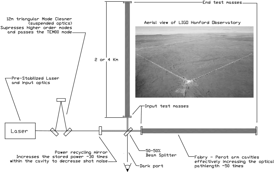
Figure 4: Simplified optical layout of a LIGO interferometer. Shown here are the prestabilized laser, the input mode cleaner, the recycling mirror, and the test mass mirrors. As discussed in Sec. II, servo loops ensure that the recombined light destructively interferes so that the dark port is kept dark. The gravitational wave signal is read out from the forces needed to keep the recombined light in destructive interference.

The LIGO detectors operate as power recycled Michelson interferometers with Fabry-Perot arms; see Fig. 4. Very high duty cycle is needed for each interferometer in order to effectively use the full network for coincidence analysis, which is necessary to achieve a low false detection rate and have high confidence in observations. The wide (3000 km) separation between the LIGO sites is large enough that the chance of environmentally induced coincidence events is negligible. Both sites are heavily equipped with environmental sensors that thoroughly cover a wide range of possible disturbances that could cause false detections. For example, LIGO monitors the local seismic background, electromagnetic fluctuations, acoustic noise, cosmic radiation, dust, vacuum status, weather, records power line transients, and uses ultra-sensitive magnetometers at several locations at each observatory.

We now briefly describe the operating principles of LIGO optics, the major sources of noise that limit sensitivity, the data analysis system that will be used during operations, and plans for future upgrades.

III.1.1 Laser, optics and configuration

The basic optical layout of the LIGO detectors is shown in Figure 4. LIGO uses a Nd:YAG near infrared laser (wavelength 1064 nm) with peak power $\sim$ 10W as the light source. Various electro-optical components and servo loops are used to stabilize both the frequency and power of the laser.

The light from the pre-stabilized laser passes through the input optics and is coupled into the 12 meter, triangular mode cleaner cavity. The mode cleaner passes only the TEM₀₀ mode, eliminating higher order modes. Starting with the mode cleaner, every major optical component is within a large vacuum system, capable of reaching $10^{-9}$ Torr. After conditioning by the mode cleaner, the light enters the interferometer. All major optics in the interferometer are suspended on a single steel wire loop, mechanically isolated from the ground by vibration isolators and controlled by multiple servo loops. The mirrors are made of fused silica with extremely high mechanical $Q$ and are polished to within $\sim$ 1 nanometer RMS. They have high homogeneity, low bulk loss and multi-layer coatings with less than 50 ppm scattering loss. Each mirror is actuated by four precision coils, each positioned around a permanent magnet glued to the back side of the test masses. The coil assembly also features a sensitive shadow sensor for local control. Additional optical levers and wavefront sensors provide more precise sensing. The laser beam is coupled into the arms by a beam splitter. Each arm is a Fabry-Perot optical cavity, increasing the effective length of the arm to magnify the phase shift (proportional to cavity finesse) caused by the wave. The stored power within the interferometer is built up by the partially transmitting recycling mirror.

An operating interferometer tries to keep the dark port perfectly dark, holding the various optical components such that light coming out of the arms destructive interferes and no light goes to the photodetector. When this is achieved, the interferometer is on resonance, with maximum power circulating in the arms. Several interconnected control loops are used to achieve and then maintain resonance. An interferometer on resonance is usually described as locked. Keeping lock must be highly automated, requiring minimal operator interaction for high uptime. The gravitational-wave signal is extracted from the servo signals used to maintain the lock and correct for the length difference between the arms.

III.1.2 Noise sources

Gravitational-wave interferometers have their sensitivity limited by a number of noise sources. We list here some of the most important and interesting fundamental noise sources; many of these were recognized and had their magnitude estimated by Rainer Weiss in 1972 weiss72 .

• Seismic noise. Ambient or culturally induced seismic waves continuously pass under the test masses of the detector. The natural motion of the surface peaks around 150 mHz; this is called the “microseismic peak”. Cultural noises tend to be at higher frequencies, near several Hz. The test masses must be carefully isolated from the ground to effectively mitigate the seismic noise. Seismic noise will limit the low frequency sensitivity of first generation ground-based gravitational-wave detectors.

• Thermal noise. Thermally excited vibrational modes of the test mass or the suspension system will couple into the resonances of the system. By improving the $Q$ of the components one can decrease the thermally induced noise between resonances.

• Shot noise. The number of photons in the input laser beam fluctuates; this surfaces as noise at the dark port. The strain noise due to this effect is proportional to $1/\sqrt{\mbox{(recycling gain)(input laser power)}}$. Thus, increasing the recycling gain and/or increasing the laser power lowers the shot noise. Unfortunately, high power in the cavities induces other unwanted effects such as radiation pressure noise (discussed in the next item) or thermal lensing (local deformation of the optical surfaces of the cavity). The right choice of laser power and recycling gain is a compromise.

• Radiation pressure noise. Fluctuating number of photons bouncing from the mirrors will introduce a fluctuating force on the mirror. This effect is proportional to $\sqrt{\mbox{(recycling gain)(input laser power)}}$ — the inverse of the proportionality entering the shot noise. One cannot just increase the laser power without penalty. Reducing shot noise and radiation pressure noise in tandem is a topic of advanced detector R&D; techniques for doing so require specially prepared laser states. See buonanno_chen and references therein for further discussion.

• Gravity gradient noise. When seismic waves, atmospheric pressure fluctuations, cars, animals, tumbleweeds, etc., pass near a gravitational-wave detector, they act as density perturbations in the neighboring region. This in turn can produce significant fluctuating gravitational forces on the interferometer’s test masses hughes_thorne ; tcreighton . This is expected to become the limiting factor at low frequencies for advanced ground-based detectors with high quality seismic isolation systems.

• Laser intensity and frequency noise. The laser itself inevitably is somewhat noisy, with fluctuations in both intensity and frequency. This noise will not cancel out perfectly when the signal from the two arms destructively recombines, and so some noise can propagate into the signal on the dark port.

• Scattered light. Some laser light can scatter out of the main beam, and then be scattered back, coupling into the interferometer’s signal. This light will carry information about its scattering surface and be out of phase with the beam, and thus contaminate the desired signal. A dense baffling system has been installed to greatly reduce this source of noise.

• Residual gas. Any vacuum system contains some trace amount of gas that is extremely difficult to reduce; in LIGO, these traces (mostly hydrogen) are at roughly $10^{-9}$ Torr. Density fluctuations from these traces in the beam path will induce index of refraction fluctuations in the arms. Residual gas particles bouncing off the mirrors can also increase the displacement noise.

• Beam jitter. Jitter in the optics will cause the beam position and angle to fluctuate slightly, which causes some noise at the dark port.

• Electric fields. Fluctuations in the electric field around the test masses can couple into the interferometric signal via interaction between the field and the induced or parasitic surface charge on the mirror surface.

• Magnetic fields. Fluctuations in the local magnetic field can affect the test masses when interacting with the actuator magnets bonded to the surface of the mirrors.

• Cosmic showers. High energy penetrating muons can be stopped by the test masses and induce a random transient due to the recoil.

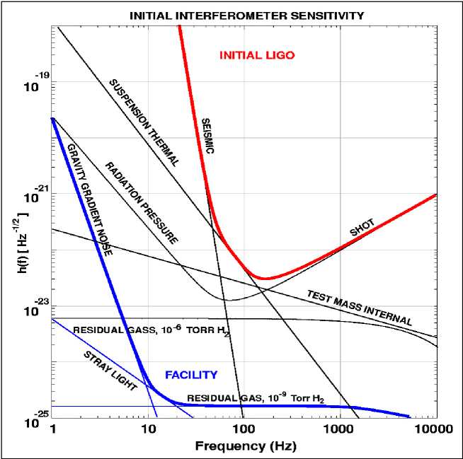
Figure 5: Illustration of LIGO sensitivity, showing the amplitude strain noise spectrum for various noise sources. The heavy line labeled “Initial LIGO” is the design goal for initial LIGO interferometers; that labeled “Facility” shows the facility limitations that cannot be avoided even if other noise sources are perfectly controlled.

The impact of the most important of these noise sources is shown in Fig. 5. The initial LIGO detectors will be limited by seismic noise at low frequencies ($\lesssim 50\,{\rm Hz}$), by thermal noise in the test mass suspensions at intermediate frequencies ($\sim 50-200\,{\rm Hz}$, and by shot noise at high frequencies ($\gtrsim 200\,{\rm Hz}$). The present detector noise is well above this target, particularly at low and intermediate frequencies.

As these noise sources are reduced, new challenges emerge. Eventually, any given instrument will be limited by a set of noise floors. The curve labeled “Facility Limit” in Fig. 5 sets the ultimate sensitivity that is likely to be attained even with all other noise sources controlled perfectly. At low frequencies, gravity gradient noise (which will be extremely difficult, if not impossible, to mitigate) will be the dominant source of noise; beyond that, optical path fluctuations from residual gas limit the sensitivity.

III.1.3 LIGO Data Analysis System (LDAS)

As will be discussed further below, the gravitational-wave datastream will be filtered by a large number ($\sim 10^{4}-10^{5}$) of model waveforms (“templates”) to search for sources such as coalescing compact binaries. These templates must be applied in near real time. Besides the gravitational-wave signal, LIGO detectors have a large number of data channels for auxiliary data sources like the environmental monitors discussed above. A significant portion of these signals must be digitized and recorded. LIGO thus creates a huge amount of data ($\sim 10$ MB per second, gathered around the clock, equivalent to about 0.25 terabytes per day per detector) which must be stored and managed in near real time.

To this end, LIGO has developed its own, state-of-the-art data management system called LDAS (LIGO Data Analysis System). LDAS is a distributed computing environment, mixing remote process control on servers with message passing on distributed clusters. It provides a framework for conducting scientific studies of LIGO data, allowing data access and conditioning, signal reconstruction, coincidence analysis, database management, data caching and archiving. Large Beowulf-type clusters will be used for analysis at LIGO’s sites and at the campuses.

The digitized data (at rates from 16 to 16384 samples per second) are organized and stored in “frames”, an international standard format for gravitational-wave observatories. The data are buffered on local disks and archived on tape in the observatories. The data include accurate (sub microsecond) timestamps to facilitate coincidence analyses between various different gravitational-wave detectors, and also with other astrophysics experiments, such as neutrino or gamma-ray detectors. Parallel to LDAS, the data is digested by the Global Diagnostic System, which is responsible for the real time monitoring of environmental problems and the interferometer’s state of state. All important local or externally generated events, from lock losses to gamma ray bursts, are recorded in the LDAS metadata database tables. These records are available to analysis processes running under LDAS.

III.1.4 Detector upgrades

A major focus of research within the gravitational-wave experimental community right now is on developing technologies for improving the sensitivity of LIGO and other ground-based detectors. The first stage detectors being commissioned right now are somewhat conservatively designed, ensuring that they can be operated without needing to develop too much new technology. The price for this conservative design is limited astrophysical reach: their sensitivity is such that detection of sources is plausible, but not necessarily probable, based on our current understanding of sources.

To broaden the astrophysical reach of these instruments, major upgrades are planned for roughly the year 2006. These upgrades will push the lower frequency “wall” to lower frequencies, and push the noise level down by a factor $\sim 10$ across the band. This will increase the distance to which sources can be detected by a factor of $10-15$, and the volume of the universe which LIGO samples by a factor of $1000-3000$. This will dramatically boost the rate at which events are measured.

Discussion of how these plans will be implemented is given in Ref. gdsw . Major changes will include a redesigned seismic isolation system (pushing the wall down to about 10 Hz), a more powerful laser (pushing the shot noise down by about a factor of 10), and replacement of the optical and suspension components with improved materials to reduce the impact of thermal noise. In addition, the system will allow “tunable” noise curves — experimenters will be able to shape the noise curve to some extent to chase after particularly interesting sources.

III.2 Sources for ground-based detectors

Ground-based gravitational-wave detectors, particularly in their earliest generations, are primarily sensitive only to extremely violent astrophysical processes. In the frequency band of interest (roughly $100-1000$ Hz for early designs, and roughly $10-1000$ Hz in future upgrades), these processes include the coalescence of compact binary systems and stellar core collapse in supernova. These are extremely energetic but short-lived events; for example, near the end of binary black hole coalescence, the binary’s gravitational-wave luminosity approaches the theoretical maximum $L\sim c^{5}/G\sim 10^{59}$ erg/sec for $\mbox{several }\times(10^{-2}-10^{-3})$ seconds, brighter than any other other source in the sky. Sources that should be of interest in later generations are continuous gravitational-wave emitters, such as pulsars or accreting neutron stars, and stochastic backgrounds, perhaps relics left from the big bang. Joint analyses with data from neutrino and gamma-ray detectors may prove particularly valuable, providing views of events through multiple radiation channels.

In the remainder of these section, we discuss certain reasonably well-understood sources of gravitational waves, focusing in particular on those that promise to be useful in providing new tests of physics. It is worth emphasizing at this point that, due to the pioneering nature of this field, there is great hope that we will see significant signals from unknown or unexpected sources.

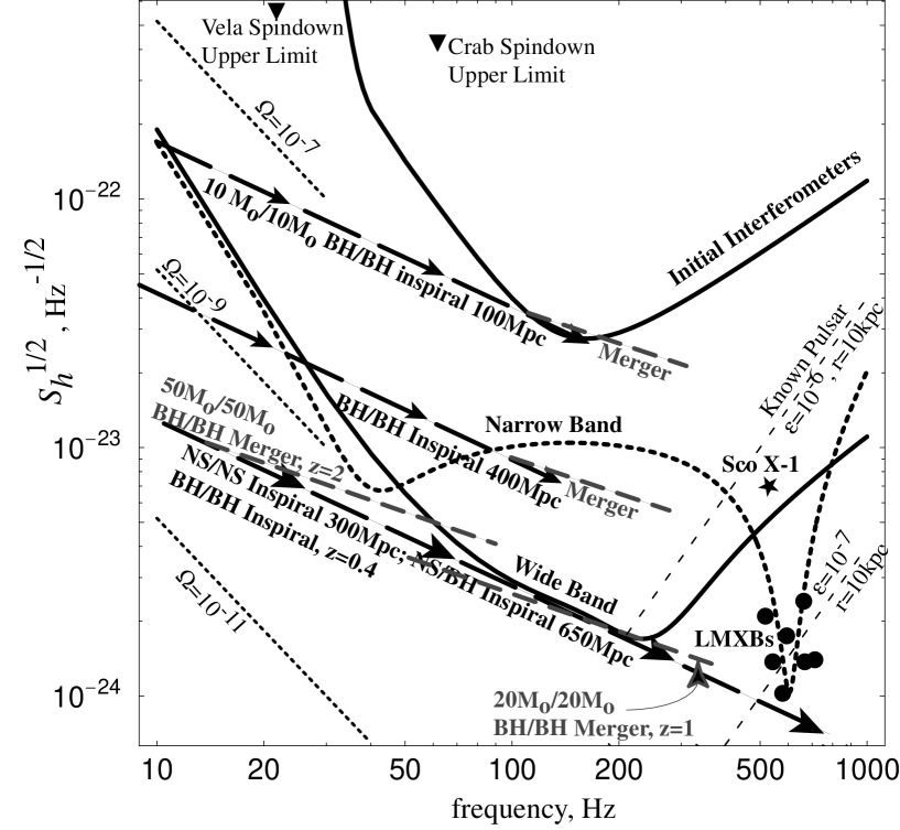
Figure 6: Comparison of source strength to noise magnitude for several astrophysical gravitational-wave sources. The heavy black bands are the various incarnations of LIGO interferometers: initial (top, solid), advanced in wide band configuration (bottom, solid), advanced in narrow band configuration (bottom, dotted). The meaning of the various source markers included here is described in the text. (Figure adapted by Kip Thorne for our use, from Ref. ligo_mature .)

Figure 6 illustrates several important gravitational-wave sources compared with LIGO noise curves. The noise curves shown are the amplitude spectrum ${\tilde{h}}$, with units ${\rm Hz}^{-1/2}$, for first generatation detectors, and for advanced detectors in both wide and narrow band configurations explain_sensitivity . For each source, the plotted strain ${\tilde{h}}_{s}$ is defined such that the ratio is equal to the ratio of signal strength $S$ to noise threshold $T$, rms averaged over all source directions and orientations: ${\tilde{h}}_{s}/{\tilde{h}}=\langle S^{2}/T^{2}\rangle^{1/2}$. The threshold is set assuming that the best practical data analysis techniques have been applied, and that the probability of a false alarm is one percent. Thus, a source that touches the noise in this figure is at the threshold for detection. Details of how the threshold is computed for each source are discussed in the following subsections.

III.2.1 Compact binaries

Coalescing compact binary star systems are currently the best understood sources of gravitational waves. Members of such binaries are compact, collapsed stellar remnants — neutron stars or black holes. Double neutron star binaries are observed in our galaxy; detailed studies of these systems hulse_taylor ; taylor_weisberg ; stairsetal provide what is currently our best data on gravitational-wave emission and led to Joseph Taylor and Russell Hulse winning the Nobel Prize in 1993. The galactic binary neutron star systems have orbital periods of several hours, radiating at $\mbox{several}\times 10^{-4}\,{\rm Hz}$, far beyond the range of ground-based detectors. Gravitational waves carry energy and angular momentum away from the system, driving the neutron stars to inspiral towards one another. The emitted waves sweep upwards in frequency and amplitude as the neutron stars come closer together. In several hundred million years, the gravitational waves from a galactic binary will enter the frequency band of LIGO detectors; about 10 minutes later, their neutron stars will violently collide and merge into a single object.

A few hundred million years is a bit long to run an experiment, so gravitational-wave detectors must be sensitive to a large volume of the universe in order to obtain an interesting event rate. Extrapolating from the observed population to the universe at large (see, e.g., Refs. nps ; phinney91 ; kalogera_lorimer ) suggests that in order to measure an interesting rate of events (several per year), detectors must be sensitive to coalescences hundreds of megaparsecs away. Extrapolation can only predict the rate of binary neutron star systems, since those are the only compact binaries that have been observed to date. Another method is population synthesis: modeling stellar evolution to predict the rate of compact binary formation from a population of main sequence stars (see, e.g., Refs. bethebrown ; fwh ; belczynbulik ; pzy ; pzm ). Population synthesis predictions span a rather wide range — not surprising, since much of the underlying physics is rather uncertain. Most calculations agree at least to within an order of magnitude with the extrapolated predictions for binary neutron star coalescence. This is by design: the calculations are “tuned” to match the data for binary neutron stars. Predictions for other compact binary systems, neutron star-black hole and black hole-black hole, vary quite a bit bethebrown ; pzy ; pzm . Good data from gravitational-wave detectors will have a large impact on our understanding of stellar evolution and compact binary formation.

The entire coalescence process can be usefully (albeit somewhat crudely) divided into three broad epochs flanhughes : the inspiral, in which the binary’s members are widely separated and spiral inward due to gravitational-wave backreaction; the merger, in which the binary’s orbit becomes dynamically unstable, and the two bodies merge into a single object; and (possibly) the ringdown, in which the merged remnant settles down to a stationary, rotating (Kerr) black hole. The ringdown only occurs if the binary leaves a black hole behind after coalescence. This broad characterization is rather oversimplified, but useful, providing a qualitative description of the system’s dynamics and wave emission. Further discussion of these epochs in the context of current research on coalescing binaries is given in Sec. V.

Dividing the system’s evolution into three epochs likewise divides the gravitational-wave signal into three broad frequency bands. This is one reason that this crude characterization is useful: it gives some sense of what source dynamics are accessible to the observatories. Consider first the inspiral. Very roughly speaking (cf. discussion in Sec. IIIB of Ref. flanhughes ),

$$\mbox{inspiral waves:}\qquad f\lesssim 400\,{\rm Hz}\left[10\,M_{\odot}\over(1+z)M\right]\;.$$ (8)

(Here, $z$ is the cosmological redshift.) Likewise, we can with a fair degree of confidence characterize the frequency band of the ringdown waves. Using black hole perturbation theory teuk73 ; leaver , we find that the mode that is most likely to dominate after binary coalescence has

$$\mbox{ringdown waves:}\qquad f \sim {c^{3}\over 2\pi G(1+z)M}\left[1+0.63(1-a/M)^{0.3}\right]$$ (9)

$$\sim (1200-3200)\,{\rm Hz}\left[10\,M_{\odot}\over(1+z)M\right]\;.$$

The Kerr spin parameter $a$ varies from 0 to $M$; the span in frequency reflects this range. Merger waves are then all waves emitted at frequencies between these two extremes.

Note that all frequencies scale inversely with the redshifted mass, $(1+z)M$. The redshift factor should be fairly obvious, since $1+z$ is precisely the factor by which radiation’s wavelength changes due to cosmological evolution. The inverse mass dependence enters because the mass sets all timescales relevant to the radiation. Since frequency is an inverse timescale, all frequencies are proportional to inverse mass.

As mentioned in the discussion of the LDAS architecture, some systems will be analyzed using matched filtering, correlating the experimental data with theoretical waveform models, known as templates cutflan ; ben . Matching a template to the signal boosts the signal-to-noise ratio (SNR) by a factor that is roughly $\sqrt{N}$, where $N$ is the number of measured gravitational-wave cycles. Because the ringdown and early inspiral are rather well-understood, we are confident in our templates for those coalescence epochs; the late inspiral and merger epochs are rather more poorly understood. This motivates much research in relativity theory today.

The tracks illustrating compact body coalescence in Fig. 6 assume that matched filtering is applied. The thresholds are computed assuming that matched filters are used to integrate the signal at each frequency over bands of width $\Delta f\sim f$. We assume that data from all three LIGO interferometers is combined. For neutron star-neutron star binaries, only the inspiral waves are easily accessible to ground-based detectors. As will be mentioned in Sec. V.3, narrow banded interferometers and acoustic detectors will be able to provide some information about the high frequency binary neutron star merger signal. The binary neutron star signal is fairly weak; for assured detection by first detectors (amplitude SNR $\sim 5$ in all LIGO interferometers), the binary can be no further than about 20 Mpc. We must go much farther out to obtain an interesting rate of neutron star coalescences. As a consequence, current wisdom is that neutron star-neutron star detection by first detectors, though plausible, is not likely. However, detection after upgrade is quite likely — by Figure 6, neutron star-neutron star coalescence should be seen out to about 300 Mpc. Non-detection of binary neutron star coalescence by advanced interferometers would be rather surprising.

Neutron star-neutron star waves are weak because of the system’s relatively small mass. Increasing the mass increases the signal, but shifts all frequency bands downward. The shift in frequency causes much of the inspiral to shift out of band, leaving the very late stage of inspiral and the merger in LIGO’s most sensitive band. Figure 6 shows that for the more massive binary black hole systems, the late inspiral and merger waves are likely to be the most relevant for detection. The fact that these rather poorly understood epochs of binary black hole coalescence are right in the most sensitive band of ground-based detectors greatly motivates theoretical work to understand this waves better. If we succeed in modeling the late inspiral and merger accurately, these signals should be detectable at cosmological distances, with redshift $z\sim 0.5-1$.

III.2.2 Stochastic backgrounds

Stochastic backgrounds are “random” gravitational waves, arising from a large number of independent, uncorrelated sources that are not individually resolvable. A particularly interesting source of backgrounds is the dynamics of the early universe — an all sky gravitational-wave background, similar to the cosmic microwave background. Backgrounds can arise from amplification of primordial fluctuations in the universe’s geometry, phase transitions as previously unified interactions separated, or the condensation of a brane from a higher dimensional space. Mechanisms of this kind and their connections to unification physics are discussed in Sec. V.4; here, we briefly discuss how these backgrounds are characterized and the levels of sensitivity LIGO should achieve.

Stochastic backgrounds are always discussed in terms of their contribution to the universe’s energy density, $\rho_{\rm gw}$. In particular, one is interested in the energy density as a fraction of the density needed to close the universe, over some frequency band:

$$\Omega_{\rm gw}(f)={1\over\rho_{\rm crit}}{d\rho_{\rm gw}\over d\ln f}\;.$$ (10)

Different cosmological sources produce different levels of $\Omega_{\rm gw}(f)$, centered in different bands. Amplified primordial fluctuations surely exist, but are likely to be rather weak: estimates suggest that the spectrum will be flat across LIGO’s band, with magnitude $\Omega_{\rm gw}\sim 10^{-15}$ turner . Waves from phase transitions can be significantly stronger, but are typically peaked around a frequency that depends on the temperature $T$ of the phase transition:

$$f_{\rm peak}\sim 100\,{\rm Hz}\left({T\over 10^{5}\,{\rm TeV}}\right)\;.$$ (11)

We note here that the temperatures required to enter the LISA band, $f\sim 10^{-4}-10^{-2}$ Hz, is $T\sim 100-1000\,{\rm GeV}$, nicely corresponding to the electroweak phase transition. Waves arising from extradimensional dynamics should peak at a frequency given by the scale $b$ of the extra dimensions hogan_prl ; hogan_prd :

$$f_{\rm peak}\sim 10^{-4}\,{\rm Hz}\left({1\,{\rm mm}\over b}\right)^{1/2}\;.$$ (12)

For the waves to be in LIGO’s band, the extra dimensions must be rather small, $b\sim 10^{-15}$ meters. LISA’s band is accessible for a scale similar to those discussed in modern brane-world work randallsundrum1 ; randallsundrum2 .

The detectable magnitude of $\Omega_{\rm gw}(f)$ and the sensitive frequency band depend on the particular instrument. LIGO will measure stochastic backgrounds by comparing data at the two sites and looking for correlated “noise” maggiore ; allen_romano . For comparing to a detector’s noise, one should construct the characteristic stochastic wave strain,

$$h_{c}\propto f^{-3/2}\sqrt{\Omega_{\rm gw}(f)\Delta f}\;.$$ (13)

(For further discussion and the proportionality constants, see maggiore .) Stochastic backgrounds are illustrated in Fig. 6 as the downward sloping dotted lines, labeled $\Omega=10^{-5}$, $\Omega=10^{-7}$, etc. These curves assume $\Delta f\sim f$. Early detectors will have fairly poor sensitivity, sensitive to a background at levels $\Omega_{\rm gw}\sim 5\times 10^{-6}$ in a band from about 100 Hz to 1000 Hz. This is barely more sensitive than known limits from cosmic nucleosynthesis allen_review . Later upgrades will be significantly more sensitive, able to detect waves with $\Omega_{\rm gw}\sim 10^{-10}$, which is good enough to place interesting limits on cosmological backgrounds.

III.2.3 Stellar core collapse

Another promising source of radiation for ground-based detectors is the core collapse of massive stars. When massive stars die their most dense central regions catastrophically collapse, driving the star to explode in a supernova and the innermost matter concentrations to form a neutron star or black hole. The conditions for strong gravitational wave emission — highly energetic dense matter dynamics — are clearly met. However, because stellar collapse is not very well understood, our understanding of gravitational-wave emission from such collapse is rather uncertain.

One of the major goals of gravitational-wave observatories is to coordinate gravitational-wave detection with external observations. This will be particularly important for stellar core collapse due to our poor understanding of the likely gravitational waves emitted in that case — coincident detection with neutrino, gamma ray, and/or optical observatories will greatly increase confidence in the measurements, as the combined network of instruments provides triggers and cross-checks for each other. Coincident detection and measurement will produce great science payoff aside from increased confidence and cross-checks. For example, a supernova in our galaxy would be easily detected by both neutrino and gravitational-wave observatories. Measurement of such events will paint a far more solid picture of collapse dynamics than our current view, tracking the relative evolution of processes that generate neutrinos with the dense matter dynamics. An event in our galaxy would have very large SNR, so such studies could be done with high precision. Such nearby events will be very rare (the supernova rate is estimated to be several events per galaxy per century), but would provide enormous scientific payoff.

A review of gravitational waves from stellar collapse, focusing on their relevance to gravitational-wave observatories, has recently appeared fhh ; our discussion is largely based on that paper. The strongest core collapse gravitational waves come from instabilities that can develop in the matter dynamics. One of the most-discussed instabilities is bar formation: the tendency of rotating matter to go into a non-axisymmetric, rotating, bar-shaped mode. A bar mode is potentially a strong source of radiation. Many numerical simulations tohline85 ; durisen86 ; williams88 ; houser94 ; smith96 ; houser96 ; pickett96 ; houser98 ; new00 have shown that bar modes are promising sources, though usually with rather simplified models. Ref. fhh looked at the potential for bar mode instability in a variety of realistic stellar collapse scenarios, and found that it still remains a promising source of waves for ground-based observatories, though much work remains to be done to clarify the waves’ characteristics in different circumstances. For example, bar modes will only be unstable if the precollapse progenitor is rotating sufficiently rapidly. This appears likely for many supernova progenitors. It may also be the case in “accretion induced collapse” (AIC) of some white dwarf stars, though the conditions for this to occur and its likely rate make AIC much less promising as a source lindblomliu ; liu ; liu_private .

In some star collapses, the distribution of density and angular momentum is such that the dense inner material may fragment into pieces, forming “chunks” that rapidly orbit for some time before settling into an equilibrium. These orbiting chunks would be copious gravitational-wave radiators. Van Putten has recently argued that such a matter distribution is likely to form in the progenitor to a gamma-ray burst (cf. Ref. mhvp and references therein). Gamma-ray bursts may thus be accompanied by an extraordinarily strong burst of gravitational radiation. Fryer, Holz, and Hughes fhh find that a fragmentation instability may allow ground-based detectors to observe the collapse of population III stars — a putative population of extremely massive ($\sim 100-300\,M_{\odot}$) stars that formed and died early in the universe’s history. This is an example of new astrophysics that gravitational-wave astronomy may discover.

III.2.4 Periodic sources

Periodic sources of gravitational waves are emitters which radiate at constant frequency (or nearly constant frequency), much like radio pulsars. At first sight, this suggests they might be easy to detect — it should be simple to coherently follow a periodic source’s phase evolution, allowing us to build up enough power for an intrinsically weak signal to stand above noise. However, the signal is strongly modulated by the earth’s rotation and orbital motion, “smearing” the wave across multiple frequency bands and greatly degrading the source’s strength. Searching for periodic gravitational waves means demodulating the motion of the detector. This is computationally arduous — the modulation is different for every sky position. Unless one knows in advance the position of the source, one needs to search over a huge number of sky position “error boxes”, perhaps as many as $10^{14}$. One rapidly becomes computationally limited. For further discussion, see periodic ; for ideas about doing hierarchical searches, requiring less computational horsepower, see per_hierarchical .

The prototypical source of continuous gravitational waves is a rotating neutron star. If the neutron star is non-axisymmetric (for example, it has a crust that is somewhat oblate and misaligned with the star’s spin axis), it will radiate gravitational waves with characteristic amplitude

$$h_{c}\sim{G\over c^{4}}{If^{2}\epsilon\over r}\;,$$ (14)

where $I$ is the star’s moment of inertia, $\epsilon$ characterizes the degree of distortion (see periodic and references therein for further discussion), $f$ is the wave frequency, and $r$ is the distance to the source. Realistic choices for these parameters suggest that $h_{c}\sim 10^{-24}$ or smaller. To measure these waves, we need to coherently track the signal for a large number of wave cycles. Coherently tracking $N$ cycles boosts the signal strength by a factor $\sim\sqrt{N}$.

The characteristic amplitude of several possible pulsars are illustrated in Fig. 6. The points labeled “Crab” and “Vela” illustrate the maximum possible gravitational-wave strength that the well-known Crab and Vela pulsars could emit. This pulsars are known to “spin down”; that is, their rotation periods are observed to decrease over time. Figure 6 assumes that all of this spindown is due to gravitational-wave backreaction, an assumption that is known to be wrong. The waves from these pulsars will be much weaker; however, since their sky position and frequencies are known in advance, it will not be too difficult to search for any waves they might emit. The upward sloping lines labeled “Known pulsar, $\epsilon=10^{-6},10^{-7}$, $r=10\,{\rm Kpc}$” illustrate the waves produced by a source whose position is known but frequency is unknown, if the distance and deformation are as indicated. In all of these cases, it is assumed that the signal can be coherently tracked for several months, building up power.

A nearly periodic source of gravitational waves from rotating neutron stars is the r-mode instability, a fluid instability that may be active in hot, fluid neutron stars andersson ; friedman_morsink ; lom ; aks . This mode is not perfectly periodic, since radiative backreaction rapidly reduces the star’s spin and gravitational-wave frequency; but it is nearly so, and search techniques for r-mode active stars are likely to be very similar to searches for periodic sources olcsva .

Finally, we note that neutron stars accreting matter from a close companion may be periodic sources of gravitational radiation lars ; ubc . This would explain why most neutron stars in such low mass x-ray binary (LMXB) systems appear to have a maximum spin frequency: rather than spinning up indefinitely by the matter accreting onto them, they eventually are braked by gravitational-wave backreaction. Such sources are very promising targets for observation since their sky positions are known very accurately from x-ray observation. Since they are in binaries, though, their waveforms will be even more strongly modulated than “normal” radiating pulsars. The points on Fig. 6 labeled “Sco X-1” and “LMXBs” show waves that are possible from known LMXB systems. Many of these systems will only be detectable in the narrow-banded configuration, demonstrating the science impact possible with tunable interferometer configurations.

IV Space-based detectors

Many promising sources of gravitational waves radiate at low frequencies, from a few microHz to about a Hz, where Earth-based detectors have very poor sensitivity due to geophysical noise. Such sources include massive black hole systems, compact binaries, very close normal binaries, and cosmological backgrounds. To get away from the geophysical background, the detector must be located in space. In this section, we describe the space-based detector LISA which will target these low-frequency sources. We first describe the LISA mission, and then discuss certain sources that are of particular interest for LISA science. More extensive information on the mission and additional references are given in Refs. prephaseA ; intlisa_1 ; intlisa_2 ; bender .

IV.1 Description of the LISA Mission

The Laser Interferometer Space Antenna (LISA) is designed to detect and study in detail gravitational-wave signals at frequencies from roughly 10 microHz to 1 Hz. Once the conclusion to build a low-frequency, space-based detector has been reached, it becomes attractive to make the size of the antenna quite large. Using laser heterodyne measurements between widely separated spacecraft, even with 1 W power levels, antenna sizes of millions of kilometers are feasible. The measurements are made between freely floating proof masses, inside the spacecraft, that are very carefully shielded from both internal and external disturbances. With this approach, very desirable sensitivity levels can be achieved throughout the planned frequency range.

The LISA mission is planned as a joint mission of the European Space Agency and NASA, for launch in about 2010. The antenna will be based on laser measurements between three spacecraft located at the corners of an equilateral triangle that is 5 million km on a side. A one year orbit around the Sun for each spacecraft has been found such that: (a) the spacecraft separation stays constant to better than $1\%$ over more than 10 years; (b) the center of the antenna is on a circular orbit in the ecliptic plane and about 50 million km ($20^{\circ}$) behind the Earth; (c) the plane of the antenna is tipped at $60^{\circ}$ to the ecliptic, and that plane rotates around the pole of the ecliptic with a one year period; and (d) the antenna rotates within that plane with a one year period. The orbits each have an eccentricity of about 0.01, and an inclination that is the square root of 3 times the eccentricity.

The main components of the payload for each spacecraft are located within a Y-shaped thermal shield made of carbon fiber reinforced plastic, which has a low coefficient of thermal expansion. There are two cylindrical optical assemblies about 1 m long and 0.35 m in diameter that point out along two of the arms of the Y and toward the distant spacecraft. A schematic drawing of one optical assembly is shown in Fig. 7. Only a brief description of its operation will be given here.

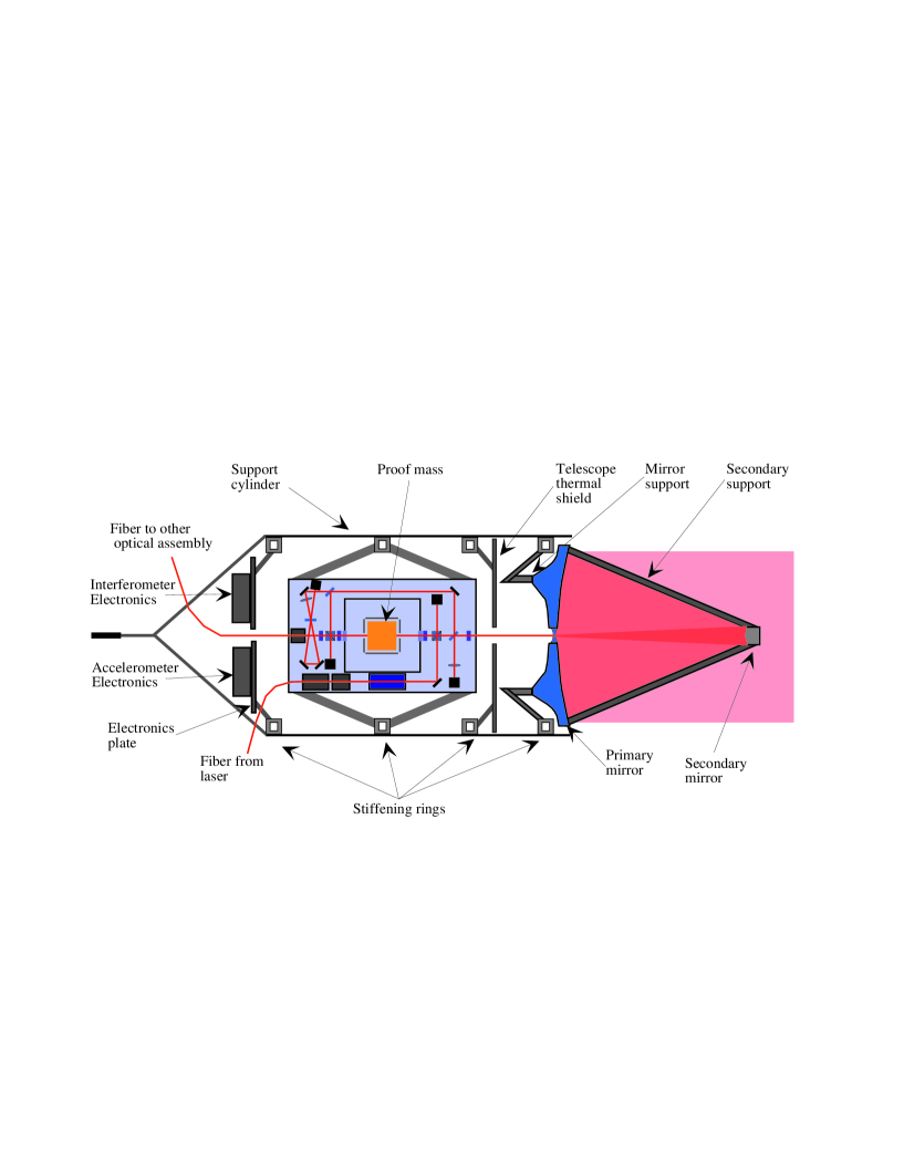
Figure 7: Schematic of the LISA optical assembly.

The rectangular structure located near the center of the optical assembly is the optical bench. It is supported by a Wheatstone bridge mounting from the optical assembly support cylinder so that temperature gradients along that cylinder don’t get transmitted conductively to the optical bench. The gravitational sensor is mounted at the center of the optical bench, and contains the freely floating proof mass and the housing around it. Capacitive bridge measurements between a number of pairs of capacitive plates on the inside of the housing and the proof mass determine even small translations and rotations of the proof mass with respect to the housing. The laser measurements of changes in the distances between the proof masses in different spacecraft are made to the front face of each proof mass through a small window in the outer enclosure of the gravitational sensor.

Light from the 1.06 micron Nd:YAG laser (not shown) is brought onto the optical bench through a fiber, and almost all of it is sent by a polarizing beamsplitter to the 0.3 m diameter transmit/receive telescope. The transmitted beam has a diameter of about 20 km when it reaches the distant spacecraft, and a small portion of it is collected by the telescope there. This light goes through the beamsplitter, is reflected from the face of the proof mass, and is then deflected by the beamsplitter to go to a photodiode detector. Some light from the on-board laser also goes to the photodiode, and the beat between the received beam and this local laser beam is one of the six main signals generated by the antenna. Each beam propagating in one of the two directions along one of the three sides of the antenna is used in generating one of the six main signals.

Because of the choice of spacecraft orbits, the lengths of the sides of the triangle stay constant in length to better than $1\%$ over 10 years or longer, even including planetary perturbations. However, the resulting relative velocities are still on the order of 10 m/s, and cause Doppler shifts of up to roughly 10 MHz at some times. These Doppler shifts vary typically with periods of several months or longer and in an extremely smooth fashion, so that they can be fitted out from the observations. The gravitational waves will cause phase variations in the LISA signals that can be analyzed after the huge but much lower frequency Doppler shifts have been fitted out.

To understand how the LISA antenna works, it is useful to consider only two sides of the triangle, with the spacecraft common to both sides being the master spacecraft. The lasers at the two distant spacecraft are assumed to be phase locked to the received laser beams, so that the return beams have the same phase as if the beams were just reflected by mirrors. Thus the system acts like a Michelson interferometer, but with two signals generated back at the master spacecraft that give the variations in the length of each of the interferometer arms separately. To the extent that the proof masses at the ends of the arms really are undisturbed by spurious accelerations, the apparent variations in the sum of the lengths of the two arms will almost all be due to phase noise in the laser. This information then can be used to correct the difference in length of the two arms in software for the laser phase noise, which otherwise would swamp the gravitational wave signals.

An Industrial Phase A Study of the LISA mission was carried out for the European Space Agency and presented to their scientific community in September 2000. The spacecraft, payload and mission designs from this study, which started from the results of earlier studies in both Europe and the US, essentially form the current baseline plan for the mission. Under this plan, each spacecraft is 2.7 m across and 0.56 m high, with the sides slanted in at $30^{\circ}$ so that sunlight only hits the top surface, where the solar cells to provide power are mounted. The optical assemblies point out through the slanted sides, and the direction to the Sun makes a constant $30^{\circ}$ angle with respect to the top of the spacecraft. This keeps the temperature and temperature distribution in the spacecraft extremely constant. This is a major reason why the time variations in spurious forces acting on the carefully shielded proof masses deep in the spacecraft can be kept extremely low.

Each spacecraft initially has a propulsion module attached to it, and the three combined units are stacked up and launched by a single launch vehicle into roughly 13 month period elliptical orbits around the Sun. After leaving the Earth, the units separate and their propulsion units carry them to their desired orbits over a period of roughly a year. The orbits are checked for a few weeks by tracking with NASA’s Deep Space Network, and minor orbit corrections are made as needed. The propulsion modules then separate gently from the spacecraft and drift away. After separation, the spacecraft are oriented properly with their optical assemblies pointing at the other spacecraft forming the antenna. This is done using continuously operating and electrically controllable micronewton thrusters mounted on the spacecraft.

Next, the proof masses are released from the clamping mechanisms that have held them during launch and electrical forces are applied to move them to the centers of their housings. Then, the control laws for the micronewton thrusters are changed so that they also take on the job of making the spacecraft follow the average position of the two proof masses. The motion of the spacecraft is then determined by the forces acting on the proof masses, and the effect of non-gravitational forces on the spacecraft can be essentially eliminated. This is called a drag-free system, since such systems were first used to greatly reduce the drag on Earth satellites due to the residual atmosphere. For LISA, since there are two proof masses, weak electrical forces perpendicular to the laser beam directions are still applied to the proof masses to keep them centered in their housings.

The capacitive position measurements are sensitive enough and the noise in the thrusters low enough that the relative motion of the spacecraft with respect to the proof masses can be kept very low. This is another reason why the variations in spurious forces on the proof masses can be kept very low. The total thrust needed is mainly the roughly 20 micronewtons required to buck out the solar radiation pressure, and varies only slightly.

Finally, a beam acquisition procedure is started to successively turn on each laser and adjust its pointing direction accurately. When all six main signals are obtained, the scientific part of the mission can begin. The nominal scientific mission lifetime may be as short as two or three years, but it is hoped that the observations can continue for about a decade. The thrust required from the micronewton thrusters is low enough that the reaction mass needed even for a decade of operation is small.

IV.2 LISA Sensitivity and Galactic Binaries

The instrumental sensitivity of the LISA antenna is determined by two factors. One is the noise in measuring changes in the distances between the different proof masses. The second is the level of spurious accelerations of the proof masses. From noise budgets for these two different types of noise, a threshold sensitivity curve for LISA can be determined. Such a curve is shown in Fig. 8, along with some information about expected signals from binary stars in our galaxy that will be discussed later. The sensitivity curve shown is for 1 year of observations and an amplitude SNR of 5.

Nearly all of the resolvable galactic binary sources expected for LISA will be thousands to millions of years from coalescence, and thus their frequencies will change little over a few years. Each can be represented by a single point giving the rms gravitational-wave amplitude and frequency (twice the orbital frequency). If that point lies above the sensitivity curve, then there is enough signal to overcome the instrumental noise with 1 year of observations and a SNR of 5. This SNR is needed to be confident of detection for a source whose sky position and frequency are not known.

There is of course an error allocation budget for each of the two types of noise. In such a budget, allowable levels of error are assigned to each of the expected or possible sources of error in the measurements. For measuring changes in the distances between proof masses, the total error budget level for the round-trip arm length difference of two antenna arms is 40 picometers per root Hz (pm/rtHz), independent of frequency (white noise) down to below 1 millihertz (1 mHz). This is called the spectral amplitude of the noise, and is defined as the square root of the power spectral density. The noise power in a narrow bandwidth is proportional to the bandwidth, with units of [(pm)²]/Hz, so the spectral amplitude has units of pm/rtHz.

Most of the expected distance measurement noise comes from shot noise in the detected laser photons. The rate of photon detections for the received signal is a few times $10^{8}$ per second, so measurements can be made to roughly $1/(2\pi\sqrt{10^{8}})\sim 10^{-5}$ of a laser wavelength in 1 second, or about $10^{-21}$ in 1 second for the fractional change in the round-trip distance. There is some additional contribution to the error due to jitter in the pointing of the laser beam toward the distant target and other noise sources, but they are relatively small.

The LISA sensitivity curve at frequencies substantially above 3 mHz is determined by the distance measurement noise. At lower frequencies, the instrumental sensitivity is limited mainly by spurious accelerations of the proof masses. There are roughly half a dozen sources of such acceleration noise that dominate the error budget, and they are assigned equal error levels. With allowances for other smaller acceleration noise sources, the rms total is $3\times 10^{-15}$ meters sec^-2/rtHz down to 0.1 mHz, and somewhat higher at still lower frequencies. A space validation flight for the subsystem consisting of the proof mass, its housing, and the associated electronics currently is planned in order to verify that they perform according to their design specifications.

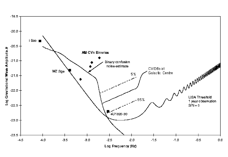
Figure 8: LISA sensitivity curve, with a few interesting sources. Points are the expected signal amplitude of certain already known monochromatic binary stars; “CWDB” stands for close white dwarf binary.

With the sensitivity curve shown in Fig. 8, LISA will be able to observe signals from many binaries in our galaxy. In order for the two members of a binary to be close enough together to have gravitational wave frequencies above about 0.1 mHz, both must be compact objects — white dwarf stars, neutron stars, or black holes. The number of such binaries in our galaxy is roughly $10^{8}$; most will be close white dwarf binaries. Below 1 or 2 mHz there will be more than one in each 1 cycle/year frequency resolution bin, so that individual ones cannot be resolved. The curve labeled “confusion noise estimate” in Fig. 8 represents the expected noise level due to the random superposition of such signals.

At higher frequencies, the number per bin drops rapidly with increasing frequency, as they lose energy more and more rapidly by gravitational-wave emission. About 3000 will be resolvable above about 3 mHz. Roughly $90\%$ of them will have amplitudes between the curves labeled $5\%$ and $95\%$ in the figure. The direction and frequency of only a few of them will be known ahead of time, and some of these are shown.

IV.3 Massive Black Hole Binaries

There are at least three types of events involving massive black holes (MBHs) that appear likely to produce signals observable by LISA. However, the event rates can only be estimated very crudely, and this situation seems unlikely to change much in the near future. The primary objective of the LISA mission is to detect such signals and study them in detail. But none of these signals are guaranteed to be present, so the present design of the LISA antenna has been chosen to make as many of the types of MBH signals observable as possible.

The first type of signal of strong interest is associated with the origin of massive black holes. An important question is how the seed MBHs that later grew to be the massive and supermassive black holes observed today were formed. We label black holes with masses $M\sim 1.5-100\,M_{\odot}$ “stellar mass black holes” (potentially formed by the evolution of massive stars); holes with mass up to about $3\times 10^{7}\,M_{\odot}$ are labeled “massive black holes” (MBHs); and still larger ones “supermassive black holes”.

There are several theories for how seed MBHs form. In one, stellar mass black holes sink to the center in a dense galactic core by dynamical friction, and collisions lead to the formation of higher mass objects. The largest black hole grows faster than all others, swallowing up holes comparable size. This becomes the seed for growth of an MBH of perhaps $10^{5}\,M_{\odot}$ or larger. When it reaches a mass of roughly $10^{3}\,M_{\odot}$, it would be able to continue growing fairly rapidly by absorption of gas in the galactic nucleus and by tidal disruption of stars quinshap .

An alternate scenario postulates a dense cloud of gas and dust, evolving to the point where it becomes optically thick. Radiation pressure plus magnetic fields then prevents further fragmentation of the cloud to form stars haehnelt_rees . At that point, if energy and angular momentum can be dissipated fairly rapidly, several things might happen. One possibility is that a supermassive “star” with mass $M\sim 10^{5}-10^{6}\,M_{\odot}$ forms. This would be subject to a pulsational instability mtw that drives it to collapse into a MBH. Another possibility is that the cloud may become dense enough to reach the point of relativistic instability and collapse directly to a MBH without going through the supermassive star stage.

From the standpoint of LISA observations, the major issue of the collisional growth scenario is whether some of the individual black holes become large enough before merging with the largest hole that their coalescence is detectable. An example mass pair that would just be detectable during the last year before coalescence at $z=1$ $m_{1}=m_{2}=300\,M_{\odot}$; another is $m_{1}=50\,M_{\odot}$, $m_{2}=3000\,M_{\odot}$. The lowest straight curve in Fig. 9 shows the signal strength and frequency evolution during the year before coalescence of a binary with $m_{1}=m_{2}=500\,M_{\odot}$ at $z=1$. The ticks along this line represent times 0.0, 0.2, 0.4, 0.6, 0.8, and 0.99 year from the beginning of the last year. Such a signal would be observable even from a coalescence at $z=5$. The other curves in the figure will be discussed later.

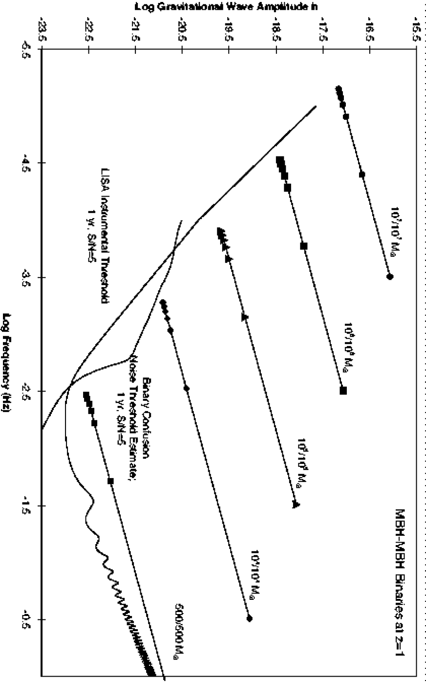
Figure 9: LISA sensitivity curve compared to the wave amplitude for binary black hole mergers.

A second important signal comes from black holes of roughly $10\,M_{\odot}$, neutron stars, or white dwarfs in orbit around MBHs in galactic nuclei. Such highly unequal mass systems will result from compact objects in the cusp around the MBH being scattered in close enough to start losing energy by gravitational radiation, becoming progressively more tightly bound. The orbits remain elliptical throughout in this case, and during the last year the orbital speed near periapsis can reach almost half the speed of light. The period for periapsis precession is similar to that for radial motion; rapid frame-dragging may also be present. Thus the orbits are extremely non-Newtonian, as discussed later. From the astrophysics point of view, the number and type of systems of this kind observed will give valuable information about a combination of the distribution of MBH masses in galactic nuclei and the space density of compact objects in the cusps around MBHs.

The third and strongest type of MBH signal expected for LISA is from the coalescence of binaries consisting of two MBHs, where both are substantially more massive than $10^{3}M_{\odot}$. Such events can follow the mergers of galaxies or pre-galactic structures, provided that two conditions are fulfilled. First, the pre-merger structures must already contain MBHs; second, the MBHs must form a close binary in substantially less than the age of the universe. Present estimates are that these conditions have been fulfilled frequently enough to give one or more MBH coalescences per year, but even this is uncertain. It seems likely that coalescences involving MBHs of roughly $10^{5}-10^{6}M_{\odot}$ will be the most common; mergers of structures with $10^{7}\,M_{\odot}$ or more massive MBHs may well be less frequent, and less massive MBHs may have difficulty forming close binaries.

The signal strength during the last year for equal-mass MBH coalescences at $z=1$ are shown in Fig. 9. Since the SNR ratios are high, such events would be easily observable anywhere in the universe. The waves from these events will be measured sufficiently well that detailed parameter fits will be possible untangling , making possible much astrophysical analysis. However, since the event rate is definitely not guaranteed, efforts will be made to keep the acceleration noise level at frequencies below 0.1 mHz as low as possible. This will increase the chances of seeing coalescences or $10^{5}$ or $10^{6}\,M_{\odot}$ MBHs a number of years before coalescence, and thus improve the statistical information on them.

IV.4 LISA and stochastic backgrounds

By their very nature, stochastic gravitational waves are difficult to distinguish from noise. As described in Sec. III.2.2, ground-based detectors can find them by coordinated measurements, essentially comparing the outputs of multiple detectors to find sources of correlated noise. Provided there are no common noise sources (which, due to their wide separation, should be the case), this should work well.

LISA is a single space-based antenna and so cannot use this technique, but has other tools that can be employed instead. In particular, it is possible to combine the signals from LISA’s spacecraft in such a way that the detector is insensitive to gravitational waves armstrongetal . Observables of this kind are called “Sagnac” observables, since they correspond to observables constructed from phase information that propagates around the LISA antenna, as in a Sagnac interferometer. Since the Sagnac observable is insensitive to gravitational waves, it measures noise alone. In this way, one can detangle the noise-like signature of a stochastic background from the actual interferometer noise hoganbender . LISA’s stochastic background sensitivity should then be limited by the Galactic white dwarf background (a somewhat prosaic stochastic background). This will allow it to set strong limits on cosmological backgrounds in its band, corresponding to an energy density about a million times smaller than the cosmic microwave background.

LISA’s band is fortuitously placed to measure potentially interesting cosmological sources, as has been mentioned already in Sec. III.2.2. An electroweak phase transition, occuring when the temperature of the universe was $T\sim 100-1000$ GeV, generates waves peaked at a frequency $f\sim 10^{-4}-10^{-3}$ Hz. Such waves could be directly detected by LISA apredaetal . Likewise, waves from extradimensional dynamics are likely to be in LISA’s band for extra dimensions on the scale of millimeters to microns hogan_prl ; hogan_prd . As discussed in the next section, LISA is well situated to at least put stringent limits on many early universe scenarios, and perhaps directly detect stochastic waves.

V New tests of physics and tests of new physics

As should be clear from the discussion of sources given in Secs. III and IV, the routine detection of gravitational waves will certainly transform the field of astronomy. The rarest and most obscure cosmic events, such as black hole mergers, will suddenly achieve a phenomenological prominence appropriate to their huge power output. Populations barely detected at all today, such as white dwarf binaries, will produce a din that overwhelms even the LISA instrumental noise sources. The current orders-of-magnitude uncertainties in rates and intensities of all kinds of gravitational-wave sources clearly indicates our ignorance of the dominant mass-energy flows. We will learn about details of many things that astrophysicists regard as fundamental: the dynamics of massive black hole formation in the centers of galaxies, the evolution of binary star systems, perhaps the equation of state of nuclear matter and the mechanism of neutrino-driven supernova explosions.

Readers of these proceedings will be more interested in new physics than new astrophysics. These observatories should not be regarded as “merely” tools of astronomers; they will probe phenomena that will either constrain or reveal something new about the laws of nature. We discuss these possibilities in the subsections below. We first describe how gravitational-wave observatories will probe the nature of extremely strong gravity. Section V.1 discusses the gravitational-wave probes of highly dynamic gravity that will be studied in the merger of binary black hole systems; Sec. V.2 focuses on measurements that will map in detail the structure of black hole spacetimes. It is worth noting at this point that it is still not conclusively known whether the massive objects usually described as “black holes” in fact are black holes as described by Einstein gravity (though the evidence from sources such as x-ray telescopes is getting better and more conclusive all the time). Section V.3 discusses how tracking gravitational waves from systems with neutron stars may be used to study the properties of dense nuclear matter, probing its equation of state. Finally, in Sec. V.4 we examine what kinds of “new physics” may be probed, focusing in particular on how gravitational waves may be used to test new ideas for unification physics beyond the standard model.

V.1 Strong field, dynamic gravity

For the general relativity theorist, some of the greatest promise of gravitational-wave astronomy comes from the stringent tests of classical gravity that it will provide. The most spectacular such tests are likely to come from observing the mergers of black holes. Comparing the waveforms measured by ground- and space-based observatories to those computed from theory will test the strongest and most dynamically varying gravitational fields since the big bang.

Such comparisons obviously require us to have theoretical waveforms in hand. For the most interesting, extremely dynamical, strong-field phase of binary black hole coalescences, this is unfortunately where theory is currently stuck. From the standpoint of mathematical physics, this problem may appear deceptively simple: black holes contain no matter, so one “merely” needs to find an appropriate solution to the vacuum Einstein equations, $G_{ab}=0$ (see Ref. mtw or wald for a definition of the Einstein tensor $G_{ab}$). Such an appropriate solution is one which: (a) consists of two widely separated black holes in the asymptotic past; (b) consists of a single Kerr black hole in the asymptotic future; (c) allows only outgoing radiation to radiate “out to infinity”; and (d) allows only ingoing radiation to propagate down event horizons.

Anyone with experience solving nonlinear partial differential equations subject to bizarre boundary conditions will appreciate that this is a tall order. At the moment, only the asymptotic past and the asymptotic future solutions are very well understood. When the black holes are widely separated, one can study the binary using the post-Newtonian approximation to general relativity. This approximation treats the dynamics of the system as Newtonian at lowest order, and finds corrections to the dynamics as a power series in $x\sim(GM/rc^{2})^{1/2}$ (where $r$ is orbital radius). This dimensionless parameter roughly describes the gravitational field strength. For more detailed discussion (particularly of the many subtleties which this discussion has ignored), see biww . Tests of general relativity in this early “inspiral” epoch are essentially generalizations of current tests that use binary pulsar systems stta ; stairsetal ; damour_taylor . The binary pulsars are relatively weak-field, however, with hundreds of millions of years remaining until the neutron stars merge. More stringent limits on general relativity’s validity are likely to be set examining the final few minutes of inspiral, as the members of the binary spiral through extremely strong gravitational fields.

In the asymptotic future of the system, the holes will have merged and formed an isolated spinning black hole. The final waves to come from the system will be the “ringdown” waves emitted as the merged remnant settles down to the Kerr rotating black hole solution. The ringdown waves are those emitted by a black hole that is distorted from its quiescent Kerr form, and can be modelled with black hole perturbation theory teuk73 ; leaver . General relativity predicts that the frequency and damping times of black hole modes depend only on the mass and spin of the hole. The longest lived mode correspond to a mode with spherical-harmonic-like indices $l=m=2$ — a bar-like mode, rotating in the same sense as the hole’s spin. The frequency and damping times of those modes are well-understood echeverria , and so matching observation and theory should be relatively simple.

As the inspiraling black holes come close together, their gravitational interaction becomes progressively stronger. Eventually, the number of terms that must be kept in a post-Newtonian expansion becomes large enough to be impractical. This is the vanguard of current research into binary systems in general relativity: understanding how to model the dynamics and gravitational-wave emission of extremely close binary black hole systems, particularly the “merger” epoch in which the two black holes fuse into a single object. As discussed in Sec. III, it is likely that for some systems the most poorly understood, strong-field late inspiral and merger regime will produce waves that are ideally suited for detection. This further motivates theoretical work to understand these waves in detail.

Most efforts to model strong-field binary black hole dynamics have focused on numerical relativity lehner : large-scale computational attempts to solve Einstein’s equations, subject to the constraints and conditions discussed above. This has proven to be an extraordinarily difficult problem. Solving the 10 coupled, nonlinear partial differential equations of the tensor equation $G_{ab}=0$ is difficult enough for starters. Most efforts begin by splitting the 4 dimensions of spacetime into 3 space plus 1 time dimension. (Not all efforts focus on this 3 + 1 split. There is a substantial body of work that splits spacetime into 2 spatial directions and 2 null directions, along which radiation propagates; see Ref. twoplustwo and Sec. 3.2 of lehner for detailed discussion.) Einstein’s equations then divide into constraints which the data must satisfy on each time “slice”, and evolution equations which step the data forward from slice to slice. There is a great deal of freedom in how one can perform the space-time split, and it is not obvious how it can be done in a manner that is maximally useful for both modeling a binary’s dynamics and extracting the gravitational wave information. In addition, there are many different ways of actually writing the Einstein equations down in preparation for a numerical computation. It is now clear that some forms of Einstein’s equations are particularly bad, being susceptible to the growth of unphysical instabilities that poison a computation. Much of the effort in numerical relativity is now focused on finding “good” equations (see, for example, Ref. kst and references therein). Progress in the field has been rapid recently, with large advances in the ability to evolve systems with two black holes and large amounts of radiation without making too many simplifying assumptions; see Refs. lazarus ; lazarus_prl for further discussion.

Relatively recent work by Thibault Damour and colleagues has developed an alternative analytical approach to understanding the strong-field dynamics of binary black hole systems; see buonannodamour ; damour and references therein. This work is based in part on “resummation methods” for improving the analytic post-Newtonian description of gravitational-wave emission, coupled with a novel recasting of a binary’s two-body dynamics in terms of the motion of a single body in an “effective one-body metric”, usefully thought of as a deformed black hole. The resummation methods are, essentially, Padé approximants, rewriting the (poorly convergent) post-Newtonian description of the body’s dynamics as a function with improved convergence properties. The effective one-body remapping technique is inspired by tools that have been developed to describe two-body problems in quantum electrodynamics; see Ref. buonannodamour for details. Both the new analytic techniques and numerical relativity show great promise and will hopefully work together to elucidate strong-field binary dynamics and their gravitational-wave generation.

V.2 Probing black hole spacetimes

The great difficulties and uncertainties in theoretical modeling apply to comparable mass binary black hole systems. These systems are also among the most interesting from the standpoint of testing relativity, since there may be high event rates for both ground- and space-based detectors, and because the gravitational dynamics are the most extreme. A special case that can be modeled with less difficulty is that of extreme mass ratio binary black holes: one black hole far more massive than the other. As discussed in Sec. IV, these are sources that are targets for LISA. The spacetime of the binary is describable in this case as that of a single rotating black hole plus a perturbation arising from the small black hole. The system’s dynamics are well-described as an adiabatically evolving orbit of the small body. A substantial body of literature on such systems has developed over the past decade (examples of which are Refs. poisson ; ckp ; msstt ; hughes_circI ; hughes_circII ; kenn_glam ); all work on this subject is based, at heart, on Teukolsky’s 1973 description of radiative perturbations to rotating black holes teuk73 .

These extreme mass ratio inspirals promise to be wonderful tools for precision tests of gravitation. Rather than probing the violent strong-field dynamical properties found when comparable mass holes merge, extreme mass ratio inspirals will make it possible to map, with high accuracy, the structure of the large black hole’s spacetime. Einstein’s theory of gravitation predicts that black holes have event horizons and have a structure that depends only on the mass and spin of the black hole. Extreme mass ratio inspirals promise an extremely clean test of this structure, demonstrating once and for all that the massive objects seen in many galaxies are “Einstein black holes”, or in fact are something even more bizarre.

For an astrophysically interesting range of black hole masses (about $10^{5}-10^{7}\,M_{\odot}$ — black hole masses commonly encountered in the centers of galaxies bhdemo ) the gravitational waves generated during inspiral are at frequencies ideally suited for measurement by LISA. These waves come from the small body spiraling through the black hole’s very strong field — regions very close to its event horizon. The number of orbits executed as the small body spirals inwards is very large — it orbits about $10^{5}-10^{6}$ times before reaching a dynamical instability and plunging into the hole (depending on the specific details of the system). By tracking the gravitational wave’s phase evolution over these many orbits, we will be able to “weigh” the spacetime’s multipoles. Rotating black holes have a family of multipole moments set entirely by the black hole’s mass and spin:

$$M_{l}+iS_{l}=M(ia)^{l}\;.$$ (15)

In this equation, $l$ is a spherical-harmonic-like index, $M_{l}$ is the $l$-th “mass moment”, and $S_{l}$ is the $l$-th “current moment”. (The index $m$ does not enter because quiescent black holes are axisymmetric: all multipoles with $m\neq 0$ are zero.) For a fluid body, with density $\rho(\vec{r})$ and velocity distribution ${\vec{v}}(\vec{r})$, the moments would be

$$M_{l}\sim\int d^{3}r\,r^{l}\rho({\vec{r}})\;,\qquad S_{l}\sim\int d^{3}r\,r^{(l-l)}|{\vec{r}}\times{\vec{v}}(\vec{r})|\rho({\vec{r}})\;.$$ (16)

A rotating black hole has a family of mass multipoles that is purely even, a family of current multipoles that is purely odd, and is determined entirely by the first two moments: $M_{0}=M$ and $S_{1}=aM=|{\vec{S}}|$. That these two moments — the black hole’s mass and spin — determine the entire family of multipole moments is a restatement of the no-hair theorem: A black hole’s properties are entirely determined by its mass and spin. (We ignore charged black holes, which are of little astrophysical relevance.) Measuring three multipoles is sufficient to falsify whether the “large central object” is in fact an Einstein black hole: if the third moment is inconsistent with the first two according to Eq. (15) then that object is not a black hole as described by Einstein’s theory of gravity. On the other hand, if all multipoles that we measure beyond the first two are consistent, this is very strong evidence that the “large central object” is in fact described by the Kerr black hole solution.

Mapping a planet’s gravitational multipoles from satellite orbits is a well-established science called geodesy. For example, consider a planet that is mostly spherical, with a small quadrupolar distortion. Orbits of this body will precess: the time to cover its full range of $\theta$ motion is incommensurate with the time it takes to move through the full range of $\phi$. Measuring this precession, we measure the quadrupolar distortion. Mapping the multipoles of a black hole’s spacetime with small body orbits is very similar; in recognition of this similarity, it has been suggested that the mapping of black hole spacetimes be called bothrodesy bothrodesy .

A proof-of-principle analysis by Ryan fintanmeasure has shown that bothrodesy can be done with gravitational waves, showing that a massive body’s multipole moments are encoded in the waves emitted as a small body spirals in. His analysis is in somewhat crude, however. He restricts the inspiraling body to circular, equatorial orbits, losing information about the body’s multipoles that are encoded in an inclined orbit’s precession. Instead, he “weighs” the multipoles by the fact that their radial dependence is different, and so affect the orbit at different rates as the body spirals inward. Even with this excessively restricted setup, Ryan finds that at least three and in some cases four or five multipoles can be distinguished in gravitational-wave data. It is almost certain we will find that multipoles are measured even better when realistic orbits are used to generate the waves.

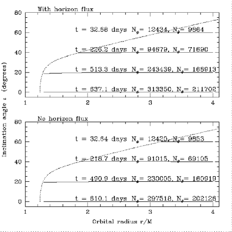
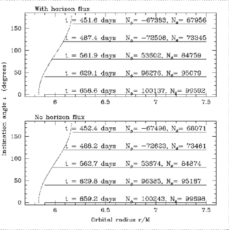
Figure 10: Inspiral trajectories for small bodies spiralling into massive, rotating black hole holes. These trajectories assume that the large black hole has mass $M=10^{6}\,M_{\odot}$ and that the small body is $1\,M_{\odot}$. The trajectories on the left are for spiral into a black hole with spin $a=0.998M$ (a near maximally spinning hole); those on the right are a hole with $a=0.05M$. Each point represents a possible circular orbit, with radius $r$ and inclination to the black hole’s equator $\iota$. Dotted lines show the innermost stable circular orbit: orbits below and to the right of the dotted line are stable, while those above and to the left are unstable, tending to plunge into the black hole. Gravitational waves drive the small body to spiral through a sequence of circular orbits. We show the time it takes the body to spiral to the innermost stable orbit, the number of orbits, $N_{\phi}$, executed as it does so, and the accumulated number of oscillations in $\theta$, $N_{\theta}$. In each figure, the top and bottom panels compare inspiral with the influence of the hole’s event horizon included (top) versus ignored (bottom).

The black hole nature of a massive object influences the inspiral of a small body in other ways. Fig. 10 shows the “trajectories” in radius $r$ and inclination angle $\iota$ followed by a $1\,M_{\odot}$ body that spirals into a $10^{6}\,M_{\odot}$ black hole. These trajectories were computed by studying how the energy and angular momentum of the orbit evolve due to losses from gravitational wave emission; see hughes_circI ; hughes_circII for details. In the top panels, gravitational waves carry energy and angular momentum both out to infinity and down the hole’s event horizon. In the lower panels, the horizon flux is ignored. When the hole is rapidly spinning, the horizon flux has an enormous influence on the inspiral, increasing the inspiral by several weeks and adding thousands of additional orbits. That the horizon flux increases the inspiral duration is at first sight counterintuitive — one would guess that the horizon is a sink for the orbit’s energy, and so its influence should decrease the inspiral duration. In fact, the hole supplies orbital energy: if it were not for the loss of energy in radiation carried to infinity, the body would spiral outward, rather than inward! This surprising behavior can be understood as either a tidal interaction between the small body and the event horizon, or as due to radiation that superradiantly scatters from the ergosphere of the black hole; see Refs. hughes_circII ; teuk_press ; hartle for further discussion. When the hole does not rotate rapidly, the effect is far smaller, and is more intuitively acceptable: orbital energy is lost to the black hole. Rapidly rotating black holes, if supplied to us by nature, will be particularly interesting laboratories for probing strong field gravity.

V.3 Dense nuclear matter and gravitational waves

Black holes are purely vacuum solutions to Einstein’s equations. Other gravitational-wave sources contain dense matter concentrations. In particular, neutron star sources are among the most studied for gravitational-wave detectors. A typical neutron star consists of approximately $1.5\,M_{\odot}$ of material with mean density $\rho\sim 10^{14}$ grams per cubic centimeter; such a star has a radius of 10 – 15 kilometers. The properties of that matter can have a large influence on the gravitational waves that neutron star systems generate. Thus gravitational-wave measurements from such systems may be used to study highly dense matter. Just a few measurements are needed to strongly constrain the equation of state of neutron star matter lindblom_eos . In this subsection, we briefly describe some examples of how this may be done.

When a neutron star is a member of a binary, the details of its nuclear matter structure are entirely irrelevant to gravitational-wave generation over much of the inspiral. It is only when the members of the binary are close enough that their tidal gravitational fields begin to distort one another that neutron star structure becomes potentially important. For double neutron star binaries, this means that the very late inspiral and merger waves (when the neutron stars collide and fuse into a single body) will depend quite strongly upon the properties of dense nuclear matter. Unfortunately, these waves are at very high frequencies ($\sim 1000$ Hz) where gravitational-wave detectors do not have good sensitivity. Special high frequency laser interferometers gdsw ; meers ; vmmb ; klm ; mizunoetal and acoustic detectors merk_johnson ; hsp can be used to improve our ability to measure these waves last3min ; hughes_thesis .

Better accuracy may be achieved by measuring waves from the coalescence of a black hole-neutron star binary. If the black hole is more massive than roughly $10\,M_{\odot}$, the neutron star will essentially be swallowed whole by the black hole. This is because the radii of the innermost orbits scale with the hole’s mass, and because the tidal field of the black hole scales as $M/r^{3}\sim 1/M^{2}$. Hence when the hole is large, its tides are relatively gentle and the neutron star can survive inspiral all the way through the hole’s event horizon. When the hole is smaller, however, the tides rip the neutron star apart before any matter falls down the horizon. This drastically changes the binary’s mass distribution and significantly affects its gravitational-wave emission. Because a black hole-neutron star system is significantly more massive than a double neutron star system, the waves that depend upon the neutron star’s matter are emitted at lower frequencies where laser interferometers have better sensitivity. Vallisneri vallis has shown that planned upgrades to LIGO will make it possible to extract a fair amount of information about neutron star properties by measuring such disruptions. However, he cautions that better theoretical modeling of the waves’ characteristics will be needed to fully understand what the detectors measure.

Neutron stars may undergo phase transitions as dense material changes state, perhaps forming a condensation of strange matter or free quark matter glendenning . If this occurs, the star’s density profile will rapidly change; any gravitational waves that it might be emitting will rapidly change character as well. This may be seen by following the waves that are emitted by an accreting neutron star chengdai : matter dumped onto the neutron star increases its mass beyond the critical point, until the phase transition occurs. The star then changes radius rapidly, exciting radial vibrational modes in the star. Other work suggests that such a phase transition may be see in the waves that are emitted as a neutron star forms during supernova collapse stm , changing the character of the star’s various oscillational modes. Finally, we note that a transition to such a form of nuclear matter has a drastic effect on the viscosity of material by changing the kinds of interactions that occur between nucleons in the star. This may cause various instabilities, particularly that due to r-modes, to damp out rapidly jones_prd ; jones_prl ; owen_lindblom . Gravitational-wave generation by neutron star systems present great opportunities for studying extremely dense matter, but as Vallisneri has emphasized, many theoretical uncertainties must be hammered out before we will be able to do so well.

V.4 Tests of new physics

Finally, gravitational waves will test current ideas for new unification physics beyond the standard-model-plus-GR paradigm. The best models for fundamental unification, based on string theory, lead to the idea that gravity propagates in more than three spatial dimensions. This has led to the investigation of “brane worlds”, in which standard model fields live on a 3D “brane” or boundary of a larger space (“bulk”) with one or more small or highly-curved extra dimensions akama ; holdom ; rub_shap ; add ; aadd ; randallsundrum1 ; randallsundrum2 . In these worlds, gravitons can have massive “Kaluza-Klein” modes that might be produced in accelerators, or survive from the early universe as dark matter. Even the massless modes, classical gravitational waves, no longer necessarily obey the same causal structure as electromagnetic waves; they can propagate either above or below the speed of light chung_freese ; ishihara ; ceg ; hebecker_marchrussell ; moffatt ; youm ; caldwelllanglois .

The possibility that a graviton might travel slower than a photon appears to be very tightly constrained by the fact that ultra high energy cosmic rays do not appear to lose energy to gravitational Čerenkov radiation moorenelson . However, in brane worlds, gravitons could also propagate faster than the speed of light. One can think of the extra dimensions as a kind of waveguide for the gravitational waves, so that the propagation is nondispersive; however, the curvature of the extra dimensions can also allow for faster propagation. We have little empirical information about this possibility at present, since we know only that the right amount of gravitational wave power is being emitted from binary pulsars. With LISA we will have coherent streams of gravitational waves from identified compact white-dwarf binaries that also have optically measured orbital parameters and orbital phases. The optical and gravitational wave data can be compared over many orbits, yielding a direct test of the propagation speed of gravitational waves that should be very precise.

These data will also constrain the possibility that the graviton is a composite particle, with components of more than one (possibly nonzero, but very small) mass. Classically emitted waves may, after propagating a large distance, separate out into two or more components. We might see a “standard” waveform of reduced amplitude, corresponding to the massless mode, with the rest of the energy appearing in some other, more dispersive waveform (or perhaps so highly delayed that it is not seen at all).

While we have discussed these programs in the context of concrete brane world models, it is possible to motivate them in more general language, as tests of Lorentz symmetry peters ; colemanglashow ; steckerglashow . The proliferation of unification ideas certainly justifies such an empirical approach; the detection of a cosmological constant has opened up consideration of an enormous range of mass scales so it has become interesting to constrain even what used to seem outrageously small masses.

Cosmology provides another context in which gravitational wave detectors will constrain fundamental physics. Generally, the connection comes through the possibility of generating a stochastic background of gravitational waves in the early universe that can be detected today maggiore . Gravitational-wave observatories will have an interesting sensitivity to these backgrounds; both LIGO and LISA will be able to detect broad-band stochastic backgrounds with energy densities well below the microwave background hoganbender ; bruceleshouches .

The source most often considered for such a background is cosmological inflation. We now think that parametrically-amplified quantum fluctuations of the inflaton field are responsible for large scale structure in the universe, and also for most of the fluctuation power in the microwave background anisotropy. The model predicts that similar fluctuations in the graviton field will produce a gravitational wave background. It is possible that these tensor waves are already contributing to the detected microwave anisotropy on the largest scales, and indeed there are experiments to test this possibility using the different polarization signatures of the anisotropy produced by the two kinds of modes.

These experiments are clearly important, but it will not be surprising if the tensor component turns out to be negligible. There is no reason for it to be comparable to the scalar (inflaton produced) component, as it depends on different parameters of the inflation model. (Indeed, the pure-scalar model with a scale-invariant spectrum fits the anisotropy data so well we would be disappointed to spoil it by adding another component with extra parameters.) The likely outcome is that the polarization experiments will constrain the tensor component, thereby constraining directly the expansion rate during inflation.

Even if the tensor component is detectable on the largest scales, the corresponding gravitational wave energy density for a scale-free spectrum (about $10^{-10}$ of the critical density at low frequencies, changing to $10^{-10}$ of the microwave energy density at high frequencies) is far too low for LIGO or LISA to detect directly. In some models, where the expansion rate increased to nearly the Planck scale during the course of inflation, the spectrum can be tilted enough to produce a detectable background, but these models are already ruled out by millisecond pulsar timing (which limits stochastic backgrounds to less than $10^{-3}$ of the microwave background density at frequencies of the order of inverse years) kaspi_taylor_ryba ; thorsett_dewey . Therefore it seems unlikely that the quantum graviton background will be seen by these observatories.

Some models however predict an entirely different source of primordial backgrounds. After inflation, the early universe may have hosted violent classical events that gave rise to a stochastic background. These gravitational waves could be much more intense than the inflationary quantum graviton production; the maximal energy density, limited by equipartition arguments, is approximately the same as the microwave background energy density— ten orders of magnitude above the typical inflationary level.

There are a number of circumstances which might approach within a few orders of magnitude of the maximal level. For example, a strongly first-order phase transition would lead to bubble nucleation and relativistic flows on the Hubble scale witten ; hogan_mnras ; kkt ; condensation of brane in a higher-dimensional space would lead to Kibble excitation of tensor modes on the Hubble scale hogan_prl ; hogan_prd . Strong effects of this kind are not required in any well established theory, but they are generic behaviors of relativistic systems that are worth constraining.

Backgrounds from these events are not scale-free; they tend to be broad band, but they have a characteristic frequency given by the redshifted Hubble rate. For detection at LISA and LIGO frequencies, the corresponding cosmic temperature turns out to be upwards of TeV energies— a range of interest for unification and supersymmetry breaking. This is a period of cosmic history about which we have almost no empirical information at present, so even upper limits from gravitational wave observatories will convey new information about physics at these energies. A detection would open up a new period of cosmic history to detailed scrutiny; we might for example find much more detailed information about the process of cosmic baryogenesis. The “last scattering surface” for gravitational waves is just their production epoch (that is, there is almost no significant absorption or large-angle scattering since the Planck time) so they provide a direct window into the early universe much deeper than the microwave background, and down to much smaller comoving scales. If a detectable stochastic background does exist, future generations of detectors may one day measure anisotropy in the background that contains new information about the early universe — a directly-imaged view of events invisible (even in principle) in any other way.

- (1) D. Kennefick, “Controversies in the History of the Radiation Reaction Problem in General Relativity”, unpublished Ph. D. thesis (Part II), California Institute of Technology (1997).
- (2) A. Einstein, Königlich Preußische Akademie der Wissenschaften Berlin, Sitzungsberichte, 154 (1918).
- (3) A. Einstein, Königlich Preußische Akademie der Wissenschaften Berlin, Sitzungsberichte, 688 (1916).
- (4) A. Abramovici et al., Science 256, 325 (1992).
- (5) K. S. Thorne, in 300 years of Gravitation, eds. S. W. Hawking and W. Israel (Cambridge University Press, Cambridge, 1987), p. 330.
- (6) R. Narayan, T. Piran, and A. Shemi, Astrophys. J. 379, L17 (1991)
- (7) E. S. Phinney, Astrophys. J. 380, L17 (1991)
- (8) V. Kalogera and D. R. Lorimer, Astrophys. J. 530, 890 (2000).
- (9) R. Weiss, Quarterly Progress Report of RLE, MIT 105, 54 (1972).
- (10) R. W. P. Drever, in Gravitational Radiation, eds. N. Deruelle and T. Piran (North Holland, Amsterdam, 1983).
- (11) Yu. Levin, Phys. Rev. D 57, 659 (1998).
- (12) Y. T. Liu and K. S. Thorne, Phys. Rev. D 62, 122002 (2000).
- (13) D. H. Santamore and Yu. Levin, Phys. Rev. D 64, 042002 (2001).
- (14) A. Buonanno and Y. Chen, Phys. Rev. D 64, 042006 (2001).
- (15) F. Marion, in Proceedings of the 3rd Edoardo Amaldi Conference, edited by S. Meshkov (AIP Conference Proceedings 523, Melville, New York, 2000), p. 110.
- (16) H. Lück et al., in Proceedings of the 3rd Edoardo Amaldi Conference, edited by S. Meshkov (AIP Conference Proceedings 523, Melville, New York, 2000), p. 119.
- (17) M. Ando et al., Phys. Rev. Lett. 86, 3950 (2001).
- (18) K. S. Thorne, “The Scientific Case for Mature LIGO interferometers,” LIGO Technical Report LIGO-P000024-00-R, Caltech/MIT, November 2000.
- (19) Gravitational-wave strain sensitivies are usually quoted with units . This is because the squared strain noise in a band is given by ; the final strain noise is thus dimensionless. The noise spectrum is often denoted .
- (20) K. Kuroda et al., Int. J. Mod. Phys. D 8, 557 (2000).
- (21) D. E. McCleland et al., in Proceedings of the 3rd Edoardo Amaldi Conference, edited by S. Meshkov (AIP Conference Proceedings 523, Melville, New York, 2000), p. 140.
- (22) S. A. Hughes and K. S, Thorne, Phys. Rev. D 58, 122002 (1998).
- (23) T. Creighton, Phys. Rev. D, submitted; gr-qc/0007050.
- (24) R. A. Hulse and J. H. Taylor, Astrophys. J. 195, L51 (1975).
- (25) J. H. Taylor and J. M. Weisberg, Astrophys. J. 345, 434 (1989).
- (26) H. Bethe and G. E. Brown, Astrophys. J. 506, 780 (1998).
- (27) C. L. Fryer, S. E. Woosley, and D. H. Hartmann, Astrophys. J. 526, 152 (1999).
- (28) K. Belczynski and T. Bulik, Astron. Astrophys. 346, 91 (1999).
- (29) S. F. Portegies-Zwart and L. R. Yungel’son, Astron. Astrophys. 332, 173 (1998).
- (30) S. F. Portegies-Zwart and S. L. W. McMillan, Astrophys. J. 528, L17 (2000).
- (31) E. E. Flanagan and S. A. Hughes, Phys. Rev. D 57, 4535 (1998).
- (32) B. Allen, in Proceedings of the Les Hourches School on Astrophysical Sources of Gravitational Waves, edited by J.-A. Marck and J.-P. Lasota (Cambridge University Press, Cambridge, 1996); gr-qc/9504033.
- (33) B. Allen and J. D. Romano, Phys. Rev. D 59, 102001.
- (34) E. Gustafson, D. Shoemaker, K. Strain, and R. Weiss, LSC White Paper on Detector Research and Development, LIGO Document T990080-00-D (1999).
- (35) C. Cutler and E. E. Flanagan, Phys. Rev. D 49, 2658 (1994).
- (36) B. J. Owen, Phys. Rev. D 53, 6749 (1996).
- (37) M. S. Turner, Phys. Rev. D 55, 45 (1997).
- (38) C. L. Fryer, D. E. Holz, and S. A. Hughes, Astrophys. J., in press; astro-ph/0106113.
- (39) P. R. Brady, T. Creighton, C. Cutler, and B. F. Schutz, Phys. Rev. D 57, 2101 (1999).
- (40) P. R. Brady and T. Creighton, Phys. Rev. D 61, 082001 (2000).
- (41) N. Andersson, Astrophys. J. 502, 708 (1998).
- (42) J. L. Friedman and S. M. Morsink, Astrophys. J. 502, 714 (1998).
- (43) L. Lindblom, B. J. Owen, and S. M. Morsink, Phys. Rev. Lett. 58, 084020 (1998).
- (44) N. Andersson, K. Kokkotas, and B. F. Schutz, Astrophys. J. 510, 846 (1999).
- (45) B. J. Owen, L. Lindblom, C. Cutler, B. F. Schutz, A. Vecchio, and N. Andersson, Phys. Rev. D 58, 084020 (1998).
- (46) L. Bildsten, Astrophys. J. 501, L89 (1998).
- (47) G. Ushomirsky, L. Bildsten, and C. Cutler, in Gravitational waves: Third Edoardo Amaldi Conference, edited by Sydney Meshkov, AIP Conference Proceedings No. 523 (American Institute of Physics, Melville, New York, 2000), p. 65.
- (48) LISA Pre-Phase A Report, 2nd Edition, edited by K. Danzmann, (Report MPQ-233, Max-Planck Institut für Quantenoptik, Garching, Germany), pp. 1-191 (1998).
- (49) Proceedings of the First International LISA Symposium: Class. Quant Grav. 14, 1397 – 1585 (1997).
- (50) Laser Interferometer Space Antenna, Proceedings of the 2nd LISA Symposium, AIP Conf. Proc. 456, edited by W. M. Folkner (American Institute of Physics, Woodbury, N. Y.), 3–239 (1998).
- (51) P. L. Bender, LISA: A Proposed Joint ESA-NASA Gravitational Wave Mission, in Gravitational Waves, edited by I. Ciufolini, V. Gorini, V. Moschella, and P. Fre (Institute of Physics Publishing, Bristol, UK), 115–151 (2001).
- (52) G. D. Quinlan and S. L. Shapiro, Astrophys. J. 343, 725 (1989); 356, 483 (1990).
- (53) M. G. Haehnelt and M. J. Rees, Mon. Not. R. Astron. Soc. 263, 168 (1993).
- (54) J. E. Tohline, R. H. Durisen and M. McCollough, Astrophys. J. 298, 220, 1985.
- (55) R. H. Durisen, R. A. Gingold, J. E. Tohline and A. P. Boss, Astrophys. J. 305, 281, 1986.
- (56) H. A. Williams and J. E. Tohline, Astrophys. J. 334, 449, 1988.
- (57) J. L. Houser, J. M. Centrella and S. Smith, Phys. Rev. Lett. 72, 1314, 1994.
- (58) S. Smith, J. L. Houser and J. M. Centrella, Astrophys. J. 458, 236 (1996).
- (59) J. L. Houser and J. M. Centrella, Phys. Rev. D 54, 7278 (1996).
- (60) B. K. Pickett, R. H. Durisen and R. H. Davis, Astrophys. J. 458, 714 (1996).
- (61) J. L. Houser, Mon. Not. R. Astro. Soc. 209, 1069 (1998).
- (62) K. C. B. New, J. M. Centrella and J. E. Tohline, Phys. Rev. D 62, 064019 (2000).
- (63) Y. T. Liu and L. Lindblom, Mon. Not. R. Astron. Soc. 324, 1063 (2001).
- (64) Y. T. Liu, Phys. Rev. D, submitted; gr-qc/0109078.
- (65) Y. T. Liu, private communication.
- (66) M. H. van Putten, Physics Reports 345, 1 (2001).
- (67) C. W. Misner, K. S. Thorne, and J. A. Wheeler, Gravitation (Freeman, San Francisco, 1973).
- (68) R. M. Wald, General Relativity (University of Chicago Press, Chicago, 1984).
- (69) S. A. Hughes, Mon. Not. R. Astron. Soc., submitted; astro-ph/0108483.
- (70) J. W. Armstrong, F. B. Estabrook, and M. Tinto, Astrophys. J. 527, 814 (1999).
- (71) C. J. Hogan and P. L. Bender, Phys. Rev. D 64, 062002 (2001).
- (72) R. Apreda, M. Maggiore, A. Nicolis, A. Riotta, gr-qc/0107033.
- (73) L. Blanchet, B. R. Iyer, A. G. Wiseman, and C. M. Will, Class. Quant. Grav. 13, 575 (1996).
- (74) I. H. Stairs, S. E. Thorsett, J. H. Taylor, and Z. Arzoumanian, in Pulsar Astronomy — 2000 and Beyond, ASP Conference Series, Vol. 202 (ASP, San Francisco, 2000).
- (75) I. H. Stairs et al., Astrophys. J. 505, 352 (1998).
- (76) T. Damour and J. H. Taylor, Astrophys. J. 366, 501 (1991).
- (77) S. A. Teukolsky, Astrophys. J. 185, 635 (1973).
- (78) E. W. Leaver, Proc. R. Soc. Lond. A402, 285 (1985).
- (79) F. Echeverria, Phys. Rev. D 40, 3194 (1989).
- (80) A recent review of numerical relativity is L. Lehner, Class. Quant. Grav. 18, R25 (2001); gr-qc/0106072.
- (81) N. T. Bishop, R. Gómez, L. Lehner, and J. Winicour, Phys. Rev. D 54, 6153 (1996).
- (82) L. E. Kidder, M. A. Scheel, and S. A. Teukolsky, Phys. Rev. D 64, 064017 (2001).
- (83) J. Baker, M. Campanelli, and C. O. Lousto, gr-qc/0104063.
- (84) J. Baker, B. Brügmann, M. Campanelli, C. O. Lousto, and R. Takahashi, Phys. Rev. Lett. 87, 121103 (2001).
- (85) A. Buonnano and T. Damour, Phys. Rev. D 49, 084006 (1999).
- (86) T. Damour, gr-qc/0103018.
- (87) E. Poisson, Phys. Rev. D 47, 1497 (1993).
- (88) C. Cutler, D. Kennefick, and E. Poisson, Phys. Rev. D 50, 3816 (1994).
- (89) Y. Mino, M. Sasaki, M. Shibata, H. Tagoshi, and T. Tanaka, Prog. Theor. Phys. Suppl. No. 128, Chapter 1 (1997).
- (90) S. A. Hughes, Phys. Rev. D 61, 084004 (2000); 63, 049902(E) (2001).
- (91) S. A. Hughes, Phys. Rev. D 64, 064004 (2001)
- (92) D. Kennefick and K. Glampdakis, in preparation.
- (93) D. Merritt and L. Ferrarese, to appear in The Central Kpc of Starbursts and AGN, edited by J. H. Knapen, J. E. Beckman, I. Shlosman and T. J. Mahoney; astro-ph/0107134.
- (94) F. Ryan, Phys. Rev. D 56, 1845 (1997).
- (95) The term “bothrodesy” has been coined by Sterl Phinney. It descends from the use of the suffix “-bothron” introduced by Brandon Carter to describe properties of black holes. This suffix, in turn, descends from the Greek word “”, meaning “garbage dump”.
- (96) S. A. Teukolsky and W. H. Press, Astrophys. J. 193, 443 (1974).
- (97) J. B. Hartle, Phys. Rev. D 8, 1010 (1973); 9, 2749 (1974).
- (98) L. Lindblom, Astrophys. J. 398, 569 (1992).
- (99) B. J. Meers, Phys. Rev. D 38, 2317 (1988).
- (100) J.-Y. Vinet, B. J. Meers, C. N. Man, and A. Brillet, Phys. Rev. D 38, 433 (1988).
- (101) A. Królak, K. A. Lobo, and B. J. Meers, Phys. Rev. D 43, 2470 (1991).
- (102) J. Mizuno et al., Phys. Lett. A 175, 273 (1993).
- (103) S. M. Merkowitz and W. W. Johnson, Phys. Rev. D 51, 2546 (1995).
- (104) G. M. Harry, T. R. Stevenson, and H. J. Paik, Phys. Rev. D 54, 2546 (1996).
- (105) C. Cutler et al., Phys. Rev. Lett. 70, 2984 (1993).
- (106) S. A. Hughes, in preparation; preliminary version available as Chapter 4 of S. A. Hughes, “Gravitational-wave astronomy: Aspects of the theory of binary sources and interferometric detectors”, unpublished Ph. D. thesis, California Institute of Technology (1998).
- (107) M. Vallisneri, Phys. Rev. D 84, 3519 (2000).
- (108) N. K. Glendenning, Compact Stars (Springer, New York, 2000).
- (109) K. S. Cheng and Z. G. Dai, Astrophys. J. 492, 281 (1998).
- (110) H. Sotani, K. Tominaga, and K. Maeda, gr-qc/0108060.
- (111) P. B. Jones, Phys. Rev. D 64, 084003 (2001).
- (112) P. B. Jones, Phys. Rev. Lett. 86, 1384 (2001).
- (113) B. J. Owen and L. Lindblom, in preparation.
- (114) K. Akama, Lect. Notes Phys. 176, 267 (1982); hep-th/0001113.
- (115) B. Holdom, ITP-744-STANFORD.
- (116) V. A. Rubakov and M. E. Shaposhnikov, Phys. Lett. B 125, 136 (1983).
- (117) N. Arkani-Hamed, S. Dimopoulos, and G. Dvali, Phys. Lett. B 429, 263 (1998); hep-ph/9803315.
- (118) I. Antoniadis, N. Arkani-Hamed, S. Dimopoulos, and G. Dvali, Phys. Lett. B 436, 257 (1998); hep-ph/9804398.
- (119) L. Randall and R. Sundrum, Phys. Rev. Lett. 83, 3370 (1999); hep-ph/9905221.
- (120) L. Randall and R. Sundrum, Phys. Rev. Lett. 83, 4690 (1999); hep-th/9906064.
- (121) D. J. H. Chung and K. Freese, Phys. Rev. D 61, 023511 (2000); hep-ph/9906542.
- (122) H. Ishihara, Phys. Rev. Lett. 86, 381 (2001); gr-qc/0007070.
- (123) C. Csaki, J. Erlich, and C. Grojean, Nucl. Phys. B 604, 312 (2001); hep-th/0012143.
- (124) A. Hebecker and J. March-Russell, Nucl. Phys. B 608, 375 (2001); hep-ph/0103214.
- (125) J. W. Moffat, hep-th/0105017.
- (126) D. Youm, hep-th/0102194.
- (127) R. R. Caldwell and D. Langlois, Phys. Lett. B 511, 129 (2001); gr-qc/0103070.
- (128) G. D. Moore and A. E. Nelson, hep-ph/0106220.
- (129) P. C. Peters, Phys. Rev. D 9, 2207 (1974).
- (130) S. Coleman and S. L. Glashow, Phys. Rev. D 59, 116008 (1999); hep-ph/9812418.
- (131) F. W. Stecker and S. L. Glashow, Astropart. Phys. 16, 97 (2001); astro-ph/0102226.
- (132) M. Maggiore, Phys. Rep. 331, 283 (2000).
- (133) B. Allen, in Proceedings of the Les Houches School on Astrophysical Sources of Gravitational Waves, eds. J.-A. Marck and J.-P. Lasota (Cambridge University Press, Cambridge, 1996); gr-qc/9604033.
- (134) V. Kaspi, J. H. Tayor, and M. F. Ryba Astrophys. J. 428, 713 (1999).
- (135) S. Thorsett, R. Dewey Phys. Rev. D 53, 3498 (1996).
- (136) E. Witten, Phys. Rev. D 30, 272 (1984).
- (137) C. J. Hogan, Mon. Not. R. Astron. Soc. 218, 629 (1986).
- (138) M. Kamionkowski, A. Kosowsky, and M. S. Turner, Phys. Rev. D 49, 2837 (1994).
- (139) M. Gleiser and R. Roberts, Phys. Rev. Lett. 81, 5497 (1998).
- (140) C. J. Hogan, Phys. Rev. Lett. 85, 2044 (2000).
- (141) C. J. Hogan, Phys. Rev. D 62, 121302 (2000).