Cosmic Structure Formation with Topological Defects

1 Introduction

Topological defects are ubiquitous in physics. Whenever a symmetry breaking phase transition occurs, topological defects may form. The best known examples are vortex lines in type II super conductors or in liquid Helium, and declination lines in liquid crystals [109, 24]. In an adiabatically expanding universe which cools down from a very hot initial state, it is quite natural to postulate that topological defects may have emerged during a phase transition in the early universe and that they may have played the role of initial inhomogeneities seeding the formation of cosmic structure. This basic idea goes back to Kibble (1976) [88]. In this report we summarize the progress made in the investigation of Kibble’s idea during the last 25 years. Our understanding of the formation and evolution of topological defects is reported almost completely in the beautiful book by Vilenkin & Shellard [152] or the excellent Review by Hindmarsh & Kibble [71], and we shall hence be rather short on that topic. Nevertheless, in order to be self contained, we have included a short chapter on spontaneous symmetry breaking and defect formation. Our main topic is however the calculation of structure formation with defects, results which are not included in [152] and [71].

Besides the formation of structure in the universe, topological defects may be relevant for the baryon number asymmetry of the universe [33]. Superconducting cosmic strings [159] or vortons [20] might produce the high energy cosmic rays [15], or even gamma ray bursts [12]. The brane worlds which have have focussed a lot of attention recently, may actually just represent topological defects in a higher dimensional space [65, 61, 62]. There have also been interesting results on chiral strings and their observational signatures [21, 138]. GUT scale cosmic strings could be detected by their very peculiar lensing properties. For a straight cosmic string lensing is very simple [152]. For a more realistic network of strings, characteristic caustics and cusps in the lensing signal are very generically expected [96, 148, 14].

The relevant energy scale for a topological defect is $T_{c}$, the phase transition temperature. Hence a good estimate for the amplitude of the dimensionless gravitational potential $\Psi$ induced by topological defects is

$$\Psi\sim 4\pi GT_{c}^{2}=4\pi(T_{c}/M_{\rm P})^{2}~{},$$ (1)

where $M_{\rm P}$ denotes the Planck mass. The measurements of cosmic microwave background anisotropies on large scales by the cosmic background explorer (COBE) satellite [134] have found that this potential, which is of the same order as the temperature fluctuations on large scales, is about $10^{-5}$. Hence, for cosmic structure formation, we are interested in phase transitions at $T_{c}\sim 10^{-3}M_{\rm P}\sim 10^{16}$GeV. Interestingly, this is just the scale of the grand unification phase transition (GUT scale) of supersymmetric GUT’s (grand unified theories).

Topological defects represent regions in space-time where the corresponding field (order parameter in condensed matter physics or Higgs field in particle physics) is frustrated. It cannot relax into the vacuum state, the lowest energy state, by topological obstructions. They represent positions of higher energy density and are thus inherently inhomogeneous distributions of energy and momentum. We shall discuss concrete examples later.

In the remainder of this introduction we give a brief overview of the problem of structure formation and we present the main results worked out in this report.

In Chapter 2 we introduce the concept of topological defect formation during symmetry breaking phase transitions, we classify the defects and illustrate them with examples.
In Chapter 3 we present in detail the theoretical framework used to investigate structure formation with topological defects. This chapter together with two appendices is self contained and should enable a non-specialist in the field to fully understand the often somewhat sketchy literature.
In Chapter 4 we discuss numerical simulation of topological defects. We distinguish global and local defects which have to be treated in a very different way. We specify the approximations made in different numerical implementations and discuss their validity and drawbacks.
In Chapter 5 we present the results of simulations of structure formation with topological defects and compare them with present observations.
In Chapter 6 we investigate the question in whether the results discussed in Chapter 5 are generic or whether they are just special cases. We derive properties of the unequal time correlators of generic causal scaling seeds. Since these are the sole ingredients in the calculation of the fluctuation power spectra, they determine the ’phase space’ of defect models of structure formation. We discuss a model of causal scaling seeds which mimics the cosmic microwave background (CMB) anisotropy spectrum of inflation. We also consider the possibility that large scale structure may be due to a mixture of adiabatic inflationary initial perturbations and topological defects. We study especially the fluctuations in the CMB. We investigate to which extent CMB parameter estimations are degraded if we allow for an admixture of defects.

We end with a brief summary of the main results.

Throughout this work we use units with $c=\hbar=k_{\rm Boltzmann}=1$. The basic unit is thus either an energy (we usually take MeV’s) or a length, for which we take cm or Mpc depending on the situation.
We choose the metric signature $(-,+,+,+)$. Three-dimensional vectors are denoted in boldface. The variables $x$ and $k$ are comoving position and comoving wave vector in Fourier space. Greek indices, $\mu,\nu,\cdots$ denote spacetime components of vectors and tensors while Latin indices $i,j,\cdots$ denote three dimensional spatial components. We mostly use conformal time $\tau$ with $d\tau=dt/a$, where $t$ is cosmic time and $a$ is the scale factor. Derivatives with respect to conformal time are indicated by an over-dot, $\dot{f}={df\over d\tau}$.

1.1 Main results

Before we start to discuss models of structure formation with topological defects in any detail, let us present the main results discussed in this review.

We concentrate primarily on CMB anisotropies. Since these anisotropies are small, they can be calculated (almost fully) within linear cosmological perturbation theory. To compare models with other data of cosmic structure, like the galaxy distribution or velocities, one has to make some assumptions concerning the not well understood relation between the distribution of galaxies and of the dark matter, the problem of biasing. Furthermore, on small scales one has to study non-linear Newtonian clustering which is usually done by $N$-body simulations. But to lay down the initial conditions for $N$-body simulations, one does not only need to know the linear power spectrum, but also the statistical distribution of the fluctuations which is largely unknown for topological defects. Fluctuations induced by topological defects are generically non-Gaussian, but to which extent and how to characterize their non-Gaussianity is still an open question. In this report, we therefore concentrate on CMB anisotropies and their polarization and shall only mention on the side the induced matter fluctuations and bulk velocities on large scales.

Like inflationary perturbations, topological defects predict a Harrison-Zel’dovich spectrum of perturbations [69, 163]. Therefore, the fluctuation spectrum is in good agreement with the COBE DMR experiment [134], which has measured CMB anisotropies on large angular scales and found that they are approximately constant as expected from a Harrison-Zel’dovich spectrum of initial fluctuations (see e.g.  [113]).

Since quite some time it is known, however, that topological defect differ from adiabatic inflationary models in the acoustic peaks of the CMB anisotropy spectrum [44]. Due to the isocurvature nature of defects, the position of the first acoustic peak is shifted from an angular harmonic of about $\ell\sim 220$ to $\ell\sim 350$ (or up to $\ell\sim 500$ in the case of cosmic strings) for a spatially flat universe. More important, the peaks are much lower in defect models and they are smeared out into one broad hump with small wiggles at best. Even by changing cosmological parameters at will, this second characteristics cannot be brought in agreement with present CMB anisotropy data like [110, 66, 97]. Also the large scales bulk velocities, which measure fluctuation amplitudes on similar scales turn out to be too small [47].

As the CMB anisotropy signals from cosmic strings and from global $O(N)$ defects are quite different, it is natural to wonder how generic these results may be. Interestingly enough, as we shall see in Chapter 6, one can define ’scaling causal seeds’, i.e. initial perturbations which obey the basic constraints for topological defects and which show a CMB anisotropy spectrum resembling adiabatic inflationary predictions very closely [144]. This ’Turok model’ can nevertheless be distinguished from adiabatic perturbations by the CMB polarization spectrum. Also mixed models with a relatively high degree of defect admixture, up to more than 50%, are in good agreement with the data.

1.2 Cosmic structure formation

The geometry of our universe is to a very good approximation isotropic and therefore (if we assume that we are not situated in a special position) also homogeneous. The best observational evidence for this fact is the isotropy of the cosmic microwave background which is (apart from the dipole anisotropy) on the level of about $10^{-5}$ – $10^{-4}$.

Nevertheless, on galaxy and cluster scales, the matter distribution is very inhomogeneous. If these inhomogeneities have grown by gravitational instability from small initial fluctuations, the amplitude of the initial density fluctuations have to be about $10^{-4}$ to become of order unity or larger today. Radiation pressure inhibits growth of perturbations as long as the universe is radiation dominated, and even in a matter dominated universe small perturbations grow only like the scale factor.

The discovery of large angular scale fluctuations in the CMB by the DMR experiment aboard the COBE satellite [134], which are just about of the needed amplitude, is an important support of the gravitational instability picture. The DMR experiment also revealed that the spectrum of fluctuations is ’flat’, which means that the fluctuations have a fixed amplitude $A$ when entering the Hubble horizon. This implies that temperature fluctuations on large scales are constant, as measured by COBE:

$$\left\langle\left(\frac{\Delta T}{T}\right)^{2}(\vartheta)\right\rangle\simeq 10^{-10}=\mbox{ constant,}$$ (2)

independent of the angle $\vartheta$, for $\vartheta\gg 1^{o}$. These fluctuations are of the same order of magnitude as the gravitational potential. Their smallness therefore justifies the use of linear perturbation theory. Within linear perturbation theory, the gravitational potential does not grow. This observation originally led Lifshitz to abandon gravitational instability as the origin for cosmic structure [100]. But density fluctuations of dust can become large and can collapse to form galaxies and even black holes. At late times and on scales which are small compared to the horizon, linear perturbation theory is no longer valid and numerical N-body simulations have to be performed to follow the formation of structure. But also with N-body simulations one cannot compute the details of galaxy formation which strongly depend on thermal processes like cooling and formation of heavy elements in stars. Therefore, the relation of the power spectrum obtained by N-body simulations to the observed galaxy power spectrum may not be straight forward. This problem is known under the name of ’biasing’.

Within linear perturbation analysis, structure formation is described by an equation of the form

$${\cal D}X(\mbox{\boldmath$k$},\tau)={\cal S}(\mbox{\boldmath$k$},\tau)~{},$$ (3)

where $\cal D$ is a time dependent linear differential operator, $k$ is the wave vector and $X$ is a long vector describing all the cosmic perturbation variables for a given $k$-mode, like the dark matter density and velocity fluctuations, the CMB anisotropy multipole amplitudes and so on. ${\cal S}$ is a source term. In Chapter 3 we will write down the system (3) explicitly.

There are two basically different classes of models for structure formation. In the first class, the linear perturbation equations are homogeneous, i.e. ${\cal S}\equiv 0$, and the resulting structure is determined by the initial conditions and by the cosmological parameters of the background universe alone. Inflationary initial perturbations are of this type. In most models of inflation, the initial fluctuations are even Gaussian and the entire statistical information is contained in the initial power spectrum. The evolution is given by the differential operator $\cal D$ which depends on the cosmological parameters.

In the second class, the linear perturbation equations are inhomogeneous, having a so called source term or ’seed’, ${\cal S}$, on the right hand side which evolves non-linearly in time. Topological defects are of this second class. The difficulty of such models lies in the non-linear evolution of the seeds, which in most cases has to be determined by numerical simulations. Without additional symmetries, like e.g.   scaling in the case of topological defects, it is in general not possible to simulate the seed evolution over the long time-scale and for the considerable dynamical range needed in cosmology. We shall see in Chapter 4 how this problem is overcome in the case of topological defects. An additional difficulty of models with seeds is their non-Gaussian nature. Due to non-linear evolution, even if the initial conditions are Gaussian, the seeds are in general not Gaussian at late times. The fluctuation power spectra therefore do not contain the full information. All the reduced higher moments can be relevant. Unfortunately only very little work on these non-Gaussian aspects of seed models has been published and the results are highly incomplete [60, 43, 59].

2 Symmetry Breaking Phase Transitions and the Formation of Topological Defects

2.1 Spontaneous symmetry breaking

Spontaneous symmetry breaking is a concept which originated in condensed matter physics. As an example consider the isotropic model of a ferro-magnet: although the Hamiltonian is rotationally invariant, the ground state is not. The magnetic moments point all in the same direction.

In models of elementary particle physics, symmetry breaking is most often described in terms of a scalar field, the Higgs field. In condensed matter physics this field is called the order parameter. It can also be a vector or tensor field.

A symmetry is called spontaneously broken if the ground state is not invariant under the full symmetry of the Lagrangian (or Hamiltonian) density. Since the symmetry group can be represented as a group of linear transformations, this implies that the vacuum expectation value of the Higgs field is non-zero.

The essential features of a spontaneously broken symmetry can be illustrated with a simple model which was first studied by Goldstone (1961) [64]. This model has the classical Lagrangian density

$${\cal L}=\partial_{\mu}\bar{\phi}\partial^{\mu}\phi-V(\phi)~{}~{}\mbox{ with }~{}~{}~{}V={1\over 4}\lambda(|\phi|^{2}-\eta^{2})^{2}~{}.$$ (4)

Here $\phi$ is a complex scalar field and $\lambda$ and $\eta$ are real positive constants. The potential in (4) is called the ’Mexican hat potential’ as it looks somewhat like a Mexican sombrero. This Lagrangian density is invariant under the group $U(1)$ of global phase transformations,

$$\phi(x)\mapsto e^{i\alpha}\phi(x)~{}.$$ (5)

The minima of the potential $V$ lie on the circle $|\phi|=\eta$ which is called the ’vacuum manifold’, ${\cal M}={\bf S}_{\eta}^{1}$ (here and in what follows ${\bf S}^{n}_{R}$ denotes an $n$-sphere of radius $R$ and ${\bf S}^{n}$ denotes an $n$-sphere of radius $1$). The notion ’global’ indicates that the symmetry transformation is global, i.e., $\alpha$ is independent of the spacetime position $x$. The quantum ground states (vacuum states) $|0\rangle$ of the model are characterized by

$$\langle 0|\phi|0\rangle=\eta e^{i\beta}\neq 0~{}.$$ (6)

A phase transformation changes $\beta$ into $\beta+\alpha$, hence a ground state is not invariant under the symmetry transformation given in Eq. (5). (Clearly, the full vacuum manifold ${\cal M}$ is invariant under symmetry transformations and thus a mixed state which represents a homogeneous mixture of all vacuum states is still invariant even though no pure state is.) The only state $|u\rangle$ invariant under the symmetry (5), characterized by $\langle u|\phi|u\rangle=0$, corresponds to a local maximum of the potential. Small perturbations around this ’false vacuum’ have ’negative mass’ which indicates the instability of this state:

$$V(\phi)=-{1\over 2}\lambda\eta^{2}|\phi|^{2}+\mbox{const.}+{\cal O}(|\phi|^{4})~{}.$$ (7)

The vacuum states of the broken symmetry are all equivalent and we can thus reveal their properties by studying one of them. For convenience we discuss the vacuum state with vanishing phase, $\langle 0|\phi|0\rangle=\eta$. Expanding the field around this state yields

$$\phi(x)=(\eta+{1\over\sqrt{2}}\varphi(x))e^{i\vartheta(x)}~{},$$ (8)

where $\varphi$ and $\vartheta$ are real fields. The Lagrangian density in terms of $\varphi$ and $\vartheta$ becomes

$${\cal L}={1\over 2}\left(\partial_{\mu}\varphi\right)^{2}+\eta^{2}\left(\partial_{\mu}\vartheta\right)^{2}-{1\over 2}\lambda\eta^{2}\varphi^{2}+{\cal L}_{int}(\varphi,\vartheta)~{}.$$ (9)

The interaction Lagrangian ${\cal L}_{int}$ is easily determined from the original Lagrangian,  (4). This form of the Lagrangian shows that the degree of freedom $\varphi$ is massive with mass $m^{2}=\lambda\eta^{2}$ while $\vartheta$ describes a massless particle (circular excitations), a Goldstone boson. This simple model is very generic: whenever a continuous global symmetry is spontaneously broken, massless Goldstone bosons emerge. Their number equals the dimension of the vacuum manifold, i.e., the dimension of a group orbit (in the space of field values). In our case the space of field values is $\Cset\approx\Rset^{2}$. A group orbit is a circle of dimension $1$ leading to one massless boson, the excitations tangential to the circle which cost no potential energy. The general result can be formulated in the following theorem:

Theorem 1

(Goldstone, 1961) [64] If a continuous global symmetry, described by a symmetry group $G$ is spontaneously broken to a sub-group $H\subset G$, massless particles emerge. Their number is equal to the dimension $n$ of the vacuum manifold ${\cal M}$ (the “number of broken symmetries”). Generically,

$${\cal M}\equiv G/H~{}~{}~{}\mbox{ and }~{}~{}~{}~{}n=dimG-dimH=dim\left(G/H\right)~{},$$

where here $\equiv$ means topological equivalence.

In our example $G=U(1)$, $H=\{1\}$ and $n=1-0=1$.
Another well-known example are the three pions, $\pi^{\pm}$, $\pi^{0}$, which are the Goldstone bosons of isospin (proton/neutron) symmetry. There the original symmetry, $SU(2)$ is completely broken leading to $n=dimSU(2)=3$ Goldstone bosons (see. e.g.  [77]).

Very often, symmetries in particle physics are gauged (local). The simplest gauge theory is the Abelian Higgs model (sometimes also called scalar electrodynamics). It is described by the Lagrangian density

$${\cal L}=\overline{D}_{\mu}\bar{\phi}D^{\mu}\phi-V(\phi)-{1\over 4}F_{\mu\nu}F^{\mu\nu}~{},$$ (10)

where $\phi$ is again a complex scalar field and $D_{\mu}=\partial_{\mu}-ieA_{\mu}$ is the covariant derivative w.r.t. the gauge field $A_{\mu}$. $F_{\mu\nu}=\partial_{\mu}A_{\nu}-\partial_{\nu}A_{\mu}$ is the gauge field-strength, $e$ the gauge coupling constant and $V$ is the potential given in Eq. (4).

This Lagrangian is invariant under the group of local $U(1)$ transformations,

$$\phi\mapsto e^{i\alpha(x)}\phi(x)~{}~{},~{}~{}~{}~{}~{}~{}A_{\mu}(x)\mapsto A_{\mu}(x)+{1\over e}\partial_{\mu}\alpha(x)~{}.$$

The minima of the potential, $\phi=\eta e^{i\beta}$, are not invariant, the symmetry is spontaneously broken. Expanding as before around the vacuum expectation value $\langle 0|\phi|0\rangle=\eta$, we find

$${\cal L} = [\partial_{\mu}\varphi-(ieA_{\mu}+i\partial_{\mu}\vartheta)(\eta+\varphi)][\partial^{\mu}\varphi+(ieA^{\mu}+i\partial^{\mu}\vartheta)(\eta+\varphi)]$$ (11)

$$-{1\over 2}m^{2}\varphi^{2}-{1\over 2}\lambda\varphi^{4}-{1\over 4}F_{\mu\nu}F^{\mu\nu}~{},$$

where, as in the global case, $m^{2}=\lambda\eta^{2}$. Here $\vartheta$ is no longer a physical degree of freedom. It can be absorbed by a gauge transformation. After the gauge transformation $A_{\mu}\mapsto A_{\mu}-(1/e)\partial_{\mu}\vartheta$ the Lagrangian given in Eq. (11) becomes

$${\cal L}=(\partial_{\mu}\varphi)^{2}-{1\over 2}m^{2}\varphi^{2}+{1\over 2}M^{2}A_{\mu}A^{\mu}-{1\over 4}F_{\mu\nu}F^{\mu\nu}+{\cal L}_{int}~{},$$ (12)

with $m=\sqrt{\lambda}\eta$ and $M=\sqrt{2}e\eta$. The gauge boson “absorbs” the massless Goldstone boson and becomes massive. It has now three independent polarizations (degrees of freedom) instead of the original two. The phenomenon described here is called the ’Higgs mechanism’. It works in the same way also for more complicated non-Abelian gauge theories (Yang Mills theories).

On the classical level, what we have done here is just rewriting the Lagrangian density in terms of different variables. However, on a quantum level, particles are excitations of a vacuum state, a state of lowest energy, and these are clearly not described by the original field $\phi$ but by the fields $\varphi$ and $\vartheta$ in the global case and by $\varphi$ and $A_{i}$ in the local case.

The two models presented here have very close analogies in condensed matter physics:
a) The non-relativistic version of Eq. (4) is used to describe super fluids where $\phi$ is the Bose condensate (the best known example being super fluid He⁴).
b) The Abelian Higgs model, Eq. (10) is the Landau Ginzburg model of super-conductivity, where $\phi$ represents the Cooper pair wave function.

A very physical and thorough account of the problem of spontaneous symmetry breaking can be found in Weinberg [157].

It is possible that also the scalar fields in particle physics (e.g. the Higgs of the standard model which is supposed to provide the masses of the $W^{\pm}$ and $Z^{0}$) are not fundamental but “condensates” as in condensed matter physics. Maybe the fact that no fundamental scalar particle has been discovered so far has some deeper significance.

2.2 Symmetry restoration at high temperature

In particle physics like in condensed matter systems, symmetries which are spontaneously broken can be restored at high temperatures. The basic reason for this is that a system at finite temperature is not in the vacuum state which minimizes energy, but in a thermal state which tends to maximize entropy. We thus have to expand excitations of the system about a different state. More precisely, it is not the potential energy, but the free energy

$$F=E-TS$$ (13)

which has to be minimized. The equilibrium value of $\phi$ at temperature $T$, $\langle\phi\rangle_{T}$, is in general temperature dependent [90]. At low temperature, the entropy term is unimportant. But as the temperature raises, low entropy becomes more and more costly and the state tends to raise its entropy. The field $\phi$ becomes less and less ordered and thus its expectation value $\langle\phi\rangle_{T}$ becomes smaller. Above a certain critical temperature, $T\geq T_{c}$, the expectation value $\langle\phi\rangle_{T}$ vanishes. If the coupling constants are not extremely small, the critical temperature is of order $T_{c}\sim\eta$.

To calculate the free energy of quantum fields at finite temperature, one has to develop a perturbation theory similar to the $T=0$ Feynman diagrams, where ordinary Greens functions are replaced by thermal Greens functions. The inverse temperature, $\beta=1/(kT)$ plays the role of an imaginary time component. It would lead us too far from the main topic of this review to introduce thermal perturbation theory, and there are excellent reviews on the subject available, see, e.g. [11, 157, 86, 156, 39, 90].

Here we give a much simplified derivation of the lowest order (tree level) thermal correction to the effective potential [152]. In lowest order the particles are non-interacting and their contributions to the free energy can be summed (each degree of freedom describes one particle),

$$V_{\rm eff}(\phi,T)=V(\phi)+\sum_{n}F_{n}(\phi,T)~{}.$$ (14)

Here $V(\phi)$ is the zero temperature effective potential and $F_{n}$ is the free energy of each degree of freedom,

$$F_{n}=\pm\int{d^{3}k\over(2\pi)^{3}}\ln(1\mp\exp(-\epsilon(k)/T))~{},$$ (15)

as known from statistical mechanics. The upper sign is valid for bosons and the lower one for fermions. $\epsilon(k)=\sqrt{k^{2}+m_{n}^{2}}$.

For $T\ll m_{n}$ the free energy is exponentially small. But it can become considerable at high temperature, $T\gg m_{n}$, where we obtain

$$F_{n}=\left\{\begin{array}[]{ll}-{\pi^{2}\over 90}T^{4}+{m_{n}^{2}T^{2}\over 24}+{\cal O}(m_{n}^{4})&\mbox{bosons}\\ -{7\pi^{2}\over 720}T^{4}+{m_{n}^{2}T^{2}\over 48}+{\cal O}(m_{n}^{4})&\mbox{fermions.}\end{array}\right.$$ (16)

If symmetry restoration occurs at a temperature well above all the mass thresholds, we can approximate $V_{\rm eff}$ by

$$V_{\rm eff}(\phi,T)=V_{\rm eff}(\phi,T=0)+{1\over 24}{\cal M}^{2}T^{2}-{\pi^{2}\over 90}{\cal N}T^{4}~{},$$ (17)

$${\cal N}=N_{B}+{7\over 8}N_{F}~{},~{}~{}{\cal M}^{2}=\sum_{\rm bosons}m_{n}^{2}+{1\over 2}\sum_{\rm fermions}m_{n}^{2}~{}.$$ (18)

Here, $m_{i}$ is the formal mass given by $m_{i}^{2}={\partial^{2}V\over(\partial\phi^{i})^{2}}$. If the potential contains a $\phi^{4}$-term, the mass includes a term $\propto\phi_{i}^{2}$, which leads to a positive quadratic term, $\propto T^{2}\phi_{i}^{2}$. If the temperature is sufficiently high, this term overcomes the negative quadratic term in the Mexican hat potential and $\phi=0$ becomes a global minimum of the potential. The temperature at which this happens is called the critical temperature.

In the Abelian Higgs model, the critical temperature $T_{c}$, becomes [152]

$$T_{c}^{2}={6\lambda\eta^{2}\over\lambda+3e^{2}}~{}.$$ (19)

For non-Abelian $O(N)$ models one finds analogously [152]

$$T_{c}^{2}={6\lambda\eta^{2}\over{N+2\over 4}\lambda+3(N-1)e^{2}}~{}.$$ (20)

The critical temperature for global symmetry breaking, i.e. without gauge field, is obtained in the limit $e\rightarrow 0$. As expected, for $e^{2}\stackrel{{\scriptstyle<}}{{\sim}}\lambda$ one finds

$$T_{c}\sim\eta~{}.$$ (21)

Like in condensed matter systems, a phase transition is second order if $\phi=0$ is a local maximum and first order if $\phi=0$ is a local minimum. In the example of the Abelian Higgs model, the order depends on the parameters $e$ and $\lambda$ of the model.

In $O(N)$ models, or any other model where the vacuum manifold (i.e. the space of minima of the effective potential) of the broken symmetry phase is non-trivial, minimization of the effective potential fixes the absolute value of $\phi$ but the direction, $\phi/|\phi|$, is arbitrary. The field can vary in the vacuum manifold, given by the sphere ${\bf S}^{N-1}=O(N)/O(N-1)$ for $O(N)$ models. At low temperature, the free energy is minimized if the phase is constant (no gradient energy) but after the phase transition $\phi/|\phi|$ will vary in space. The size of the patches with roughly constant direction is given by the correlation length $\xi$ which is a function of time. In the early universe $\xi$ is bounded by the size of the causal horizon,

$$\xi(t)\leq d_{H}(t)\sim t~{}~{}~{}\mbox{ for power law expansion.}$$ (22)

Formally $\xi$ diverges at the phase transition, but also our perturbative treatment is no longer valid in the vicinity of the phase transition since fluctuations become big. A thorough treatment of the physics at the phase transition is the subject of modern theory of critical phenomena and goes beyond the scope of this review. Very often, the relevant correlation length is the correlation length at the Ginsburg temperature, $T_{G}$, the temperature at which thermal fluctuations are comparable to the mass term. However, in the cosmological context there is also another scale, the expansion time. As the system approaches the phase transition, it takes longer and longer to reach thermal equilibrium, and at some temperature, expansion is faster than the speed at which the system equilibrates and it falls out of thermal equilibrium. It has been argued [164] that it is the correlation length at this moment, somewhat before the phase transition, which is relevant.

If the phase transition is second order, the order parameter $\phi$ changes continuously with time. In a first order transition, the state $\phi=0$ is meta-stable (false vacuum) and the phase transition takes place spontaneously at different positions in space and different temperatures $T<T_{c}$ via bubble nucleation (super cooling). Thermal fluctuations and/or tunneling take the field over the potential barrier to the true vacuum. The bubbles of true vacuum grow and eventually coalesce thereby completing the phase transition.

It is interesting to note that the order of the phase transition is not very important in the context of defects and structure formation. Even though the number of defects per horizon volume formed at the transition does depend on the order and, especially on the relevant correlation length [164], this can be compensated by a slight change of the phase transition temperature to obtain the required density of defects.

As we have seen, a non-trivial vacuum manifold, ${\cal M}\neq\{0\}$, in general implies that shortly after a phase transition the order parameter has different values at different positions in space. Such non-trivial configurations are generically unstable and will eventually relax to the configuration $\phi=$constant, which has the lowest energy. Naturally, we would expect this process to happen with the speed of light. However, it can be slowed significantly for topological reasons and intermediate long lived configurations with well confined energy may form, these are topological defects. Such defects can have important consequences in cosmology.

Several exact solutions of topological defects can be found in the literature, see e.g.  [152]. In the case of global defects, i.e.  defects due to global symmetry breaking, the energy density of the defect is mainly due to gradient energy in the scalar field and is therefore not well localized in space. The scalar field gradient of local defects (defects due to the braking of a local, or gauge symmetry) is compensated by the gauge field and the energy is well confined to the location of the defect. To exemplify this, we present the solutions for a global and a local straight cosmic string.

2.3 Exact solutions for strings

2.3.1 Global strings

We consider a complex scalar field, $\phi(x)\in\Cset$, with Lagrangian

$${\cal L}={1\over 2}\partial_{\mu}\phi\partial^{\mu}\overline{\phi}-V(\phi)~{}~{}~{},~{}~{}~{}V={\lambda\over 4}(|\phi|^{2}-\eta^{2})^{2}$$ (23)

at low temperature. The vacuum manifold is a circle of radius $\eta$, ${\cal M}=\{\phi(x)\in\Cset||\phi|=\eta\}$. At high temperature, $T\gg\eta$, the effective potential has a single minimum at $\phi=0$. As the temperature drops below the critical value $T_{c}\sim\eta$, a phase transition occurs and $\phi$ assumes a finite vacuum expectation value $\langle 0|\phi|0\rangle\neq 0$ which is uncorrelated at sufficiently distant points in physical space. If we now consider a closed curve in space

$$\Gamma:[0,1]\rightarrow\Rset^{3}:s\mapsto\mbox{\boldmath$x$}(s)~{}~{};~{}~{}~{}~{}\mbox{\boldmath$x$}(0)=\mbox{\boldmath$x$}(1)$$

it may happen that $\phi(\mbox{\boldmath$x$}(s))$ winds around in the circle ${\cal M}\sim{\bf S}^{1}_{\eta}$. We then have $\phi(\mbox{\boldmath$x$}(s))=\eta\exp(i\alpha(s))$ with $\alpha(1)=\alpha(0)+n2\pi$ with $n\neq 0$. Since the integer $n$ (the winding number of the map $\Gamma\rightarrow{{\bf S}}^{1}_{\eta}:s\mapsto\phi(\mbox{\boldmath$x$}(s))$) cannot change if we shrink the curve $\Gamma([0,1])$ continuously, the function $\alpha(s)$ must be ill defined somewhere in the interior of $\Gamma$, i.e. $\phi$ must assume the value $\phi=0$ and thus have higher potential energy somewhere in the interior of $\Gamma([0,1])$.

If we continue this argument into the third dimension, a string of higher potential energy must form. The size of the region within which $\phi$ leaves the vacuum manifold, the diameter of the string, is of the order $\eta^{-1}$. For topological reasons, the string cannot end. It is either infinite or closed.

We now look for an exact solution of a static, infinite straight string along the $z$-direction. We make the ansatz

$$\phi(\mbox{\boldmath$x$})=\eta f_{s}(\rho\eta)\exp(in\varphi)~{},$$ (24)

with $\rho=\sqrt{x^{2}+y^{2}}$ and $\tan\varphi=y/x$, $\varphi$ is the usual polar angle. The field equation of motion then reduces to an ordinary differential equation for $f_{s}$,

$$f_{s}^{\prime\prime}+{1\over v}f_{s}^{\prime}-{n^{2}\over v^{2}}f_{s}-{\lambda\over 2}f_{s}(f_{s}^{2}-1)=0~{},$$ (25)

where $v=\rho\eta$ and ${}^{\prime}={d\over dv}$. A solution of this differential equation which satisfies the boundary conditions $f_{s}(0)=0$ and $f_{s}(v)\rightarrow_{v\rightarrow\infty}1$ can be found numerically. It is a function of $\sqrt{\lambda}\rho\eta$. and behaves like

$$f_{s}\sim 1-{\cal O}(1/v^{2})\mbox{ for }\sqrt{\lambda}\rho\eta\gg 1~{}~{}~{}f_{s}\sim{\cal O}(v^{n})\mbox{ for }\sqrt{\lambda}\rho\eta\ll 1.$$

The energy momentum tensor of the string is given by

$$T_{0}^{0}=T_{z}^{z} = -{\lambda\eta^{4}\over 2}[f^{\prime 2}-{1\over 2}(f^{2}-1)^{2}+{n^{2}\over\lambda\eta^{2}\rho^{2}}f^{2}]$$ (26)

$$T_{\mu}^{\nu} = 0~{}~{}~{}~{}~{}~{}~{}\mbox{ for all other components.}$$

The energy per unit length of a cross-section of string out to radius $R$ is

$$\mu(R)=2\pi\int_{0}^{R}T_{0}^{0}\rho d\rho\sim\pi\eta^{2}\ln(\sqrt{\lambda}\eta R)~{}.$$ (27)

The log divergence for large $R$ results from the angular dependence of $\phi$, the gradient energy, the last term in Eq. (26), which decays only like $1/\rho^{2}$. In realistic configurations an upper cutoff is provided by the curvature radius of the string or by its distance to the next string.

Also for a single, spherically symmetric global monopoles solution the total energy divergies (linearly). A non-trivial results shows, however, that the energy needed to deform the monopole into a topologically trivial configuration is finite [1].

2.3.2 Local strings

We also describe a string solution of the Abelian Higgs model, the Nielson-Oleson or Abrikosov vortex [112].

The Lagrangian density is the one of scalar electrodynamics, Eq. (10),

$$\!\!{\cal L}=(\partial_{\mu}+ieA_{\mu})\bar{\phi}(\partial^{\mu}-ieA^{\mu})\phi-{\lambda\over 4}(|\phi|^{2}\!-\!\eta^{2})^{2}-{1\over 4}F_{\mu\nu}F^{\mu\nu}.$$ (28)

We are looking for a cylindrically symmetric, static solution of the field equations. For $\rho\rightarrow\infty$ we want the solution to approach a vacuum state, i.e. $\phi\rightarrow\eta\exp(in\varphi)$ and $A_{\mu}\rightarrow(n/e)\partial_{\mu}\varphi$ so that $D_{\mu}\phi\rightarrow 0$ (the gauge field ‘screens’ the gradient energy).

We insert the following ansatz into the field equations

$$\phi = \eta f_{A}(\rho)\exp(in\varphi)$$ (29)

$$A_{x} = {-n\over e}(y/\rho^{2})\alpha(\rho)~{},~{}~{}A_{y}={n\over e}(x/\rho^{2})\alpha(\rho)~{},~{}~{}A_{z}=0~{}.$$ (30)

which leads to two coupled ordinary differential equations for $f_{A}$ and $\alpha$

$${d^{2}f_{A}\over d\rho^{2}}+{1\over\rho}{df_{A}\over d\rho}-{n^{2}\over\rho^{2}}f_{A}(\alpha-1)^{2}-{\lambda\eta^{2}\over 2}f_{A}(f_{A}^{2}-1) = 0$$ (31)

$${d^{2}\alpha\over d\rho^{2}}+{1\over\rho}{d\alpha\over d\rho}-2e^{2}\eta^{2}f_{A}^{2}(\alpha-1) = 0~{}.$$ (32)

Solutions which describe a string along the $z$-axis satisfy the asymptotics above which require

$$f_{A}(0)=\alpha(0)=0,~{}~{}\mbox{ and }~{}~{}~{}f_{A}(\rho)~{},~{}\alpha(\rho)\rightarrow_{\rho\rightarrow\infty}1~{}.$$ (33)

The solution to this system of two coupled ordinary differential equations is easily obtained numerically.

Asymptotically, for $\rho\rightarrow\infty$, the $\alpha$-equation reduces to the differential equation for a modified Bessel function and we have

$$\alpha(\rho)\simeq 1-\rho\eta K_{1}(\sqrt{2}e\rho\eta),~{}~{}|\alpha\!-\!1|\sim{\cal O}\left(\sqrt{\rho\eta}e^{-\sqrt{2}e\eta\rho}\right).$$ (34)

For large values of $\beta\equiv\lambda/2e^{2}$, the falloff of $f_{A}$ is controlled by the gauge field coupling, $\propto(\alpha-1)^{2}$. For $\beta\stackrel{{\scriptstyle<}}{{\sim}}4$ the gauge field coupling can be neglected at large radii $\rho$ and we obtain for $\rho\rightarrow\infty$

$$f_{A}(\rho)\sim 1-K_{0}(\sqrt{\lambda}\rho\eta)\sim 1-{\cal O}\left(\exp(-\sqrt{\lambda}\rho\eta)\right)~{}.$$ (35)

This field configuration leads to $F_{0i}=F_{3i}=0$, hence $E_{i}=B_{1}=B_{2}=0$ ; and

$$B_{3}=\epsilon_{3ij}F_{ij}=\partial_{1}A_{2}-\partial_{2}A_{1}={n\over e\rho}\alpha^{\prime}~{}.$$ (36)

The energy per unit length of the string is

$$\mu=2\pi\eta^{2}\int_{0}^{\infty}sds\left[f_{A}^{\prime 2}+n(1-\alpha)^{2}f_{A}^{2}+{\lambda\over 4}(f_{A}^{2}-1)^{2}\right]~{},$$ (37)

with $s=\eta\rho$. All the terms in the integral are regular and decay exponentially for large $s$. The energy per unit length of gauge string is finite. The gradient energy which leads to the divergence for the global string is ‘screened’ by the gauge field. The integral is of the order $\mu\sim 2\pi\eta^{2}$. This value is exact in the case $\beta=|n|=1$, where it can be computed analytically. In the general case with $|n|=1$, we have $\mu=2\pi\eta^{2}g(\beta)~{},$ where $g(\beta)$ is a slowly varying function of order unity.

The thickness of a Nielson Oleson string is about $\eta^{-1}$ and on length scales much larger than $\eta^{-1}$ we can approximate its energy momentum tensor by

$$(T_{\mu}^{\nu})=\mu\delta(x)\delta(y)\mbox{diag}(1,0,0,1)~{}.$$ (38)

2.4 General remarks on topological defects

In three spatial dimensions four different types of defects can form. The question whether and what kind of topological defects form during a symmetry breaking phase transition is determined by the topology of the vacuum manifold ${\cal M}$:

• If ${\cal M}$  is disconnected, domain walls from. Example: if the symmetry $\phi\rightarrow-\phi$ for a real scalar field is spontaneously broken, ${\cal M}=\{-\eta,\eta\}$. Domain walls form when discrete symmetries are broken. Discrete symmetries are not continuous and therefore cannot be gauged. Hence domain walls are always global defects.

• If there exist loops in ${\cal M}$  which cannot be continuously shrunk into a point, ${\cal M}$  is not simply connected, strings form. Example: if $U(1)$ is completely broken by a complex scalar field, ${\cal M}={{\bf S}}^{1}$, see previous subsection.

• If ${\cal M}$  contains non-contractible spheres, monopoles form. Example: if $O(3)$ is broken to $O(2)$ by a three component scalar field, ${\cal M}={{\bf S}}^{2}=O(3)/O(2)$.

• If ${\cal M}$  contains non-contractible 3-spheres, textures form. Example: if $O(4)$ is broken to $O(3)$ by a four component scalar field, ${\cal M}={{\bf S}}^{3}=O(4)/O(3)$.

These topological properties of ${\cal M}$  are best described by the homotopy groups, $\pi_{n}({\cal M})$. The group $\pi_{3}({\cal M})$ is relevant for the existence of textures, $\pi_{2}({\cal M})$ decides about monopoles, $\pi_{1}({\cal M})$ is relevant for strings and $\pi_{0}({\cal M})$ for domain walls [89]. If a symmetry group $G$ is spontaneously broken to a subgroup $H\in G$, the vacuum manifold is in general equivalent to the quotient space, ${\cal M}\simeq G/H$. In the monopole example above, we have $G=O(3)$ and $H=O(2)$. The vacuum manifold is ${\cal M}\simeq{{\bf S}}^{2}\simeq O(3)/O(2)$.

2.5 Defect formation and evolution in the expanding universe

Our universe which is to a good approximation an expanding Friedman universe was much denser and hotter in the past. During expansion the universe may cool through a certain critical temperature $T_{c}$ at which a symmetry $G$ is spontaneously broken down to $H\subset G$. If ${\cal M}=G/H$ is topologically non-trivial, topological defects can form during the phase transition. This scenario is called the Kibble mechanism [89]. We apply the Kibble mechanism to estimate the energy density in defects from phase transitions with different vacuum manifolds at a given temperature $T_{c}$. Consider a field theory with symmetry group $G$ and Higgs-field $\phi$ with a self-interaction potential $V(\phi)$. For illustration we use $\phi\in\Cset$, $G=U(1)$ and

$$V(\phi)=\frac{1}{4}\lambda(\overline{\phi}\phi-\eta^{2})^{2}.$$ (39)

At finite temperature, the free energy is of the form

$$V_{T}(\phi)={A\over 2}T^{2}\overline{\phi}\phi+V_{0}(\phi),$$ (40)

where $A$ is a real constant given by combinations of $\lambda$ and other coupling constants (e.g.  gauge couplings, Yukawa couplings). The sign of $A$ depends on the number of fermions. We assume $A>0$, i.e.  that there are only few fermions and sufficiently small Yukawa-couplings. Then, from Eqs. (39) and (40), we see that the effective masses of the field $\phi$ at temperature $T$ and $T_{c}$ are

$$m^{2}(T)\equiv V_{T}^{\prime\prime}(\phi=0)=AT^{2}-\lambda\eta^{2},$$

$$m(T_{c})=0,~{}~{}T_{c}=\eta\left(\frac{\lambda}{A}\right)^{1/2}~{},\qquad\mbox{for }\;\lambda\sim A\sim 1,~{}~{}T_{c}\sim\eta.$$

At $T=T_{c}$, this field theory undergoes a second order phase transition: the equilibrium point $\phi=0$ becomes unstable for $T<T_{c}$ ($m^{2}$ becomes negative) and $\phi$ assumes a non-vanishing vacuum expectation value.

For another form of $V_{T}$, the equilibrium $\phi=0$ at $T=T_{c}$ can be meta-stable so that the phase transition is of first order. Hence, to decide whether the transition is of first or second order, it is important that we can rely on the form of the effective potential $V_{T}(\phi)$ which is obtained by perturbation theory or by numerical lattice calculations. This is in general a difficult problem. For the electro-weak theory, e.g. ,  it was discovered only recently that the electroweak transition is probably not a real phase transition but just a continuous cross-over [126].

The correlations of the field $\phi$ are described by the thermal Greens functions:

$$G(|\mbox{\boldmath$x$}-\mbox{\boldmath$x$}^{\prime}|)=\langle\phi^{*}(\mbox{\boldmath$x$},t)\phi(\mbox{\boldmath$x$}^{\prime},t)\rangle.$$

For massive particles at $T>T_{c}$ where $\omega_{k}^{2}=k^{2}+m^{2}(T)$ one can write

$$G(|\mbox{\boldmath$x$}-\mbox{\boldmath$x$}^{\prime}|)=2\int_{0}^{\infty}\frac{d^{3}k}{(2\pi)^{3}}\;\frac{1}{\omega_{k}}\frac{e^{i{\bf k}(\mbox{\boldmath$x$}-\mbox{\boldmath$x$}^{\prime})}}{e^{\omega_{k}/T}-1}+G^{0},$$

where $G^{0}$ are the zero temperature contributions. For $T\rightarrow T_{c}$ such that $m(T)\ll T$ we have, with $r\equiv|\mbox{\boldmath$x$}-\mbox{\boldmath$x$}^{\prime}|$:

$$G(r)\simeq\left\{\begin{array}[]{ll}T^{2}/6,&\mbox{for}\;r\ll 1/T\\ \exp[-m(T)r]T/(2\pi r),&\mbox{for}\;r\gg 1/T~{}.\end{array}\right.$$

For $T\rightarrow T_{c}$, $m(T)\rightarrow 0$ and therefore, at $T_{C}$ $G\sim r^{-1}$ for large $r$. The correlation length $\xi$ for the phase transition (of $2^{nd}$ order) is defined as $\xi:=\frac{1}{T_{c}}$. This definition is different from the definition used in solid state physics. There one defines the correlation length as the length above which the correlation decreases exponentially. In this sense, the correlation length would be infinite at $T_{c}$ ($r_{c}=1/m(T)$). In cosmology the correlation length cannot diverge because of causality. It is bounded from above by the distance a photon can travel during the age of the universe until $t_{c}$. This distance is (for non-inflationary expansion) given by

$$l_{H}=a(\tau)\tau\cong t_{c},\qquad t_{c}:=\int a(\tau)\,d\tau.$$

Hence another meaningful definition of the correlation length would be $\xi:=l_{H}\cong t_{c}$. Often also the correlation length at the Ginzburg temperature or at the temperature (before the phase transition) at which the system drops out of thermal equilibrium [164] is chosen. For the following it is not important which of the above definitions we use. We only require that $\xi\leq l_{H}$. We now suppose that directly after the phase transition, the vacuum expectation value $\langle\phi\rangle$ takes arbitrary uncorrelated values in points with distance $r>\xi$, but stays continuous (finite gradient energy!). If $\pi_{n}({\cal M})$ is non-trivial for $n\leq 3$, the map

$$\langle\phi\rangle:\>{{\bf S}}^{n}\rightarrow{\cal M},\qquad\mbox{\boldmath$x$}\mapsto\langle\phi(\mbox{\boldmath$x$})\rangle$$

for a large enough $n$-sphere ${{\bf S}}^{n}$ in physical space, may represent a non-trivial element of $\pi_{n}({\cal M})$. Then $\phi({{\bf S}}^{n})$ cannot be contracted continuously to a point on ${\cal M}$ and, somewhere inside ${{\bf S}}^{n}$, $\langle\phi\rangle$ has to leave the vacuum manifold, $\langle\phi\rangle(p)\not\in{\cal M}$. These positions of higher potential energy are topological defects. The type of defect formed depends on the order $n$ of the non-trivial homotopy group:

• $n=0$: 2-dimensional defects, domain walls, $d=3$

• $n=1$: line-like defects, cosmic strings, $d=2$

• $n=2$: point-like defects, monopoles, $d=1$

• $n=3$: event-like defects, texture, $d=0$.

Here $d$ is the spacetime dimension of the defect, $d=4-1-n$. If a vacuum manifold has several nontrivial homotopy groups with $n\leq 3$, generically only the lowest $n$ defects survive and the higher order defects are instable. As an example, in the isotropic to nematic phase transition of liquid crystals [24] $O(3)$ is broken to $O(2)\times\Zset_{2}$ leading to ${\cal M}=O(3)/(O(2)\times\Zset_{2}\equiv{\bf S}^{2}/\Zset_{2}$. This allows for texture, monopoles and strings, but textures decay into monopole anti-monopole pairs and monopole/anti-monopole pairs are connected by strings and attract each other until they annihilate. Only strings scale [24].

The case of texture, $n=3$ can be described in this context only if either the universe is closed and physical space is a three sphere of if $\phi$ is asymptotically parallel, i.e. $\phi(\mbox{\boldmath$x$},t)\stackrel{{\scriptstyle|\mbox{\boldmath$x$}|\to\infty}}{{\longrightarrow}}\phi_{0}$. Then the points $|\mbox{\boldmath$x$}|\rightarrow\infty$ can be identified in all directions and we can regard $\phi$ as a map from $\Rset^{3}\cup\{\infty\}\equiv{\bf S}^{3}$ to ${\cal M}$ and ask whether this map is topologically trivial or not. In the cosmological context this concept violates causality. However, the texture case allows for a texture winding number density whose integral over all of space only takes integer values if $\phi$ is asymptotically constant (or space is a three sphere). The integral of the winding number density over a region of space tells us whether the field configuration inside contains textures.

According to the above description of the process of defect formation after a cosmological phase transitions, called the Kibble mechanism[89], we typically expect on the order of one defect per horizon volume. Simulations and analytical arguments show that the actual number is somewhat larger for cosmic strings and significantly smaller for texture.

If defects are local, the scalar field gradiants are compensated by the gauge field and they do not interact at large distance other than gravitationally in the simplest model, where no massless charged particles ’live’ inside the defect. An exeption to this are superconducting cosmic string [159]. For example local monopoles do not annihilate once they are formed and their density just scales with the expansion of the Universe, like $1/a^{3}$. Since they are non-relativistic, $m>T$, their energy density scales the same way and they soon dominate the total energy density of the universe. Every simple GUT group produces monopoles when it breaks down to the standard model symmetry group, $SU(3)\times SU(2)\times U(1)$. The observed absence of monopoles therefore represents a serious problem for the unification of standard cosmology with grand unified theories [92]. Local texture, on the contrary, soon thin out and do not induce sufficiently strong perturbations to generate structure in the universe. Only local strings scale, i.e. contribute a constant small fraction to the energy density of the universe, and are therefore possible candidates of topological defects for structure formation. If the group $\pi_{1}({\cal M})$ is non-Abelian ($\pi_{1}$ is the only homotopy group which can be non-Abelian), the cosmic string network becomes ’frustrated’ and does not scale. Such a low energy frustrated string network has been proposed as candidate for the cosmic dark energy [18].

The situation is different for global defects. There, the main contribution to the energy density comes from the Higgs field and scales as $1/t^{2}$, like the background energy density in the universe (up to logarithmic corrections for global strings). The only exception are domain walls which are forbidden, since they soon come to dominate, leading to a very inhomogeneous universe. Recently, however ’soft domain walls’ [9], i.e. domain walls forming at a late time phase transition, have been studied.

3 Theoretical Framework

3.1 Linear cosmological perturbations with seeds

A basic tool for cosmic structure formation is linear cosmological perturbation theory. The fact that CMB anisotropies are small shows that at least initially also perturbations in the matter density have been much smaller than unity and therefore they may be treated within linear perturbation theory. It is generally assumed (an assumption which is supported by several observational facts, see e.g.  [137]) that perturbations are still linear on scales above about $10h^{-1}$Mpc. On smaller scales non-linear N-body simulations are needed to compute the evolution of density fluctuations.

The principal difference in perturbation theory in models with topological defects as compared to the more familiar inflationary models, is the fact that here cosmic perturbation equations are not homogeneous. The perturbations are induced by ’seeds’ which are not present in the background energy momentum tensor.. The defect energy momentum tensor enters in the perturbation equation as ’source’ or ’seed’ term on the right hand side, but the defects themselves evolve according to the background space-time. Perturbations in the defect evolution are of second order. (This procedure has sometimes also been termed the ’stiff approximation’ [150], but it is actually nothing else than consistent linear perturbation theory.).

Gauge-invariant perturbation equations for cosmological models with seeds have been derived in Refs. [41, 42]. Here we follow the notation and use the results presented in Ref. [42]. Definitions of all the gauge-invariant perturbation variables used in this Review in terms of perturbations of the metric, the energy momentum tensor and the photon and neutrino brightness are given in Appendix A for completeness.

We consider a background universe with density parameter $\Omega_{0}=\Omega_{m}+\Omega_{\Lambda}=1$, consisting of photons, cold dark matter (CDM), baryons and neutrinos. At very early times $z\gg z_{dec}\sim 1100$, photons and baryons form a perfectly coupled ideal fluid. As time evolves, and as the electron density drops due to recombination of primordial helium and hydrogen, Compton scattering becomes less frequent and higher moments in the photon distribution develop. This process has to be described by a Boltzmann equation. Long after recombination, free electrons are so sparse that the collision term can be neglected, and photons evolve according to the collisionless Boltzmann or Liouville equation. During the epoch of interest here, neutrinos are always collisionless and thus obey the Liouville equation.

In the next section, we parameterize in a completely general way the degrees of freedom of the seed energy momentum tensor. Section 3.3 is devoted to the perturbation of Einstein’s equations and the fluid equations of motion. Next we treat the evolution of CMB photons by the Boltzmann perturbation equation, including polarization. The detailed derivations as well as the expressions for the CMB anisotropy and polarization power spectra are given in Appendix B. We finally explain how to compute the power spectra of density fluctuations, CMB anisotropies and peculiar velocities by means of the derived perturbation equations and the unequal time correlators of the seed energy momentum tensor which are obtained by numerical simulations.

3.2 The seed energy momentum tensor

Since the energy momentum tensor of the seeds, $\Theta_{\mu\nu}$, does not contribute to the background Friedman universe, it is gauge invariant by itself according to the Stewart-Walker Lemma [140].

$\Theta_{\mu\nu}$ can be calculated by solving the matter equations for the seeds in the Friedman background geometry. Since $\Theta_{\mu\nu}$ has no background component it satisfies the unperturbed “conservation” equations. We decompose $\Theta_{\mu\nu}$ into scalar, vector and tensor contributions. They decouple within linear perturbation theory and it is thus possible to write the equations for each of these contributions separately. As always (unless noted otherwise), we work in Fourier space, $k$ is the comoving wave number and $k=|\mbox{\boldmath$k$}|$. We parameterize the scalar $(S)$ vector $(V)$ and tensor $(T)$ contributions to $\Theta_{\mu\nu}$ in the form

$$\Theta_{00}^{(S)} = M^{2}f_{\rho}$$ (41)

$$\Theta_{j0}^{(S)} = iM^{2}k_{j}f_{v}$$ (42)

$$\Theta_{jl}^{(S)} = M^{2}\left[(f_{p}+\frac{1}{3}k^{2}f_{\pi})\delta_{jl}-k_{j}k_{l}f_{\pi}\right]$$ (43)

$$\Theta_{j0}^{(V)} = M^{2}w^{(v)}_{j}$$ (44)

$$\Theta_{jl}^{(V)} = iM^{2}\frac{1}{2}\left(k_{j}w^{(\pi)}_{l}+k_{l}w^{(\pi)}_{j}\right)$$ (45)

$$\Theta_{jl}^{(T)} = M^{2}\tau^{(\pi)}_{ij}~{}.$$ (46)

Here $M$ denotes a typical mass scale of the seeds. In the case of topological defects we set $M=\eta$, where $\eta$ is the symmetry breaking scale [42]. The vectors $\mbox{\boldmath$w$}^{(v)}$ and $\mbox{\boldmath$w$}^{(\pi)}$ are transverse and $\tau^{(\pi)}_{ij}$ is a transverse traceless tensor,

$$\mbox{\boldmath$k$}\cdot\mbox{\boldmath$w$}^{(v)}=\mbox{\boldmath$k$}\cdot\mbox{\boldmath$w$}^{(\pi)}=k^{i}\tau^{(\pi)}_{ij}=\tau^{(\pi)\;j}_{j}=0~{}.$$

From the full energy momentum tensor $\Theta_{\mu\nu}$ which contains scalar, vector and tensor contributions, the scalar parts $f_{v}$ and $f_{\pi}$ of a Fourier mode are given by

$$ik^{j}\Theta_{0j}=-k^{2}M^{2}f_{v}~{},$$ (47)

$$-k^{i}k^{j}(\Theta_{ij}-\frac{1}{3}\delta_{ij}\delta^{kl}\Theta_{kl})=\frac{2}{3}k^{4}M^{2}f_{\pi}\;.$$ (48)

On the other hand $f_{v}$ and $f_{\pi}$ are also determined in terms of $f_{\rho}=\Theta_{00}/M^{2}$ and $f_{p}=\Theta_{ii}/(3M^{2})$ by energy and momentum conservation,

$$\dot{f}_{\rho}+k^{2}f_{v}+\frac{\dot{a}}{a}(f_{\rho}+3f_{p})=0~{},$$ (49)

$$\dot{f}_{v}+2\frac{\dot{a}}{a}f_{v}-f_{p}+\frac{2}{3}k^{2}f_{\pi}=0~{}.$$ (50)

Once $f_{v}$ is known it is easy to extract

$$M^{2}w^{(v)}_{j}=\Theta_{0j}-ik_{j}M^{2}f_{v}~{}.$$ (51)

For $w^{(\pi)}_{i}$ we use

$$ik^{j}(\Theta_{lj}-\Theta_{lj}^{(S)})=-{k^{2}M^{2}\over 2}w^{(\pi)}_{l}~{}.$$ (52)

Again, $w^{(\pi)}_{l}$ can also be obtained in terms of $w^{(v)}_{l}$ by means of momentum conservation,

$$\dot{w}^{(v)}_{l}+2\frac{\dot{a}}{a}w^{(v)}_{l}+\frac{1}{2}k^{2}w^{(\pi)}_{l}=0~{}.$$ (53)

Finally,

$$M^{2}\tau^{(\pi)}_{ij} = \Theta_{ij}-M^{2}\left[(f_{p}+{k^{2}\over 3}f_{\pi})\delta_{ij}-k_{i}k_{j}f_{\pi}\right.$$ (54)

$$\left.-{i\over 2}(k_{i}w^{(\pi)}_{j}+k_{j}w^{(\pi)}_{i})\right]~{}.$$

The geometry perturbations induced by the seeds are characterized by the Bardeen potentials, $\Phi_{s}$ and $\Psi_{s}$, for scalar perturbations, by the potential for the shear of the extrinsic curvature, $\mbox{\boldmath$\Sigma$}^{(s)}$, for vector perturbations and by the gravitational wave amplitude, $H_{ij}^{(s)}$, for tensor perturbations. Detailed definitions of these variables and their geometrical interpretation are given in Ref. [42] (see also Appendix A). Einstein’s equations for an unperturbed cosmic background fluid with seeds relate the seed perturbations of the geometry to the energy momentum tensor of the seeds. Defining the dimensionless small parameter

$$\epsilon\equiv 4\pi GM^{2}~{},$$ (55)

we obtain to first order in $\epsilon$

$$k^{2}\Phi_{s} = \epsilon(f_{\rho}+3\frac{\dot{a}}{a}f_{v})$$ (56)

$$\Phi_{s}+\Psi_{s} = -2\epsilon f_{\pi}$$ (57)

$$-k^{2}\Sigma^{(s)}_{i} = 4\epsilon w^{(v)}_{i}$$ (58)

$$\ddot{H}^{(s)}_{ij}+2\frac{\dot{a}}{a}\dot{H}^{(s)}_{ij}+k^{2}H^{(s)}_{ij} = 2\epsilon\tau^{(\pi)}_{ij}~{}.$$ (59)

Eqs. (56) to (59) would determine the geometric perturbations if the cosmic fluid were perfectly unperturbed. In a realistic situation, however, we have to add the fluid perturbations which are defined in the next subsection. Only the total geometrical perturbations are determined via Einstein’s equations. In this sense, Eqs.  (56) to (59) should be regarded as definitions for $\Phi_{s}~{},\Psi_{s}~{},{\bf\Sigma}^{(s)}$ and $H^{(s)}_{ij}$.

A description of the numerical calculation of the energy momentum tensor of the seeds for global defects and cosmic strings is given in Chapter 4.

3.3 Einstein’s equations and the fluid equations

3.3.1 Scalar perturbations

Scalar perturbations of the geometry have two degrees of freedom which can be cast in terms of the gauge-invariant Bardeen potentials, $\Psi$ and $\Phi$  [8, 91]. For Newtonian forms of matter, $\Psi=-\Phi$ is nothing else than the Newtonian gravitational potential. For matter with significant anisotropic stresses, $\Psi$ and $-\Phi$ differ. In geometrical terms, the former represents the lapse function of the zero-shear hyper-surfaces while the latter is a measure of their 3-curvature [42]. In the presence of seeds, the Bardeen potentials are given by

$$\Psi = \Psi_{s}+\Psi_{m}~{},$$ (60)

$$\Phi = \Phi_{s}+\Phi_{m}~{},$$ (61)

where the indices _s,m refer to contributions from a source (the seed) and the cosmic fluid respectively. The seed Bardeen potentials are given in Eqs. (56) and (57).

To describe the scalar perturbations of the energy momentum tensor of a given matter component, we use the gauge invariant variables $D_{g}$ for density fluctuations, corresponding to the usual density fluctuation in the ’flat gauge’, $V$, for the potential of peculiar velocity fluctuations, corresponding to the usual velocity potential in the longitudinal gauge and $\Pi$, a potential for anisotropic stresses (which vanishes for CDM and baryons). A definition of these variables in terms of the components of the energy momentum tensor of the fluids and the metric perturbations can be found in Refs. [91] or [42] and in Appendix A.

Subscripts and superscripts _γ, _c, _b or _ν denote the photons, CDM, baryons and neutrinos respectively.

Einstein’s equations yield the following relation for the matter part of the Bardeen potentials [49]

$$\Phi_{m} = \frac{4\pi Ga^{2}}{k^{2}}\big{[}\rho_{\gamma}D_{g}^{(\gamma)}+\rho_{c}D_{g}^{(c)}+\rho_{b}D_{g}^{(b)}+\rho_{\nu}D_{g}^{(\nu)}-\{4\rho_{\gamma}+3\rho_{c}$$

$$+\!3\rho_{c} + \!3\rho_{b}+\!4\rho_{\nu}\}\Phi+\!3\frac{\dot{a}}{a}k^{-1}\{\frac{4}{3}\rho_{\gamma}V_{\gamma}+\!\rho_{c}V_{c}+\!\rho_{b}V_{b}+\!\frac{4}{3}\rho_{\nu}V_{\nu}\}\big{]}$$ (62)

$$\Psi_{m} = -\Phi_{m}-\frac{8\pi Ga^{2}}{k^{2}}\left(p_{\gamma}\Pi_{\gamma}+p_{\nu}\Pi_{\nu}\right)~{}.$$ (63)

Note the appearance of $\Phi=\Phi_{s}+\Phi_{m}$ on the r.h.s. of Eq. (62). Using the decompositions (60,61) we can solve for $\Phi$ and $\Psi$ in terms of the fluid variables and the seeds. With the help of Friedman’s equation, Eqs. (62) and (63) can then be written in the form

$$\Phi = \frac{1}{\frac{2}{3}\left(\frac{\dot{a}}{a}\right)^{-2}k^{2}{\scriptstyle+4x_{\gamma}+3x_{c}+3x_{b}+4x_{\nu}}}\big{[}x_{\gamma}D_{g}^{(\gamma)}+x_{c}D_{g}^{(c)}+xD_{g}^{(b)}$$ (64)

$$+x_{\nu}D_{g}^{(\nu)}+\frac{\dot{a}}{a}k^{-1}\left(4x_{\gamma}V_{\gamma}+3x_{c}V_{c}+3x_{b}V_{b}\right.$$

$$\left.+4x_{\nu}V_{\nu}\right)+\frac{2}{3}k^{2}\left(\frac{\dot{a}}{a}\right)^{-2}\Phi_{s}\big{]}$$

$$\Psi = -\Phi-2\epsilon f_{\pi}-\left(\frac{\dot{a}}{a}\right)^{2}k^{-2}(x_{\gamma}\Pi_{\gamma}+x_{\nu}\Pi_{\nu})~{}.$$ (65)

Here we have normalized the scale factor such that $a=1$ today. The density parameters $\Omega_{\scriptstyle\bullet}$ always represent the values of the corresponding density parameter today (Here _∙ stands for ${}_{c}~{},~{}_{\gamma}~{},~{}_{b}$ or _ν.). To avoid any confusion, we have introduced the variables $x_{\scriptstyle\bullet}$ for the time dependent density parameters,

$$x_{\gamma,\nu} = \frac{\Omega_{\gamma,\nu}}{\Omega_{\gamma}+\Omega_{c}a+\Omega_{b}a+\Omega_{\nu}+\Omega_{\Lambda}a^{4}}$$ (66)

$$x_{c,b} = \frac{\Omega_{c,b}a}{\Omega_{\gamma}+\Omega_{c}a+\Omega_{b}a+\Omega_{\nu}+\Omega_{\Lambda}a^{4}}~{}.$$ (67)

The fluid variables for photons and neutrinos are obtained by integration over directions of the scalar brightness perturbations, which we denote by ${\cal M}_{S}(\tau,\mbox{\boldmath$k$},\mbox{\boldmath$n$})$ and ${\cal N}_{S}(\tau,\mbox{\boldmath$k$},\mbox{\boldmath$n$})$ respectively. They are given in Appendix B.

The evolution of CDM perturbations is determined by energy and momentum conservation,

$$\dot{D}_{g}^{(c)}+kV_{c}=0~{},~{}~{}~{}~{}\dot{V}_{c}+\left(\frac{\dot{a}}{a}\right)V_{c}=k\Psi~{}.$$ (68)

During the very tight coupling regime, $z\gg z_{dec}$, we may neglect the baryon contribution in the energy momentum conservation of the baryon-photon plasma. We then have

$$\dot{D}_{g}^{(\gamma)}+\frac{4}{3}kV_{\gamma}=0~{},~{}~{}~{}~{}\dot{V}_{\gamma}-k\frac{1}{4}D_{g}^{(\gamma)}=k(\Psi-\Phi)~{},$$ (69)

$$\mbox{and }~{}~{}D_{g}^{(b)}=\frac{3}{4}D_{g}^{(\gamma)}~{},~{}~{}~{}V_{b}=V_{\gamma}~{}.$$ (70)

The conservation equations for neutrinos are not very useful, since they involve anisotropic stresses and thus do not close. At the temperatures of interest to us, $T\ll 1$MeV, neutrinos have to be evolved by means of the Liouville equation which we discuss in the next section.

Once the baryon contribution to the baryon-photon fluid becomes non-negligible, and the imperfect coupling of photons and baryons has to be taken into account (for a 1% accuracy of the results, the redshift corresponding to this epoch is around $z\sim 10^{7}$), we evolve also the photons with a Boltzmann equation. The equation of motion for the baryons is then

$$\dot{D}_{g}^{(b)}+kV_{b} = 0~{},$$ (71)

$$\dot{V}_{b}+\left(\frac{\dot{a}}{a}\right)V_{b} = k\Psi-\frac{4a\sigma_{T}n_{e}\Omega_{\gamma}}{3\Omega_{b}}[V_{\gamma}-V_{b}]~{}.$$ (72)

The last term in Eq. (72) represents the photon drag force induced by non-relativistic Compton scattering, $\sigma_{T}$ is the Thomson cross section, and $n_{e}$ denotes the number density of free electrons. The scale factor $a$ enters since our derivative is taken w.r.t conformal time. At very early times, when $\sigma_{T}n_{e}a\gg 1/\tau$, the ’Thomson drag’ just forces $V_{b}=V_{\gamma}$, which together with Eqs. (69) and (71) implies the first eqn. of (70).

An interesting phenomenon often called ’compensation’ can be important on super horizon scales, $k\tau\ll 1$. If we neglect anisotropic stresses of photons and neutrinos and take into account that ${\cal O}(V)={\cal O}(k\tau\Psi)$ and ${\cal O}(D_{g})={\cal O}(\Psi)$ for $k\tau\ll 1$, Eqs. (64) and (65) lead to

$${\cal O}(\Phi)={\cal O}\left((k\tau)^{2}\Phi_{s}-2\epsilon f_{\pi}\right)~{}.$$ (73)

Hence, if anisotropic stresses are relatively small, $\epsilon f_{\pi}\ll\Phi_{s}$, the resulting gravitational potential on super horizon scales is much smaller than the one induced by the seeds alone. One must be very careful not to over interpret this ’compensation’ which is not strictly related to causality, but is due to the initial condition $D_{g}~{},V\rightarrow_{\tau\rightarrow 0}0$. A thorough discussion of this issue is found in Refs. [49, 23, 149]. As we shall see, for textures $\Phi_{s}$ and $\epsilon f_{\pi}$ are actually of the same order. Therefore Eq. (73) does not lead to compensation, but it indicates that CMB anisotropies on very large scales (Sachs-Wolfe effect) are dominated by the amplitude of seed anisotropic stresses. Nevertheless, for purely scalar or coherent perturbations, as we shall see $f_{\pi}\propto(k\tau)^{2}\Phi_{s}$ and hence ’compensation’ is important.

The quantities which we want to calculate and compare with observations are the CDM density power spectrum and the peculiar velocity power spectrum today

$$P(k)=\langle|D_{g}^{(c)}(k,\tau_{0})|^{2}\rangle~{}\mbox{ and }~{}~{}P_{v}(k)=\langle|V_{c}(k,\tau_{0})|^{2}\rangle~{}.$$ (74)

Here $\langle\cdots\rangle$ denotes an ensemble average over models. Note that even though $D_{g}$ and $V$ are gauge invariant quantities which do not agree with, e.g., the corresponding quantities in synchronous gauge, this difference is very small on sub-horizon scales (of order $1/k\tau$) and can thus be ignored.

On sub-horizon scales the seeds decay, and CDM perturbations evolve freely. We then have, like in inflationary models [115],

$$P_{v}(k)=H_{0}^{2}\Omega_{m}^{1.2}P(k)k^{-2}~{}.$$ (75)

3.3.2 Vector perturbations

Vector perturbations of the geometry have two degrees of freedom which can be cast in a divergence free vector field. A gauge-invariant quantity describing vector perturbations of the geometry is $\Sigma$, a vector potential for the shear tensor of the $\{\tau=$const.$\}$ hypersurfaces. Like for scalar perturbations, we split $\Sigma$ into a source term coming from the seeds given in the previous section, and a part due to the vector perturbations in the fluid,

$$\mbox{\boldmath$\Sigma$}=\mbox{\boldmath$\Sigma$}_{s}+\mbox{\boldmath$\Sigma$}_{m}~{}.$$ (76)

The perturbation of Einstein’s equation for ${\mbox{\boldmath$\Sigma$}}_{m}$ is [42]

$$k^{2}\mbox{\boldmath$\Sigma$}_{m}=6\left(\frac{\dot{a}}{a}\right)^{2}[\frac{4}{3}x_{\gamma}\mbox{\boldmath$\omega$}_{\gamma}+x_{c}\mbox{\boldmath$\omega$}_{c}+x_{b}\mbox{\boldmath$\omega$}_{b}+\frac{4}{3}x_{\nu}\mbox{\boldmath$\omega$}_{\nu}]~{}.$$ (77)

Here $\mbox{\boldmath$\omega$}_{\scriptstyle\bullet}$ is the fluid vorticity which generates the vector type shear of the equal time hyper-surfaces (see Appendix A). By definition, vector perturbations are transverse,

$$\mbox{\boldmath$\Sigma$}\cdot\mbox{\boldmath$k$}=\mbox{\boldmath$\Sigma$}_{m}\cdot\mbox{\boldmath$k$}=\mbox{\boldmath$\Sigma$}_{s}\cdot\mbox{\boldmath$k$}=\mbox{\boldmath$\omega$}_{\scriptstyle\bullet}\cdot\mbox{\boldmath$k$}=0~{}.$$ (78)

It is interesting to note that vector perturbations in the geometry do not induce any vector perturbations in the CDM (up to unphysical gauge modes), since no geometric terms enter the momentum conservation for CDM vorticity,

$$\dot{\mbox{\boldmath$\omega$}}_{c}+\frac{\dot{a}}{a}\mbox{\boldmath$\omega$}_{c}=0~{},$$

hence we may simply set $\mbox{\boldmath$\omega$}_{c}=0$. This is also the case for the tightly coupled baryon radiation plasma. But as soon as higher moments in the photon distribution build up, they feel the vector perturbations in the geometry (see next section) and transfer it onto the baryons via the photon drag force,

$$\dot{\mbox{\boldmath$\omega$}}_{b}+\left(\frac{\dot{a}}{a}\right)\mbox{\boldmath$\omega$}_{b}=\frac{4a\sigma_{T}n_{e}\Omega_{\gamma}}{3\Omega_{b}}[\mbox{\boldmath$\omega$}_{\gamma}-\mbox{\boldmath$\omega$}_{b}]~{}.$$ (79)

The photon vorticity is derived via the integral over the vector type photon brightness perturbation, ${\cal M}_{V}$, using

$$\mbox{\boldmath$\omega$}^{\gamma}={\bf V}^{\gamma}-\mbox{\boldmath$\Sigma$}^{\gamma}$$ (80)

and

$${\bf V}^{\gamma}=\frac{1}{4\pi}\int\mbox{\boldmath$n$}{\cal M}^{(V)}d\Omega~{},$$ (81)

where the integral is over photon directions, $n$ (see Appendix B). The vector equations of motion for photons and neutrinos are discussed in the next section.

3.3.3 Tensor perturbations

Metric perturbations also have two tensorial degrees of freedom, gravity waves, which are represented by the two helicity states of a transverse traceless tensor (see Appendix A). As before, we split the geometry perturbation into a part induced by the seeds and a part due to the matter fluids,

$$H_{ij}=H^{(s)}_{ij}+H^{(m)}_{ij}~{}.$$ (82)

The only matter perturbations which generate gravity waves are tensor type anisotropic stresses which are present in the photon and neutrino fluids. Numerically one finds that the effect of anisotropic stresses of photons and neutrinos contributes less than 1% to the final result [47], and hence may be neglected by setting $H^{(m)}_{ij}=0$.

3.4 Boltzmann equation, polarization and CMB power spectra

When particle interactions are less frequent, the fluid approximation is not sufficient, and we have to describe the given particle species by a Boltzmann equation, in order to take into account phenomena like collisional and directional dispersion. In the case of massless particles like massless neutrini or photons, the Boltzmann equation can be integrated over energy, and we obtain an equation for the brightness perturbation which depends only on momentum directions [42]. As before, we split the brightness perturbation into a scalar, vector and tensor component, and we discuss the perturbation equation of each of them separately,

$${\cal M}={\cal M}_{S}+{\cal M}_{V}+{\cal M}_{T}~{}.$$ (83)

The function ${\cal M}$ depends on the wave vector $k$, the photon direction $n$ and conformal time $\tau$. Linear polarization of photons induced by Compton scattering is described by the Stokes parameter $Q$ and $U$, depending on the same variables. An explicit derivation of the Boltzmann equation including polarization is presented in Appendix B. Here we just repeat the necessary definitions and results.

The brightness anisotropy ${\cal M}$ and the non-vanishing Stokes parameters $Q$ and $U$ can be expanded as

$${\cal M}(\tau,\mbox{\boldmath$k$},\mbox{\boldmath$n$}) = \sum_{\ell}\sum_{m=-2}^{2}{\cal M}_{\ell}^{(m)}(\tau,k){{}_{0}G^{m}_{\ell}}(\mbox{\boldmath$n$}),$$ (84)

$$Q(\tau,\mbox{\boldmath$k$},\mbox{\boldmath$n$})\pm iU(\tau,\mbox{\boldmath$k$},\mbox{\boldmath$n$}) = \sum_{\ell}\sum_{m=-2}^{2}(E_{\ell}^{(m)}\pm iB_{\ell}^{(m)}){{}_{2}G^{m}_{\ell}}(\mbox{\boldmath$n$}).$$ (85)

The spin weighted spherical harmonics ${}_{s}G^{m}_{\ell}$ are described in Appendix B. Up to a normalization constant, the ${}_{0}G^{m}_{\ell}$ coincide with the usual spherical harmonics. The coefficients $m=0,m=\pm 1$ and $m=\pm 2$ describe the scalar $(S)$, vector $(V)$ and tensor $(T)$ components respectively. The Boltzmann equation for the coefficients $X^{(m)}_{\ell}$ is given by

$$\dot{\cal M}_{\ell}^{(m)}-k\left[{{}_{0}\kappa^{m}_{\ell}\over 2\ell-1}{\cal M}_{\ell-1}^{(m)}-{{}_{0}\kappa^{m}_{\ell+1}\over 2\ell+3}{\cal M}_{\ell+1}^{(m)}\right]=$$ (86)

$$-n_{e}\sigma_{T}a{\cal M}_{\ell}^{(m)}+S_{\ell}^{(m)}~{}~{}~{}(\ell\geq m)$$

$$\dot{E}_{\ell}^{(m)}-k\left[{{}_{2}\kappa^{m}_{\ell}\over 2\ell-1}E_{\ell-1}^{(m)}-{2m\over\ell(\ell+1)}B_{\ell}^{(m)}-{{}_{2}\kappa^{m}_{\ell+1}\over 2\ell+3}E_{\ell+1}^{(m)}\right]=$$ (87)

$$-n_{e}\sigma_{T}a[E_{\ell}^{(m)}+\sqrt{6}C^{(m)}\delta_{\ell,2}$$

$$\dot{B}_{\ell}^{(m)}-k\left[{{}_{2}\kappa^{m}_{\ell}\over 2\ell-1}B_{\ell-1}^{(m)}+{2m\over\ell(\ell+1)}E_{\ell}^{(m)}-{{}_{2}\kappa^{m}_{\ell+1}\over 2\ell+3}B_{\ell+1}^{(m)}\right]=$$ (88)

$$-n_{e}\sigma_{T}aB_{\ell}^{(m)}~{}.$$

where we set

$$\begin{array}[]{cc}S_{0}^{(0)}=n_{e}\sigma_{T}a{\cal M}^{(0)}_{0},&S^{(0)}_{1}=n_{e}\sigma_{T}a4V_{b}+4k(\Psi-\Phi),\\ S^{(0)}_{2}=n_{e}\sigma_{T}aC^{(0)},&S^{(1)}_{1}=n_{e}\sigma_{T}a4\omega_{b},\\ S^{(1)}_{2}=n_{e}\sigma_{T}aC^{(1)}+4\Sigma,&S^{(2)}_{2}=n_{e}\sigma_{T}aC^{(2)}+4\dot{H}\end{array}$$ (89)

and $C^{(m)}={1\over 10}[{\cal M}^{(m)}_{2}-\sqrt{6}E^{(m)}_{2}]$. The coupling coefficients are

$${}_{s}\kappa^{m}_{\ell}=\sqrt{{(\ell^{2}-m^{2})(\ell^{2}-s^{2})\over\ell^{2}}}.$$

In Appendix B) we express the fluid variables in terms of integrals of the photon brightness over directions.

The CMB temperature and polarization power spectra are given in terms of the expansion coefficients ${\cal M}_{\ell}^{(m)}$, $E_{\ell}^{(m)}$ and $B_{\ell}^{(m)}$ as

$$(2\ell+1)^{2}C_{\ell}^{XY(m)}={n_{m}\over 8\pi}\int k^{2}dkX_{\ell}^{(m)}Y_{\ell}^{(m)*}~{},$$ (90)

where $n_{m}=1$ for $m=0$ and $n_{m}=2$ for $m=1,2$, accounting for the number of modes. Since $B$ is parity odd, the only non-vanishing cross correlation spectrum is $C^{TE}$.

3.5 Neutrinos

Analogously to the photon brightness perturbation it is useful to introduce the neutrino one as well, which we will call ${\cal N}$,

$${\cal N}={\cal N}^{(S)}+{\cal N}^{(V)}+{\cal N}^{(T)}.$$ (91)

Since the neutrinos are collisionless during the entire epoch under consideration, they satisfy the collisionless equations which are obtained from the Boltzmann equation for the intensity by setting $\sigma_{T}=0$. For simplicity, we expand ${\cal N}$ not in terms of the functions ${}_{0}G^{(m)}_{\ell}$, but use the more basic approach with Legendre polynomials.

$${\cal N}^{(S)} = \sum_{\ell}(-i)^{\ell}(2\ell+1)\nu_{\ell}^{(S)}P_{\ell}(\mu)$$ (92)

$${\cal N}^{(V)} = \sqrt{1\!-\!\mu^{2}}\left[{\cal N}_{1}^{(V)}(\mu)\cos\phi\!+\!{\cal N}_{2}^{(V)}(\mu)\sin\phi\right]$$ (93)

$${\cal N}_{1,2}^{(V)} = \sum_{\ell}(-i)^{\ell}(2\ell+1)\nu_{\ell(1,2)}^{(V)}P_{\ell}(\mu)$$ (94)

$${\cal N}^{(T)} = (1-\mu^{2})\left[{\cal N}_{+}^{(T)}\cos(2\phi)+{\cal N}_{\times}^{(T)}\sin(2\phi)\right]$$ (95)

$${\cal N}_{+,\times}^{(T)} = \sum_{\ell}(-i)^{\ell}(2\ell+1)\nu_{\ell(+,\times)}^{(T)}P_{\ell}(\mu)~{}.$$ (96)

The Liouville equation for the coefficients $\nu_{\ell\bullet}^{(S,V,T)}$ then becomes

$$\dot{\nu}^{(S)}_{\ell}-{k\over 2\ell+1}\left[\ell\nu^{(S)}_{\ell-1}-(\ell+1)\nu^{(S)}_{\ell+1}\right] = {4\over 3}k(\Psi-\Phi)\delta_{\ell,1}$$ (97)

$$\dot{\mbox{\boldmath$\nu$}}^{(V)}_{\ell}-\frac{k}{2\ell+1}\left[\ell\mbox{\boldmath$\nu$}_{\ell-1}^{(V)}-(\ell+1)\mbox{\boldmath$\nu$}_{\ell+1}^{(V)}\right] = 4k\delta_{\ell,1}\mbox{\boldmath$\Sigma$}$$ (98)

$$\dot{\nu}^{(T)}_{\ell,\epsilon}-{k\over 2\ell+1}\left[\ell\nu^{(T)}_{\ell-1,\epsilon}-(\ell+1)\nu^{(T)}_{\ell+1,\epsilon}\right] = 4{\dot{H}}_{\epsilon}~{}.$$ (99)

3.6 Computing power spectra in seed models

The generation of the seeds,e.g.   topological defects during a symmetry breaking phase transition, is an inherently random process. The exact seed distribution in our universe is just one realization and cannot be predicted. Only statistical properties, expectation values, can be calculated. Yet the source functions to the Boltzmann equation are elements of the seed energy momentum tensor, not their expectation values.

In principle one could calculate the induced random variables $D_{g}^{(c)}(\mbox{\boldmath$k$},\tau_{0})$, $V_{c}(\mbox{\boldmath$k$},\tau_{0})$, ${\cal M}^{(m)}_{\ell}(k,\tau_{0})$ etc for 100 to 1000 realizations of a given model and determine the expectation values $P(k)$, $P_{v}(k)$ and $C_{\ell}$ by averaging. This procedure has been adapted in Ref. [2] for a seed energy momentum tensor modeled by a few random parameters and in Ref. [51] where the CMB anisotropies on large scales have been determined in $x$-space by direct line of sight integration and averaging over several observer positions.

In a more realistic calculation of topological defects, where the seed energy momentum tensor comes entirely from numerical simulations, this procedure is not feasible. The first and most important bottleneck is the dynamical range of the simulation which is about $40$ in the largest $(512)^{3}$ simulation which have been performed [117, 47]. They need about 1 to 2 Gbyte of RAM and run in about one hour CPU time on a modern work station or PC. To determine the $C_{\ell}$’s for $2\leq\ell\leq 1000$ we need a dynamical range of about 10,000 in $k$-space. This means $k_{\max}/k_{\min}\sim 10^{\prime}000$, where $k_{\max}$ and $k_{\min}$ are the maximum and minimum wave numbers which contribute to the $C_{\ell}$’s to achieve and accuracy of about 10%. A dynamical range of 10,000 requires at least a $(100,000)^{3}$ simulations which needs about 10,000 Terabytes RAM! Correspondingly the CPU time required for such a simulation is about 1000 years.

With brute force, this problem is thus not tractable with present or near future computing capabilities. But there are a series of theoretical observations which reduce the problem to a feasible one:

As we have seen, for each wave vector $k$ given, we have to solve a system of linear perturbation equations with random sources,

$${\cal D}X={\cal S}~{}.$$ (100)

Here ${\cal D}$ is a time dependent linear differential operator, $X$ is the vector of the matter perturbation variables specified in the previous subsections (photons, CDM, baryons and neutrini; total length up to $4000$), and ${\cal S}$ is the random source term, consisting of linear combinations of the seed energy momentum tensor.

For given initial conditions, this equation can be solved by means of a Green’s function (kernel), ${\cal G}(\tau,\tau^{\prime})$, in the form

$$X_{j}(\tau_{0},\mbox{\boldmath$k$})=\int_{\tau_{in}}^{\tau_{0}}\!d\tau{\cal G}_{jm}(\tau_{0},\tau,\mbox{\boldmath$k$}){\cal S}_{m}(\tau,\mbox{\boldmath$k$})~{}.$$ (101)

We want to compute power spectra or, more generally, quadratic expectation values of the form

$$\langle X_{j}(\tau_{0},\mbox{\boldmath$k$})X_{m}^{*}(\tau_{0},\mbox{\boldmath$k$}^{\prime})\rangle~{},$$

which, according to Eq. (101) are given by

$$\langle X_{j}(\tau_{0},\mbox{\boldmath$k$})X_{l}^{*}(\tau_{0},\mbox{\boldmath$k$}^{\prime})\rangle=$$ (102)

$$\int_{\tau_{in}}^{\tau_{0}}\!d\tau{\cal G}_{jm}(\tau,\mbox{\boldmath$k$})\int_{\tau_{in}}^{\tau_{0}}\!d\tau^{\prime}{\cal G}^{*}_{ln}(\tau^{\prime},\mbox{\boldmath$k$}^{\prime})\times\langle{\cal S}_{m}(\tau,\mbox{\boldmath$k$}){\cal S}_{n}^{*}(\tau^{\prime},\mbox{\boldmath$k$}^{\prime})\rangle~{}.$$

The only information about the source random variable which we really need in order to compute power spectra are therefore the unequal time two point correlators

$$\langle{\cal S}_{m}(\tau,\mbox{\boldmath$k$}){\cal S}_{n}^{*}(\tau^{\prime},\mbox{\boldmath$k$}^{\prime})\rangle~{}.$$ (103)

This nearly trivial fact has been introduced by Hindmarsh [70] and exploited by many workers in the field. For example in Ref. [3], where decoherence of models with seeds has been discovered, and later in Refs. [117, 5, 95, 49, 47] and others. The eigenvector method discussed here has been introduced in [143]. (The CMB anisotropy spectrum from cosmic texture shown in this paper is, however, incorrect.)

To solve the enormous problem of dynamical range, one then uses causality, statistical isotropy and ’scaling’.

Seeds are called ’scaling’ if their correlation functions $C_{\mu\nu\rho\lambda}$ defined by

$$\Theta_{\mu\nu}(\mbox{\boldmath$k$},\tau) = M^{2}\theta_{\mu\nu}(\mbox{\boldmath$k$},\tau)~{},$$ (104)

$$\langle\theta_{\mu\nu}(\mbox{\boldmath$k$},\tau)\theta_{\rho\lambda}^{*}(\mbox{\boldmath$k$}^{\prime},\tau^{\prime})\rangle = C_{\mu\nu\rho\lambda}(\mbox{\boldmath$k$},\tau,\tau^{\prime})\delta(\mbox{\boldmath$k$}-\mbox{\boldmath$k$}^{\prime})$$ (105)

are scale free; i.e. the only dimensional parameters in $C_{\mu\nu\rho\lambda}$ are the variables $\tau,\tau^{\prime}$ and $k$ themselves. The $\delta$-function in $k$-space is a simple consequence of statistical homogeneity. Up to a certain number of dimensionless functions $F_{n}$ of $z=k\sqrt{\tau\tau^{\prime}}$ and $r=\tau/\tau^{\prime}$, the correlation functions are then determined by the requirement of statistical isotropy, symmetries and by their dimension. Causality requires the functions $F_{n}$ to be analytic in $z^{2}$. A more detailed investigation of these arguments and their consequences is given in Chapter 6. There we also show that statistical isotropy and energy momentum conservation reduce the correlators (105) to five such functions $F_{1}$ to $F_{5}$.

In cosmic string simulations, energy and momentum are not conserved. Cosmic string loops oscillate and emit gravitational waves (see Refs. [151, 40]). They lose their energy by radiation of gravitational waves and, in ’cusps’ or tiny wiggles into massive particles [152]. In this case 14 functions of $z^{2}$ and $r$ are needed to describe the unequal time correlators [26].

Since analytic functions generically are constant for small arguments $z^{2}\ll 1$, $F_{n}(0,r)$ actually determines $F_{n}$ for all values of $k$ with $z=k\sqrt{\tau\tau^{\prime}}\stackrel{{\scriptstyle<}}{{\sim}}0.5$. Furthermore, the correlation functions decay inside the horizon and we can safely set them to zero for $z\stackrel{{\scriptstyle>}}{{\sim}}40$ where they have decayed by about two orders of magnitude (see Figs. 4 to 7 in Chapter 5). Making use of these generic properties of the correlators, we have reduced the dynamical range needed for our computation to about 40, which can be attained with $(512)^{3}$ simulations feasible on present computers.

Clearly, all correlations between scalar and vector, scalar and tensor as well as vector and tensor perturbations have to vanish.

The source correlation matrix $C_{\mu\nu\rho\sigma}(\mbox{\boldmath$k$},\tau,\tau^{\prime})$ can be considered as kernel of a positive hermitian operator in the variables $x=k\tau=zr^{1/2}$ and $x^{\prime}=k\tau^{\prime}=z/r^{1/2}$, which can be diagonalized:

$$C(x,x^{\prime})=\sum_{n}\lambda_{n}v_{n}(x)v_{n}^{*}(x^{\prime})~{}$$ (106)

(the variable $k$ and the space time indices are supressed in this and the following expressions). The series $\left(v_{n}\right)$ is an orthonormal series of eigenvectors of the operator $C$ (ordered according to the amplitude of the corresponding eigenvalue) for a given weight function $w$. We then have

$$\int C(x,x^{\prime})v^{(n)}(x^{\prime})w(x^{\prime})dx^{\prime}=\lambda_{n}v^{(n)}(x)~{}.$$ (107)

The eigenvectors and eigenvalues depend on the weight function $w$ which can be chosen to optimize the convergence speed of the sum (106). For $O(N)$ models, scalar perturbations typically need 20 eigenvectors whereas vector and tensor perturbations need five to ten eigenvectors for an accuracy of a few percent (see Fig. 8 in Chapter 5).

Inserting the expansion (106) in Eq. (102), leads to

$$\langle X_{i}(\mbox{\boldmath$k$},\tau_{0})X_{j}^{*}(\mbox{\boldmath$k$},\tau_{0})\rangle=\sum_{n}\lambda_{n}X_{i}^{(n)}(k\tau_{0})X_{j}^{(n)*}(k\tau_{0})~{},$$ (108)

where $X_{i}^{(n)}(\tau_{0})$ is the solution of Eq. (100) with deterministic source term $v_{i}^{(n)}$,

$$X_{j}^{(n)}(\tau_{0},\mbox{\boldmath$k$})=\int_{\tau_{in}}^{\tau_{0}}d\tau{\cal G}(\tau_{0},\tau,\mbox{\boldmath$k$})_{jl}v_{l}^{(n)}(x,\mbox{\boldmath$k$})~{}.$$ (109)

For the CMB anisotropy spectrum this gives

$$C_{\ell}=\sum_{n}^{n_{S}}\lambda_{n}^{(S)}C_{\ell}^{(Sn)}+\sum_{n}^{n_{V}}\lambda_{n}^{(V)}C_{\ell}^{(Vn)}+\sum_{n}^{n_{T}}\lambda_{n}^{(T)}C_{\ell}^{(Tn)}~{}.$$ (110)

$C_{\ell}^{(\bullet n)}$ is the CMB anisotropy induced by the deterministic source $v^{(\bullet n)}$, and $n_{\bullet}$ is the number of eigenvalues which have to be considered to achieve good accuracy. Here we have also used that the unequal time correlation matrix contains uncorrelated scalar, vector and tensor blocks.

Instead of averaging over random solutions of Eq. (101), we can thus integrate Eq. (101) with the deterministic source term $v^{(n)}$ and sum up the resulting power spectra. The computational requirement for the determination of the power spectra of one seed model with given source term is thus on the order of $n_{S}+n_{V}+n_{T}$ inflationary models. This eigenvector method has first been applied in Ref. [117].

This completes the formal developments needed to compute structure formation with defects. In the next chapter we discuss the numerical simulations which have been performed to obtain the unequal time correlators of the seed energy momentum tensor. These are then diagonalized and the eigenfunctions are entered as sources in the system of linear equations derived in this chapter. The results from this procedure are described in Chapter 5.

4 Numerical Implementation

In the previous chapter we have learned that the only input needed for the computation of power spectra and other two point correlation functions are the unequal time correlators of the defect energy momentum tensor. In this chapter we discuss how they are obtained in practice. Their general structure will be analysed in Chapter 6.

4.1 Global defects

4.1.1 The $\sigma$ model approximation

We consider a spontaneously broken scalar field with O($N$) symmetry. If we are not interested in the microscopical structure of the field in the vicinity of the core but only in its behaviour on large scales, we can force the field to stay on the vacuum manifold with a Lagrange multiplier $\lambda$ and drop the potential. The bulk part of the energy of global strings, global monopoles and global texture is contained in the field gradient at large distances of the core and is not affected by this approximation.

$${\cal L}=\partial_{\mu}\phi\cdot\partial^{\mu}\phi+\lambda(\phi^{2}-\eta^{2})~{}.$$ (111)

Varying the action with respect to $\phi$ and $\lambda$ leads to

$$\Box\phi+\lambda\phi=0~{},~{}~{}~{}~{}~{}\phi^{2}-\eta^{2}=0~{}.$$ (112)

Multiplying the first equation with $\phi$ and using $\phi^{2}=\eta^{2}$ yields

$$\lambda=(\phi\cdot\Box\phi)/\eta^{2}~{}\mbox{ hence }~{}~{}~{}\Box\phi-(\phi\cdot\Box\phi)\phi/\eta^{2}=0~{}.$$ (113)

Applying $\partial_{\mu}\partial^{\mu}$ on $\phi^{2}-\eta^{2}$ we find $(\phi\cdot\Box\phi)=-(\partial_{\mu}\phi\cdot\partial^{\mu}\phi)$ so that

$$\Box\phi+(\partial_{\mu}\phi\cdot\partial^{\mu}\phi)\phi/\eta^{2}=0~{}.$$

Setting $\beta=\phi/\eta$, we finally obtain the equation of motion

$$\Box\beta+(\partial_{\mu}\beta\cdot\partial^{\mu}\beta)\beta=0$$ (114)

for the field $\beta\in{\bf S}^{n}$, where $n=1,2$ and $3$ for global strings, monopoles and texture respectively. Eq. (114) is the equation of motion for the non-linear $\sigma$-model for a scalar field on ${\bf S}^{n}$.

4.1.2 The energy momentum tensor of the seeds

The energy momentum tensor is given by the variation of the action with respect to the metric. It is

$$T_{\mu\nu}=\partial_{\mu}\beta\,\partial_{\nu}\beta-\frac{1}{2}g_{\mu\nu}\left(\partial_{\lambda}\beta\cdot\partial^{\lambda}\beta\right).$$ (115)

The required source functions can be directly derived from this expression using (41) to (46). For the scalar sources we use

$$\Phi_{s} = \frac{1}{k^{2}}\left(f_{\rho}+3\frac{\dot{a}}{a}f_{v}\right)~{}~{}~{}~{}\Psi_{s}=-\Phi_{s}-2f_{\pi}~{}~{}\mbox{ with}$$ (116)

$$f_{\rho} = \frac{1}{2}\left(\widehat{\dot{\beta}^{2}}+\widehat{(\nabla\beta)^{2}}\right)$$ (117)

$$f_{v} = -\frac{ik^{j}}{k^{2}}\widehat{\left(\dot{\beta}\cdot\beta_{,j}\right)}$$ (118)

$$f_{\pi} = -\frac{3}{2}\frac{k^{i}k^{j}}{k^{4}}\left(\widehat{\beta_{,i}\cdot\beta_{,j}}-\frac{1}{3}\delta_{ij}\widehat{(\nabla\beta)^{2}}\right),$$ (119)

where  $\widehat{}$  denotes the Fourier transform (note that $\hat{\beta}\hat{\beta}\neq\widehat{\beta^{2}}$ !!).

Vector sources are determined by

$$w_{j}^{(v)}=\widehat{\dot{\beta}\cdot\beta_{,j}}-\frac{k_{j}}{k^{2}}k^{l}\widehat{\dot{\beta}\cdot\beta_{,l}}\quad,$$ (120)

and it is sufficient to calculate the correlation function of one of them, e.g.  $w_{1}$, as the transversal character of $w$ imposes

$$\langle w_{i}^{(v)}(\mbox{\boldmath$k$},\tau)w_{j}^{(v)}(\mbox{\boldmath$k$},\tau^{\prime})\rangle=(k_{i}k_{j}-k^{2}\delta_{ij})\sqrt{\tau\tau^{\prime}}W(k\tau,k\tau^{\prime}).$$

For the same symmetry reasons the tensor type correlators are also determined by one function, $F_{5}$, alone, see the equation (161) in Chapter 6. Therefore we can again pick one special index selection to determine $F_{5}$. Since $F_{5}$ does not depend on the direction of $k$, we can choose the special coordinate system $k_{1}=k_{2}=0$, leading to $F_{5}=\sqrt{\tau\tau^{\prime}}\langle T_{12}(\tau)T_{12}(\tau^{\prime})\rangle$.

4.1.3 The large $N$ limit

Before discussing numerical simulations of global defect, we study the limit where the number of components of the scalar field becomes very large [55].. As we shall see, in this limit, the single non-linear term in the $\sigma$-model can be replaced by its average, and the equation of motion becomes linear and can be solved. This solution has been found in Ref. [146]. Using the equation of motion (114) in a FLRW metric, $\Box\beta=1/a^{2}(\ddot{\beta}-2\dot{a}/a\dot{\beta}-\Delta\beta)$, we find

$$\ddot{\beta}-2\frac{\dot{a}}{a}\dot{\beta}-\Delta\beta=T^{\mu}_{\mu}\beta.$$ (121)

In a first step we impose scaling on the trace of the energy momentum tensor by setting $T^{\mu}_{\mu}=T(\mbox{\boldmath$x$})/(a\tau)^{2}$ where $T(\mbox{\boldmath$x$})$ is now dimensionless. In the large-$N$ approximation, the fluctuations of quadratic quantities, like the energy momentum tensor, are of order $1/N$, so we neglect them for the field evolution, and we replace $T(\mbox{\boldmath$x$})$ with its average $\bar{T}$. To solve the resulting equation, we change into Fourier space and replace $\dot{a}/a$ by $\alpha/\tau$, which is exact in perfectly matter ($\alpha=2$) and radiation ($\alpha=1$) dominated universes, and an acceptable approximation otherwise. This leads to

$$\ddot{\beta}+2\frac{\alpha}{\tau}\dot{\beta}+\left(k^{2}-\frac{\bar{T}}{\tau^{2}}\right)\beta=0.$$ (122)

This equation is solved by

$$\beta(\mbox{\boldmath$k$},\tau)=\tau^{1/2-\alpha}\Big{(}f_{1}(\mbox{\boldmath$k$})\,J_{\nu}(k\tau)+f_{2}(\mbox{\boldmath$k$})\,J_{-\nu}(k\tau)\Big{)},$$ (123)

where $J_{\nu}$ denotes the Bessel function of order $\nu$ and $\nu=\bar{T}+(1/2-\alpha)^{2}$.

The functions $f_{i}(\mbox{\boldmath$k$})$ are random variables, and we can take them to be Gaussian distributed and uncorrelated at all points,

$$\left\langle f_{i}^{l}(\mbox{\boldmath$k$})f_{j}^{m*}(\mbox{\boldmath$q$})\right\rangle=C|\mbox{\boldmath$k$}|^{n}\delta(\mbox{\boldmath$k$}-\mbox{\boldmath$q$})\delta_{ij}\frac{\delta^{lm}}{N}~{}.$$ (124)

We discard the solution with negative $\nu$, since it diverges for $\tau\rightarrow 0$. Furthermore, we choose the solution starting as white noise as function of $k$, leading to $n=-2\nu$. Enforcing the $\sigma$ model condition that the field cannot leave the vacuum manifold ($\left\langle\beta(\mbox{\boldmath$x$},\tau)^{2}\right\rangle=1$) fixes $C$ and requires $\nu=\alpha+1$. The absolute normalisation is actually not important for the calculation of CMB anisotropies, since the fluctuations will be normalised to the COBE data points. In this case $C$ merely determines the required energy scale of symmetry breaking.

Using $\chi(x)\equiv J_{\nu}(x)/x^{\nu}$ as well as $\varphi(x)\equiv{3\over 2}\chi(x)-J_{\nu+1}(x)/x^{\nu-1}$ we can write the solution as

$$\beta(\mbox{\boldmath$k$},\tau)=\sqrt{A}\tau^{3/2}\chi(k\tau)\beta_{\rm in}(\mbox{\boldmath$k$})$$ (125)

and its time derivative as

$$\dot{\beta}(\mbox{\boldmath$k$},\tau)=\sqrt{A}\tau^{1/2}\varphi(k\tau)\beta_{\rm in}(\mbox{\boldmath$k$})~{}.$$ (126)

It is now easy to derive the energy momentum tensor of the seeds using the expressions of the last section. As a worked out example, we take a closer look at $f_{\rho}$. The equal time correlator (ETC) is

$$\left\langle f_{\rho}(\mbox{\boldmath$k$},\tau)f_{\rho}^{*}(\mbox{\boldmath$k$}^{\prime},\tau)\right\rangle$$ (127)

$$= \frac{A^{2}\tau^{2}}{4}\int d^{3}\!qd^{3}\!p\,\Big{\{}\varphi(q\tau)\varphi(|\mbox{\boldmath$k$}-\mbox{\boldmath$q$}|\tau)\varphi(p\tau)\varphi(|-\mbox{\boldmath$k$}^{\prime}-\mbox{\boldmath$p$}|\tau)$$

$$-\tau^{4}\mbox{\boldmath$q$}(\mbox{\boldmath$k$}-\mbox{\boldmath$q$})\mbox{\boldmath$p$}(\mbox{\boldmath$k$}^{\prime}+\mbox{\boldmath$p$})\chi(q\tau)\chi(|\mbox{\boldmath$k$}-\mbox{\boldmath$q$}|\tau)\chi(p\tau)\chi(|\mbox{\boldmath$k$}^{\prime}+\mbox{\boldmath$p$}|\tau)$$

$$+\tau^{2}\mbox{\boldmath$p$}(\mbox{\boldmath$k$}^{\prime}+\mbox{\boldmath$p$})\varphi(q\tau)\varphi(|\mbox{\boldmath$k$}-\mbox{\boldmath$q$}|\tau)\chi(p\tau)\chi(|\mbox{\boldmath$k$}^{\prime}+\mbox{\boldmath$p$}|\tau)$$

$$-\tau^{2}\mbox{\boldmath$q$}(\mbox{\boldmath$k$}-\mbox{\boldmath$q$})\varphi(p\tau)\varphi(|\mbox{\boldmath$k$}^{\prime}+\mbox{\boldmath$p$}|\tau)\chi(q\tau)\chi(|\mbox{\boldmath$k$}-\mbox{\boldmath$q$}|\tau)\Big{\}}$$

$$\left\langle\beta_{\rm in}(\mbox{\boldmath$q$})\beta_{\rm in}(\mbox{\boldmath$k$}-\mbox{\boldmath$q$})\beta_{\rm in}(\mbox{\boldmath$p$})\beta_{\rm in}(-\mbox{\boldmath$k$}^{\prime}-\mbox{\boldmath$p$})\right\rangle.$$

The expectation value of the initial fields is given by Eq. (124) and the requirement that $\beta_{\rm in}$ be a Gaussian random variable implies

$$\left\langle\beta_{\rm in}(\mbox{\boldmath$q$})\beta_{\rm in}(\mbox{\boldmath$k$}-\mbox{\boldmath$q$})\beta_{\rm in}(\mbox{\boldmath$p$})\beta_{\rm in}(-\mbox{\boldmath$k$}^{\prime}-\mbox{\boldmath$p$})\right\rangle$$ (128)

$$= \frac{C^{2}\delta(\mbox{\boldmath$k$}-\mbox{\boldmath$k$}^{\prime})}{A^{2}N}\left[\delta(\mbox{\boldmath$p$}+\mbox{\boldmath$q$})+\delta(\mbox{\boldmath$p$}-(\mbox{\boldmath$q$}-\mbox{\boldmath$k$}))\right].$$

This allows us to perform the integral over $d^{3}p$. We introduce the dimensionless variables $\mbox{\boldmath$x$}\equiv\mbox{\boldmath$q$}\tau$ and $\mbox{\boldmath$y$}\equiv\mbox{\boldmath$k$}\tau$. To simplify the notation, we replace all occurrences of an expression like $a(x)b(|\mbox{\boldmath$y$}-\mbox{\boldmath$x$}|)$ by $(ab)$.

$$\left\langle|f_{\rho}^{2}|\right\rangle(\mbox{\boldmath$y$},\tau) = \frac{C^{2}}{2N\tau}\int d^{3}\!x\,\left\{(\varphi\varphi)^{2}+[\mbox{\boldmath$x$}(\mbox{\boldmath$y$}\!-\!\mbox{\boldmath$x$})]^{2}(\chi\chi)^{2}\right.$$ (129)

$$\left.-2[\mbox{\boldmath$x$}(\mbox{\boldmath$y$}\!-\!\mbox{\boldmath$x$})](\varphi\varphi)(\chi\chi)\right\},$$

$$= \frac{\pi C^{2}}{N\tau}\int dx\,d\mu\,x^{2}\left\{(\varphi\varphi)^{2}+[xy\mu\!-\!x^{2}]^{2}(\chi\chi)^{2}-\right.$$

$$\left.2[xy\mu-x^{2}](\varphi\varphi)(\chi\chi)\right\}.$$

In the last equation we performed the integration over one angular variable and introduced $\mu=(\hat{\mbox{\boldmath$x$}}\cdot\hat{\mbox{\boldmath$y$}})$.

In this way all required unequal time correlators can be derived. They are shown in Figs. 4 to 7. A more explicit treatment can be found e.g. in [94].

4.1.4 Numerical simulation of global texture

Fields with a finite number of components $N$ cannot be treated analytically. The unequal time correlators have to be calculated numerically on a grid. A useful approach for global field simulation is to minimize the discretized action [118]. There one does not solve the equation of motion directly, but use a discretized version of the action

$$S=\int d^{4}\!x\,a^{2}(\tau)\left[\frac{1}{2}\partial_{\mu}\beta\cdot\partial^{\mu}\beta+\frac{\lambda}{2}\left(\beta^{2}-1\right)\right]\quad,$$ (130)

where $\lambda$ is a Lagrange multiplier which fixes the field to the vacuum manifold (this corresponds to an infinite Higgs mass). Tests have shown that this formalism agrees well with the complementary approach of using the equation of motion of a scalar field with Mexican hat potential and setting the inverse mass of the particle to the smallest scale that can be resolved in the simulation (typically of the order of $10^{-35}$ GeV), but tends to give better energy momentum conservation.

As we cannot trace the field evolution from the unbroken phase through the phase transition due to the limited dynamical range, we choose initially a random field at a comoving time $\tau=2\Delta x$. Different grid points are uncorrelated at all earlier times [119].

The use of finite differences in the discretized action as well as in the calculation of the energy momentum tensor introduce immediately strong correlations between neighboring grid points. This problem manifests itself in an initial phase of non-scaling behaviour, the length of which varies between $10\Delta x$ and $20\Delta x$, depending on the variable considered. It is very important to use results from the scaling regime only (cf. Fig. 1).

Figure 1: The ETCs $C_{11}(z,1)=\langle|\Phi|^{2}\rangle(k\tau)$ (panel a) and $C_{22}(z,1)=\langle|\Psi|^{2}\rangle(k\tau)$ (panel b) are shown for different times. In grid units the times are $\tau=4$ (dashed), $\tau=8$ (dotted), $\tau=12$ (long dashed), $\tau=16,~{}20$ (dash dotted, long dash dotted) and $\tau=24$ (solid). Clearly $C_{22}$ scales much sooner than $C_{11}$. To safely arrive in the scaling regime one has to wait until $\tau\sim 16$ and $C_{ij}(k\tau=0)$ is best determined at $\tau\geq 20$ but $k\tau<1$.

In order to reduce the time necessary to reach scaling and to improve the overall accuracy, one has to choose the finite differences in an optimal way. One possibility is to calculate all values in the center of each cubic cell defined by the lattice. The additional smoothing introduced by this improves energy-momentum conservation by several percent.

To calculate unequal time correlators (UTC), the values of the observables under consideration are saved once scaling is reached at time $\tau_{c}$ and then correlated at all following time steps. While there is some danger of contaminating the equal time correlator (ETC), which contributes most strongly to the $C_{\ell}$’s, with non-scaling sources, this method ensures that the constant for $k\tau\rightarrow 0$ is determined with maximal precision for the ETCs. This is very important as the constants $C_{ij}(0,1)$ fix the relative size of scalar, vector and tensor contributions of the Sachs-Wolfe part and severely influence the resulting $C_{\ell}$’s. In contrast, the CMB spectrum seems quite stable under small variations of the shape of the UTCs.

The resulting UTCs are obtained numerically as functions of the variables $k$, $\tau$ and $\tau_{c}$ with $\tau\geq\tau_{c}$ and $\tau_{c}$ fixed. They are linearly interpolated to the required range. One then constructs a hermitian matrix in $k\tau$ and $k\tau^{\prime}$, with the values of $k\tau$ chosen on a linear scale to maximize the information content, $0\leq k\tau\leq x_{\mathrm{m}ax}$. The choice of a linear scale ensures good convergence of the sum of the eigenvectors after diagonalization (see Fig. 8), but still retains enough data points in the critical region, ${\cal O}(x)=1$, where the correlators start to decay. In practice one chooses as the endpoint $x_{\mathrm{m}ax}$ of the range sampled by the simulation the value at which the correlator decays by about two orders of magnitude, typically $x_{\mathrm{m}ax}\approx 40$. The eigenvectors that are fed into the Boltzmann code are then interpolated using cubic splines with the condition $v^{(n)}(k\tau)\rightarrow 0$ for $k\tau\gg x_{\mathrm{m}ax}$.

There are several methods to test the accuracy of simulations: One of them is energy momentum conservation. In Ref [47] it is found to be better than 10% on all scales larger than about 4 grid units, as is shown in Fig. 2. Another possibility is a comparison with the exact spherically symmetric solution in non-expanding space [118].

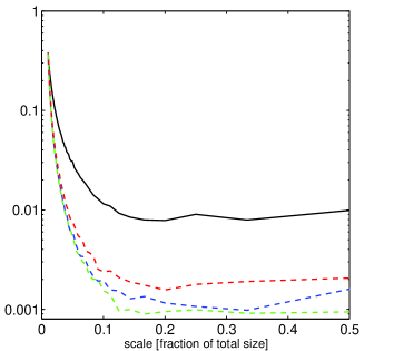
Figure 2: Energy momentum conservation of numerical simulations is shown. The lines represent the sum of the terms which has to vanish if energy (solid) respectively momentum (dashed) is conserved, divided by the sum of the absolute values of these terms. The abscissa indicates the wavelength of the perturbation as fraction of the size of the entire grid. (from [47]

The overall shape and amplitude of the unequal time correlators are quite similar to those found in the analytic large-$N$ approximation [145, 95, 45] (see Figs. 4 to 7). The main difference of the large-$N$ approximation is that there the field evolution, Eq. (121), is approximated by a linear equation. The non-linearities in the large-$N$ seeds, which are due solely to the energy momentum tensor being quadratic in the fields, are much weaker than in the texture model where the field evolution itself is non-linear. Therefore, decoherence which is a purely non-linear effect, is much weaker in the large-$N$ limit. This is actually the main difference between the two models as can be seen in Fig. 3. Otherwise the similarity of the results obtained by simulating the full non-linear problem and by considering the simplified linear limit is quite remarkable. The entire class of global $O(N)$ models behaves in this way, and potentially many other global defect models as well.

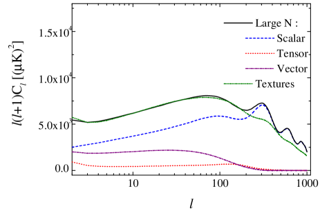
Figure 3: The $C_{\ell}$ power spectrum is shown for the large-$N$ limit (bold line) and for the texture model. The main difference is clearly that the large-$N$ curve shows some acoustic oscillations which are nearly entirely washed out in the texture case.

4.2 Cosmic strings

So far we discussed only theories with global defects. Yet in modern particle physics, local (gauge) symmetries play a much more important role than global symmetries. As we have seen in Chapter 2, strings are the only local defects which scale and which are therefore potential candidates to seed structure formation. Most research concentrates on local $U(1)$ theories, the best known cosmic strings. But also other models, even with non-abelian strings, have been considered (see e.g.  [136, 18]).

The main difference for the numerical treatment of local strings as compared to global defects is due to the existance of a gauge field which compensates the gradient energy of the field. All the energy is therefore concentrated in the tiny region of order the symmetry breaking scale $l_{M}\sim 1/M\sim 1/T_{c}$ where the scalar field leaves the vacuum manifold. Let us estimate how thin cosmic strings really are: COBE normalisation requires the phase transition to take place at the GUT scale, $T_{c}\sim 10^{16}$GeV. This corresponds to $l_{m}\sim 1/T_{c}\sim 10^{-30}$ cm. Clearly, a numerical simulation with a grid of not much more than $(512)^{3}$ cells which should simulate the entire Hubble volume, $\sim(10^{28}{\rm cm})^{3}$, cannot resolve this scale by more than $55$ orders of magnitude. Therefore, strings are approximated as infinitely thin, and it can be shown that they obey to a very good approximation the Nambu-Goto action of fundamental string theory [152]. Corrections are of the order of the string thickness devided by the string curvature scale, and therefore irrelevant for cosmology.

Furthermore, the string network needs to loose energy by gravitational radiation in order to scale. Hence, energy momentum conservation cannot be enforced for the defect field alone, leading to 14 UTCs insted of only five. As the interactions of cosmic strings are not known, one must also make ad hoc assumptions concerning the decay products. This choice has considerable impact on the results [26, 124].

We do not describe the numerical simulations to evolve cosmic strings. Detailed accounts of this problem can be found in the literature [152, 71, 106, 153]. Let us, nevertheless, point out the main problem. It is very difficult to simulate cosmic strings in expanding space, due to the large difference between the Hubble scale and the scale of small scale structure. Hence, it remains unclear up to date, whether string simulation in an expanding universe can capture enough of the small scale structure, the tiny wiggles and loops which develop due to the string self-interaction, to produce meaningful results. On the other hand, string simulations in flat space, do not satisfy energy momentum conservation of expanding space. To adress the small scale structure problem, most of the recent results in the literature, actually all except [4, 5, 7], use flat space simulations or semi-analytical methods to calculate the string UTC’s. It is not clear to us which procedure gives the best results, but since all the obtained CMB spectra disagree significantly with observations, this question has somehow lost its urgency.

As initial configuration of a string simulation, one usually lays down string segments according to the so called Vachaspati-Vilenkin algorithm. These are then evolved with the Nambu-Goto equation of motion. The physical problem of the ’decay product’ of cosmic strings is related to the numerical problem of small scale structure: Most string codes find that the network develops structure (wiggles, tiny loops) on the smallest scales which the simulation can resolve. The phyical scale of these small wiggles and loops is still unknown. It may even be, that the loops become smaller and smaller due to self-intersection, until their size is of the order of their thickness and they decay into elementary particles. This picture, which is in contrast to the decay into gravity waves, is avocated in Ref. [154]. There have also been several attempts to take into account these wiggles in semi-analytic models [121].

5 Result

5.1 The unequal time correlators

As explained in Chapter 3 to compute the observable CMB and matter, power spectra we need the unequal time correlators of the seed energy momentum tensor.

More precisely, for the scalar part we need the correlators

$$\langle\Phi_{s}(\mbox{\boldmath$k$},\tau)\Phi_{s}^{*}(\mbox{\boldmath$k$},\tau^{\prime})\rangle = \frac{1}{k^{4}\sqrt{\tau\tau^{\prime}}}C_{11}(z,r)~{},$$ (131)

$$\langle\Phi_{s}(\mbox{\boldmath$k$},\tau)\Psi_{s}^{*}(\mbox{\boldmath$k$},\tau^{\prime})\rangle = \frac{1}{k^{4}\sqrt{\tau\tau^{\prime}}}C_{12}(z,r)~{},$$ (132)

$$\langle\Psi_{s}(\mbox{\boldmath$k$},\tau)\Psi_{s}^{*}(\mbox{\boldmath$k$},\tau^{\prime})\rangle = \frac{1}{k^{4}\sqrt{\tau\tau^{\prime}}}C_{22}(z,r)~{},$$ (133)

as well as $C_{21}(z,r)=C^{*}_{12}(z,1/r)$. The functions $C_{ij}$ are analytic in $z^{2}$. The pre-factor $1/(k^{4}\sqrt{\tau\tau^{\prime}})$ comes from the fact that the correlation functions $\langle f_{\rho}f^{*}_{\rho}\rangle$, $k^{4}\langle f_{\pi}f^{*}_{\pi}\rangle$ and $k^{2}\langle f_{v}f^{*}_{v}\rangle$ have to be analytic and from dimensional considerations (see Ref. [45]).

The functions $C_{ij}$ are shown in Fig. 4. Panels (a) are obtained from numerical simulations. Panels (b) represent the same correlators for the large-$N$ limit of global $O(N)$-models (see [146, 95]).

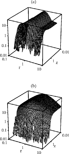
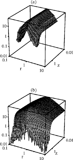
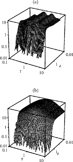
Figure 4: The two point correlation functions $C_{11}(z,r)=k^{4}\sqrt{\tau\tau^{\prime}}\langle\Phi_{s}(\mbox{\boldmath$k$},t)\Phi_{s}^{*}(\mbox{\boldmath$k$},\tau^{\prime})\rangle$ (left), $C_{22}(z,r)=k^{4}\sqrt{\tau\tau^{\prime}}\langle\Psi_{s}(\mbox{\boldmath$k$},\tau)\Psi_{s}^{*}(\mbox{\boldmath$k$},\tau^{\prime})\rangle$ (center) and $|C_{12}(z,r)|=k^{4}\sqrt{\tau\tau^{\prime}}|\langle\Phi_{s}(\mbox{\boldmath$k$},\tau)\Psi_{s}^{*}(\mbox{\boldmath$k$},\tau^{\prime})\rangle|$ (right). Panels (a) represent the result from numerical simulations of the texture model; panels (b) show the large-$N$ limit. For fixed $r$ the correlator is constant for $z<1$ and then decays. Note also the symmetry under $r\rightarrow 1/r$ for $C_{11}$ and $C_{22}$ which is lost for $C_{12}$ (from [47]).

In Fig. 5 we show $C_{ij}(z,r=1)$, and the ’constant’ of the Taylor expansion for $C_{ij}$ is given as a function of $r$, i.e., $C_{ij}(0,r)$.

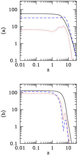
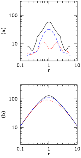
Figure 5: On the left the correlators $C_{ij}(z,1)$ are shown, while the right figure depicts $C_{ij}(0,r)$ with $r=\tau^{\prime}/\tau$. The solid, dashed and dotted lines represent $C_{22}~{},~{}C_{11}$ and $|C_{12}|$ respectively. Panels (a) are obtained from numerical simulations of the texture model and panels (b) show the large-$N$ limit. A striking difference is that the large-$N$ value for $|C_{12}|$ is relatively well approximated by the perfectly coherent result $\sqrt{|C_{11}C_{22}|}$ while the texture curve for $|C_{12}|$ lies nearly a factor 10 lower (from [47]).

Vector perturbations are induced by $\mbox{\boldmath$\Sigma$}^{(s)}$ which is seeded by $\mbox{\boldmath$w$}^{(v)}$. Transversality and dimensional arguments require the correlation function to be of the form

$$\langle w_{i}^{(v)}(\mbox{\boldmath$k$},t)w_{j}^{(v)*}(\mbox{\boldmath$k$},\tau^{\prime})\rangle=\sqrt{\tau\tau^{\prime}}(k^{2}\delta_{ij}-k_{i}k_{j})W(z,r)~{}.$$ (134)

Again, as a consequence of causality, the function $W$ is analytic in $z^{2}$ (see [45]). The functions $W(z,r)$, $W(z,1)$ and $W(0,r)$ are plotted in Fig. 6.

 

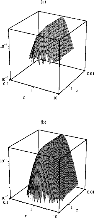
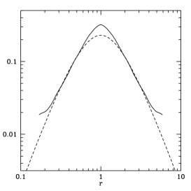
Figure 6: The vector correlator $W(z,r)$ is shown on the left. The texture simulations, panel (a), and the large-$N$ limit, panel (b), give very similar results, up to a slight difference in amplitude. On the right we see $W(z,1)$ (top) and $W(0,r)$ (bottom). The solid line represents the texture simulations and the dashed line is the large-$N$ result. The ‘wings’ visible in the lower texture curve are probably not due to a resolution problem but the beginning of oscillations (from [47]).

Symmetry, transversality and tracelessness, together with statistical isotropy require the tensor correlator to be of the form (see [45])

$$\langle\tau^{(\pi)}_{ij}(\tau)\tau^{(\pi)*}_{lm}(\tau^{\prime})\rangle=\frac{1}{\sqrt{\tau\tau^{\prime}}}T(z,r)[\delta_{il}\delta_{jm}+\delta_{im}\delta_{jl}$$ (135)

$$-\delta_{ij}\delta_{lm}+k^{-2}(\delta_{ij}k_{l}k_{m}+\delta_{lm}k_{i}k_{j}-\delta_{il}k_{j}k_{m}-\delta_{im}k_{l}k_{j}$$

$$-\delta_{jl}k_{i}k_{m}-\delta_{jm}k_{l}k_{i})+k^{-4}k_{i}k_{j}k_{l}k_{m}]~{}.$$

The functions $T(z,r)$ as well as $T(z,1)$ and $T(0,r)$ are shown in Fig. 7.

 

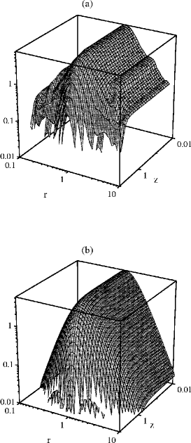
Figure 7: The tensor correlator $T(z,r)$ is shown on the left, the texture simulations in panel (a), and the large-$N$ limit in panel (b). On the right we see $T(z,1)$ (top) and $T(0,r)$ (bottom). The solid lines represent texture simulations and the dashed lines are the large-$N$ result. (from [47])

Expanding the unequal time correlators in terms of eigenfunctions and eigenvectors as explained in Chapter 3, one finds that ae expansion with a linear weight actually converges faster than one with a logarithmic weight. This is illustrated in Fig. 8 below.

 

Figure 8: The sum of the first few eigenfunctions of $T(x,x)$ is shown for two different weight functions, (a) logarithmic, $w=1/x$ and (b) linear, $w=1$. The first (long dashed), first and second (short dashed), first ten (dotted) and first thirty (solid) eigenfunctions are summed up. The open circles represent the full correlation function. Clearly, the eigenfunctions obtained by linear weighting converge much faster. Here we only show the equal time diagonal of the correlation matrix, but the same behavior is also found in the $C_{\ell}$ power spectrum which is sensitive to the full correlation matrix (from Re. [47]).

Figure 9: The size of the equal time contribution from the energy density (solid line) and the anisotropic stresses (left). Pressure, velocity and vorticity are of about the same size as the anisotropic stresses (right) (from Magueijo & Brandenberger [106]).

In Fig. 9 we also show the equal time correlators of the energy density and pressure, velocity and anisotropic stresses of local cosmic strings. It is interesting to note to which extent the spatial components of the energy momentum tensor are smaller than the energy density. In contrary to global defects, local strings provide a nearly non-relativistic source.

A source is called totally coherent [105, 49] if the unequal time correlation functions can be factorized. This means that only one eigenvector is relevant. A simple totally coherent approximation, which however misses some important characteristics of defect models, can be obtained by replacing the correlation matrix by the square root of the product of equal time correlators,

$$\langle{\cal S}_{i}(\tau){\cal S}_{j}^{*}(\tau^{\prime})\rangle\rightarrow\pm\sqrt{\langle|{\cal S}_{i}(\tau)|^{2}\rangle\langle|{\cal S}_{j}(\tau^{\prime})|^{2}\rangle}~{}.$$ (136)

This approximation is exact if the source evolution is linear. Then the different $k$ modes do not mix and the value of the source term at fixed $k$ at time $\tau$ is given by its value at initial time multiplied by some transfer function, ${\cal S}(\mbox{\boldmath$k$},\tau)=T(\mbox{\boldmath$k$},\tau,\tau_{in}){\cal S}(\mbox{\boldmath$k$},\tau_{in})$. In this situation, (136) becomes an equality and the model is perfectly coherent. Decoherence is due to the non-linearity of the source evolution which induces a ’sweeping’ of power from one scale into another. Different wave numbers $k$ do not evolve independently.

It is interesting to note that the perfectly coherent approximation (136) leaves open a choice of sign which has to be positive if $i=j$, but which is undetermined otherwise. According to Schwarz inequality the correlator $\langle{\cal S}_{i}(\tau){\cal S}_{j}^{*}(\tau^{\prime})\rangle$ is bounded by

$$\!\!\!\!-\sqrt{\langle|{\cal S}_{i}(\tau)|^{2}\rangle\langle|{\cal S}_{j}(\tau^{\prime})|^{2}\rangle}\leq\langle{\cal S}_{i}(\tau){\cal S}_{j}^{*}(\tau^{\prime})\rangle\leq\sqrt{\langle|{\cal S}_{i}(\tau)|^{2}\rangle\langle|{\cal S}_{j}(\tau^{\prime})|^{2}\rangle}.$$

Hence, for scales/variables for which the Greens function is not oscillating (e.g. Sachs Wolfe scales) the full result always lies between the ’anti-coherent’ (minus sign) and the coherent result. This behavior has been verified numerically [47].

The first evidence that acoustic peaks are suppressed in defect models has been obtained in the perfectly coherent approximation in Ref. [44]. In Fig. 10 we show the contributions to the $C_{\ell}$’s from more and more eigenvectors. A perfectly coherent model has only one non-zero eigenvalue.

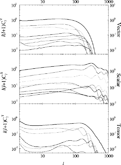
Figure 10: The scalar, vector and tensor contributions for the texture model of structure formation are shown. The dashed lines show the contributions from single eigenfunctions while the solid line represents the sum. Note that the single contributions to the scalar and tensor spectrum do show oscillations which are however washed out in the sum. (Vector perturbations do not obey a wave equation and thus do not show oscillations.)

A comparison of the full result with the totally coherent approximation is presented in Fig. 11.

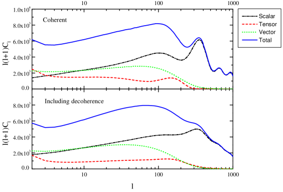
Figure 11: The $C_{\ell}$ power spectrum for the texture scenario is shown in the perfectly coherent approximation (top panel) and in the full eigenfunction expansion. Even in the coherent approximation, the acoustic peaks are not higher than the Sachs Wolfe plateau. Decoherence just washes out the structure but does not significantly damp the peaks.

There one sees that decoherence does smear out the oscillations present in the fully coherent approximation, and does somewhat damp the amplitude. Decoherence thus prevents the appearance of a series of acoustic peaks. The absence of power on the angular scale of the peaks, however, is not a consequence of decoherence. Is mainly due to the anisotropic stresses of the source, which lead to perturbations in the geometry inducing large scale $C_{\ell}$’s (Sachs Wolfe), but not to density fluctuations, which are responsible for the acoustic peaks. Large anisotropic stresses are also at the origin of vector and tensor fluctuations which contribute more than 50% on large scales. These results were first computed fully in Ref. [117] and followed by a parameter study in Ref [47]. Thy are in agreement with Ref. [44] but disagree strongly with Ref. [28].

In the real universe, perfect scaling of the seed correlation functions is broken by the radiation–matter transition, which takes place at the time of matter and radiation equality, $\tau_{eq}\simeq$ $20h^{-2}\Omega_{m}^{-1/2}$Mpc. The time $\tau_{eq}$ is an additional scale which enters the problem and influences the seed correlators. Only in a purely radiation or matter dominated universe are the correlators strictly scale invariant. This means actually that the $k$ dependence of the correlators $C$, $W$ and $T$ cannot really be cast into a dependence on $x$ and $x^{\prime}$, but that these functions depend on $\tau,\tau^{\prime}$ and $k$ in a more complicated way. In principle, one thus has to calculate and diagonalize the seed correlators for each wave number $k$ separately and the huge gain of dynamical range is lost as soon as scaling is lost.

In the actual case at hand, however, the deviation from scaling is weak, and most of the scales of interest for structure formation (especially those which are still in the linear regime) enter the horizon only in the matter dominated era. The behavior of the correlators in the radiation dominated era is of minor importance. To solve the problem, one can calculate the eigenvalues and eigenfunctions twice, in a pure radiation and in a pure matter universe and interpolate the source term from the radiation to the matter epoch. Denoting by $\lambda_{m},v_{m}$ and $\lambda_{r},v_{r}$ a given pair of eigenvalue and eigenvector in a matter and radiation universe respectively, we choose as our deterministic source function

$$v(\tau) = y(\tau)\sqrt{\lambda_{r}}v_{r}(k\tau)+(1-y(\tau))\sqrt{\lambda_{m}}v_{m}(k\tau)$$ (137)

with, e.g.,

$$y(\tau) = \frac{\tau_{eq}}{\tau+\tau_{eq}}~{}~{}\mbox{ or }~{}~{}~{}y(\tau)=\exp(-\tau/\tau_{eq})~{},$$ (138)

or some other suitable interpolation function. The effect of the radiation dominated early state of the universe is relatively unimportant for the scales of interest for CMB anisotropies and linear gravitational clustering The difference between the pure matter era result and the interpolation is very small [47]. This seems to be quite different for cosmic strings where the fluctuations in the radiation era are about twice as large as those in the matter era [132]. The radiation dominated era has, however, little effect on the key feature of CMB anisotropies from topological defects; namely the absence of acoustic peaks.

In models with cosmological constant, there is actually a second break of scale invariance at the matter–$\Lambda$ transition. There one can proceed in the same way as outlined above. Since defects cease to scale and disappear rapidly in an exponentially expanding universe, the eigenvalues for the $\Lambda$ dominated universe all vanish.

In Fig. 12 we show the CMB power spectrum from cosmic strings. Predictions from different research groups working on the subject [5, 7, 26, 105, 124, 121] agree only partially. Contrary to global defects models, there seems to be a broad peak at rather high $\ell\sim 400$ to $500$. The height of the peak is very much a matter of debate. In some work it is completely absent [5], while in other it is quite high [26, 121]. We can maybe understand this difference between global and local defects as being due to the larger difference between the source functions in the radiation and matter dominated era: For the global $O(N)$ defects, the ratio between the sources in the two epochs is about $1.2$, while for strings it is rather in the vicinity of $4$ [160]. This difference can explain the more prominent peak at high $\ell$ for cosmic strings. An additional intriguing difference to global defect is the strong domination of the energy density over the rest of the energy momentum tensor (see Fig. 9). The dependence of the spectrum on the equation of state of the decay product, $p_{X}=w_{X}\rho_{X}$ is remarkable.

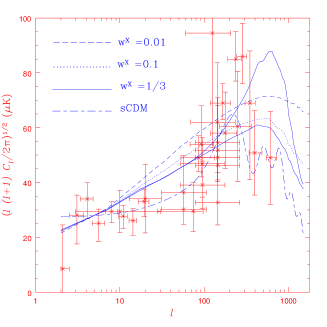
Figure 12: The angular CMB power spectrum of cosmic strings, from a simulation by Contaldi, Hindmarsh and Magueijo [26]. The figure shows the result for strings decaying into a fluid obeying the equation of state $p=w\rho$. with $w=1/3,~{}0.1,~{}0.01$ respectively. The old data overlaid to the graph is to be ignored.

A feature which the two classes of defects have in common is decoherence which smears out all secondary peaks. Furthermore, cosmic strings seem to suffer as well from insufficient power on large scales in the dark matter. The clear sequence of acoustic peaks recently observed [110, 66, 97] rules out any seeds with strongly non-linear evolution, such as $O(N)$ (with low $N$), both for global and local gauge theories, as well as any other non-linear mechanism for seeding cosmic perturbations!

5.2 non-Gaussianity

An interesting difference between structure formation with topological defects and inflationary models is also that the latter have generically Gaussian perturbations while the former don’t. Even if the defect energy momentum tensor would be Gaussian initially, non-linear evolution induces non-Gaussianities. (Recently, however, a model leading to Gaussian fluctuations from cosmic defects has been investigated [6].)

Even if the fields themselves would be Gaussian (which they are not), the energy momentum tensor, which is quadratic in the fields, would obey a $\chi^{2}$-distribution. But the $\sigma$-model condition $\sum_{i=1}^{N}(\beta_{i})^{2}=1$ cannot be satisfied if the fields $\beta_{i}$ are Gaussian random variables. In the large $N$ model, the $O(N)$-model in the limit $N\rightarrow\infty$, the energy momentum tensor is a infinite sum of variables $\partial_{\mu}\beta_{i}\partial_{\nu}\beta_{i}$ which all obey the same distribution. This large $N$ model is nearly Gaussian as a consequence of the central limit theorem. The fact that the variables $\beta_{i}$ have to satisfay the normalization condition however implies that the variables $\partial_{\mu}\beta_{i}\partial_{\nu}\beta_{i}$ are not statistically independent.

Clearly, $O(N)$-models with $N>4$ components do not lead to topological defects in $3$-dimensional space, but in the large $N$-limit the equations of motion can be solved analytically and, as we have already seen, the model is very useful to study certain features of $O(N)$ defects. The fact that non-Gaussianity becomes weaker as $N$ becomes larger, indicates that cosmic strings are probably the most non-Gaussian defects and textures are the least non-Gaussian.

For defects to be non-Gaussian, means that their energy momentum tensor does not obey Gaussian statistics. Therefore certain reduced higher oder moments do not vanish. It is not evident how to find the best observable to locate the non-Gaussianity. Some suggestions for variables which might be useful in the case of defects have been proposed in Refs. [54, 59]. Furthermore, a given observational variable like,e.g. , the integrated Sachs-Wolfe effect, may be the sum of many non-Gaussian but equally distributed contributions and hence be very closely Gaussian due to the central limit theorem.

Unfortunately, it is not known how strong non Gaussian features are in the CMB or in the dark matter distribution of topological defect models. It is also not clear on which scales they are strongest. Due to the arguments indicated above, we expect cosmic strings to be most non-Gaussian. A well distinguished non-Gaussian feature in CMB anisotropies from cosmic strings is the Kaiser-Stebbins effect [91]. This is a disconinuity in the CMB temperature due to a moving string between the observer and the CMB. Even though this effect is easily obtained analytically for a straight cosmic string, it is difficult to get a handle on it in a string network of many bent and twisted strings which also contain small scale structure. One expects the Kaiser-Stebbins effect to be relevant for the anisotropies on about arc-minute scale.

Old partial results on non-Gaussianity from numerical simulations (see e.g. . [118, 51]) are probably strongly affected by finite size effects and not very reliable. On the other hand, with the more successful method to compute power spectra just by determining the unequal-time two point distribution of the defects, one loses all information about higher order correlations and thus about non-Gaussianity. Since the known defects are such a bad fit to the present CMB data, nobody has been sufficiently motivated to study and solve the difficult problem of the non-Gaussianity which defects may induce in the CMB anisotropies or in the matter distribution. A semi-analytic study of the bi-spectrum, the third moment of CMB anisotropies for cosmic strings can be found in Ref. [59].

We know that also non-linear Newtonian clustering induces non-Gaussianities. The reduced $n$-point functions in the matter distribution due to non-linear clustering scale like $D^{2n-2}$, where $D$ is the matter density perturbation amplitude (see e.g.  [58]). In contrary, a non-Gaussianity already present at the linear level simply scales like $D^{n}$ in the $n$-point function [43]. Therefore, initial non-Gaussianities, like those of defects are best detected on large scales, where non-linearities are negligible since $D\ll 1$. On small scales, where non-linearities are important, the non-Gaussianity from Newtonian clustering is stronger than the one form the initial conditions. Therefore, the fact that non-linearities in the observed galaxy distribution closely follow the behavior expected from Newtonian clustering, does not constrain topological defects very strongly.

5.3 CMB anisotropies and polarization

The $C_{\ell}$’s for the global texture model are shown in Fig. 11, bottom panel.

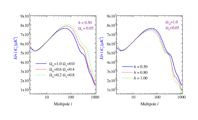
Figure 13: The $C_{\ell}$ power spectrum is shown for different values of cosmological parameters. In the right panel we choose $\Omega_{\Lambda}=0$, $\Omega_{CDM}=0.95$, $\Omega_{b}=0.05$ and vary $h$. In the left panel we fix $h=0.5$, $\Omega_{b}=0.05$ and vary $\Omega_{\Lambda}$. We only consider spatially flat universes, $\Omega_{0}=1$.

Vector and tensor modes are of the same order as the scalar component at COBE-scales. For the ’standard’ texture model one has $C_{10}^{(S)}:C_{10}^{(V)}:C_{10}^{(T)}\sim 0.9:1.0:0.3$. These results were found numerically and by analytical arguments in Refs. [117, 5, 2, 47] and [45]. Due to tensor and vector contributions, even assuming perfect coherence (see Fig. 11, top panel), the total power spectrum does not increase from large to small scales. Decoherence leads to smoothing of oscillations in the power spectrum at small scales and the final spectrum has a smooth shape with a broad, low isocurvature ’hump’ at $\ell\sim 100$ and a small residual of the first acoustic peak at $\ell\sim 350$. There is no structure of peaks at small scales. The power spectrum is well fitted by the following fourth-order polynomial in $x=\log\ell$:

$${\ell(\ell+1)C_{\ell}\over 110C_{10}}=1.5-2.6x+3.3x^{2}-1.4x^{3}+0.17x^{4}~{}.$$ (139)

The effect of decoherence is less important for the large-$N$ model, where oscillations and peaks are still visible (see Fig 3, bottom panel). As argued before, this is due to the fact that the non-linearity of the large-$N$ limit is only in the quadratic energy momentum tensor. Since decoherence is inherently due to non-linearities, we expect it to be stronger for lower values of $N$.

In Fig. 13 we plot the global texture $C_{\ell}$ power spectrum for different choices of cosmological parameters. The variation of parameters leads to similar effects like in the inflationary case, but with smaller amplitude. At small scales ($\ell\geq 200$), the $C_{\ell}$’s tend to decrease with increasing $H_{0}$ and they increase when a cosmological constant $\Omega_{\Lambda}=1-\Omega_{m}$ is introduced. Nonetheless, the amplitude of the anisotropy power spectrum at high $\ell$s remains in all cases on the same level like the one at low $\ell$s, without showing the substantial peak found in inflationary models and in the data. The absence of acoustic peaks is a stable prediction of global $O(N)$ models. The models are normalized to the full CMB data set, which leads to slightly larger values of the normalization parameter than pure COBE normalization. An avarage value for different choices of cosmological parameters is $\epsilon=4\pi G\eta^{2}\sim 1.6$

We compare the texture results with the three best current experimental data sets from Boomerang-98 [110], Maxima [97] and DASI [66]. We take in to account the calibration uncertainty of $10\%$ for Boomerang and of $5\%$ for Maxima and DASI. We also include the COBE dataset using Lloyd Knox’s RADPack packages [166].

No matter how precisely an experiment will measure the CMB sky, the result will be always affected by the intrinsic statistics of the perturbations, i.e. the cosmic variance. In the recovery of the power spectra of the above experiments, the temperature distribution is often assumed to be Gaussian. Deviation from Gaussianity could lead to an enhancement of the cosmic variance, which can be as large as a factor of $7$ (see [103]). Inevitably therefore, the quoted error-bars in the CMB power spectrum could be in principle underestimated by the assumption of the Gaussian statistic. This effect is, however only relevant for relatively low $\ell$s. Furthermore, preliminarly statistical analysis of the Maxima map [161] have found no-evidence for non-Gaussianities. Keeping this caveat in mind, but missing a more precise alternative, we indicate the minimal, Gaussian error calculated according to the published data. The numerical seeds taken from [47] are assumed to be about 10% accurate. In Fig. 14 we plot the Boomerang and DASI data together with the theoretical predictions for a texture model with $h=0.65$,$\Omega_{\Lambda}=0.625$, $\Omega_{cdm}=0.315$ and $\Omega_{b}=0.06$, and the corresponding inflationary model with $n_{s}=0.98$ which gives a best fit to the data. All of the experiments detect a very clear first peak at $\ell\approx 200$ which is incompatible with all $O(N)$ models [44, 117, 128, 47] as well as with the cosmic string results [26, 121, 124] In Table 1, we report the $\chi^{2}$ values from a comparison of the CDM-texture model with each experiment, separately. As we can see, while in reasonable agreement with the large angular scale data from the COBE experiment, the new data at intermediate and small angular scales from BOOMERanG, DASI and MAXIMA rule out the model with high significance.

In addition, the data shows indications of a series of peaks pointing to coherent acoustic oscillations. If the evidence for this peak sequence strenghtens once new data becomes available, it will provide strong evidence against non-linear mechanisms for the generation of perturbations. Furthermore, it will enable us to place stringent limits on the relative amounts of isocurvature and adiabatic contributions to the perturbations. We present a more general discussion in the next chapter.

Experiment	Data Points	$\chi^{2}$
COBE	24	28
COBE+B98	43	317
B98	19	221
COBE+MAXIMA	36	119
MAXIMA	12	32
COBE+DASI	33	246
DASI	9	75

Table 1: Topological defects versus CMB data. While in reasonable agreement with the COBE data, the power spectrum inferred from textures is in strong disagreement with the present intermediate and small angular scale observations. The BOOMEranG data alone, in particular, rule out the model at extremely high significance.

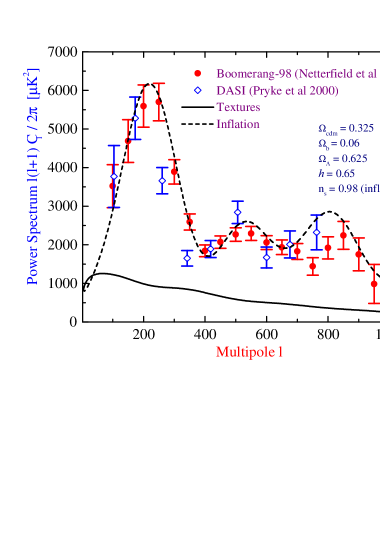
Figure 14: The $C_{\ell}$ spectrum obtained in the standard texture model is compared with the recent BOOMERANG and DASI data. A standard inflationary model, which gives a much better fit to the data, is also plotted.

Finally, we compare $E$- and $B$-type polarisation induced by defects with the result of an inflationary model with equal amplitude of scalar and tensor temperature fluctuations in Fig. 15 . Due to the amount of vector perturbations present, it is not surprising that $B$-type polarization has significantly higher amplitude for defects. Furthermore, the isocurvature shift of the ’acoustic peaks’ and decoherence are also visible in the polarisation signal.

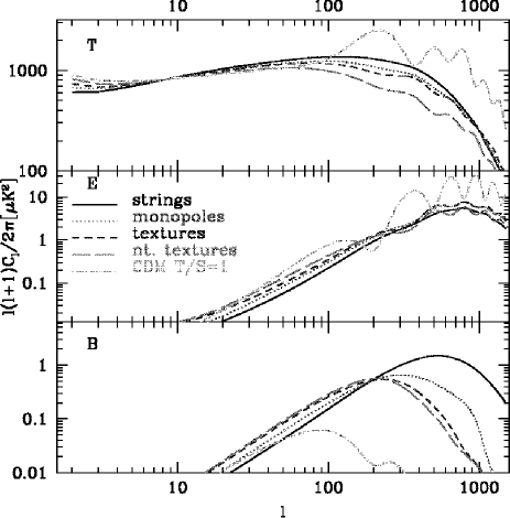
Figure 15: Power spectra of temperature (T), electric type polarization (E) and magnetic type polarization (B) for global strings, monopoles, textures and an $O(N)$ scalar field with $N>4$ are shown. For comparison, also the corresponding spectra in a standard CDM model with $T/S=1$ (which maximizes the B component) is plotted. All defect models predict a much larger component of B polarization on small angular scales (from Seljak, Pen and Turok [128]).

5.4 Matter power spectra

The first serious attempts to compute the matter distribution in scenarios with topological defects were done for cosmic strings [108]. But due to the problems inherent in cosmic string simulations, the accuracy of these results may well be less that a factor of two or three.

The situation is different for global defects. There, the first accurate matter spectra have been computed in Ref. [117]. This work, which underestimated the vector and tensor contribution to CMB anisotropies, still had the wrong normalization. This was corrected later in [51, 117, 47]. For a COBE mormalized global texture model, the total mass fluctuation $\sigma_{R}$ in a ball of radius $R=8h^{-1}$Mpc, is about $\sigma_{8}=(0.44\pm 0.07)h$ (the error coming from the CMB normalization) in a flat universe without cosmological constant (see Refs. [117, 47]. From the observed cluster abundance, one infers $\sigma_{8}=(0.50\pm 0.04)\Omega^{-0.5}$ [52] and $\sigma_{8}=0.59^{+0.21}_{-0.16}$ [99]. These results, which are obtained with the Press-Schechter formula, assume Gaussian statistics. We thus have to take them with a grain of salt, since we do not know how non-Gaussian fluctuations on cluster scales are in the texture model. According to Ref. [57], the Hubble constant lies in the interval $h\simeq 0.73\pm 0.06\pm 0.08$. Hence, in a flat CDM cosmology, taking into account the uncertainty of the Hubble constant, the texture scenario predicts a reasonably consistent value of $\sigma_{8}$.

However, as discussed in Refs. [2], [117] and [47], unbiased global texture models are unable to reproduce the power of galaxy clustering at very large scales, $\stackrel{{\scriptstyle>}}{{\sim}}20h^{-1}$ Mpc. In order to quantify this discrepancy we compare the prediction of the linear matter power spectrum with the decorrelated linear power spectrum of the PSCz survey from [67] in Fig. 17. Clearly, the textures model without a cosmological constant provides a bad fit to the large scale data. Including a cosmological constant improves the agreement between the shape of the theoretical spectrum and the data. However, the required bias is too high, $b\sim 6$ and the model fails to match the observed value of $\sigma_{8}$. We further test this discrepancy by comparing the theoretical predictions with the results from a wide number of infrared (Refs. [56],[142]) and optically-selected (Refs. [29], [102]) galaxy redshift surveys, and with the real-space power spectrum inferred from the APM photometric sample (Ref. [10]). All the results are in rough agreement with the PSCz comparison: For $h=0.5$ and $\Omega_{\Lambda}=0.8$ the shape of the texture power spectrum fits the data well, but the bias is very high. The only exception is the APM data, the shape of which cannot be fitted with the texture spectrum. In Table 2 we report for each survey the best cosmological parameter $(h,\Omega_{\Lambda})$ within the limited ones which have been analysed, and the best value of the bias parameter obtained by $\chi^{2}$-minimization. We also indicate the value of $\chi^{2}$ (not divided by the number of data points) and the number of data points. The bias parameter strongly depends on the data considered. This is not surprising, since also the catalogs are biased relative to each other. A more detailed discussion of this analysis is found in Ref. [47].

The power spectra for the large-$N$ limit and for the coherent approximation are typically a factor 2 to 3 higher (see Fig. 16), and the biasing problem is alleviated for these cases. For $\Omega_{\Lambda}=0$ we find $\sigma_{8}=0.57h$ for the large-$N$ limit and $\sigma_{8}=0.94h$ for the coherent approximation. This is no surprise since only one source function, $\Psi_{s}$, the analog of the Newtonian potential, seeds dark matter fluctuations and thus coherence always enhances the unequal time correlator. The dark matter Greens function is not oscillating, so this enhancement translates directly into the power spectrum.

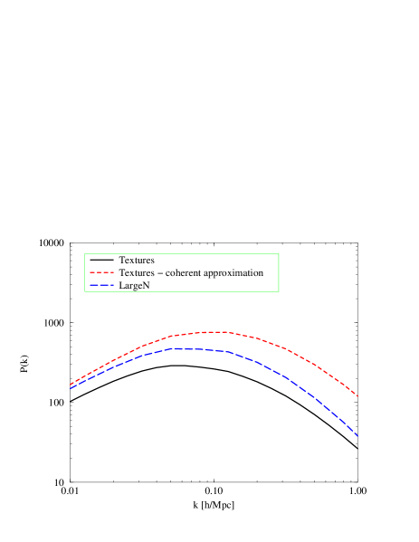
Figure 16: The dark matter power spectrum for the texture model (solid line) is compared with the coherent approximation (short dashed) and the large-$N$ limit (long dashed). The spectra are COBE normalized and the cosmological parameters are $\Omega_{\Lambda}=0~{},~{}h=0.5$.

Models which are anti-coherent in the sense defined in Section IID reduce power on Sachs-Wolfe scales and enhance the power in the dark matter. Anti-coherent scaling seeds are thus the most promising candidates which may cure some of the problems of global $O(N)$ models.

The analysis described here does not take into account the effects of non-linearities and redshift distortions. Redshift distortions in the texture case should be less important than in the inflationary case since the peculiar velocities are rather low (see next paragraph). Non-linearities typically set in at $k\geq 0.5h$Mpc^-1 and should not have a big effect on our main conclusions which come from much larger scales. Inclusion of these corrections will result in more small-scale power and in a broadening of the spectra, which even enhances the conflict between models and data. Furthermore, variations of other cosmological parameters, like the addition of massive neutrinos, hot dark matter, which are not considered here, will result in a change of the spectrum on small scales but will not resolve the discrepancy at large scales.

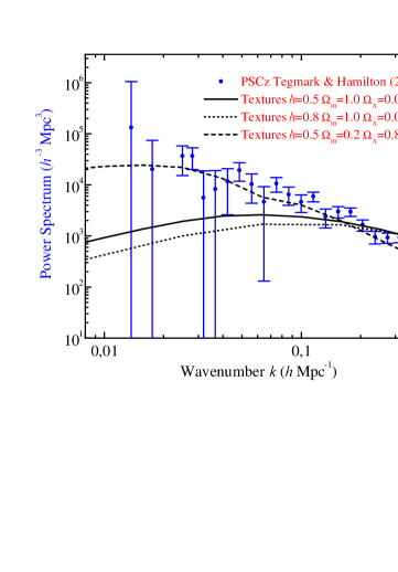
Figure 17: The matter Power spectrum: comparison between the PSCz data and theory.

Catalog	$h$	$\Omega_{\Lambda}$	Best fit bias $b$	$\chi^{2}$	Data points
CfA2-SSRS2 101 Mpc	0.5	0.8	9.5	4	24
CfA2-SSRS2 130 Mpc	0.5	0.8	11.1	4	19
LCRS	0.5	0.4	3.7	33	19
IRAS	0.5	0.8	6.3	9	11
IRAS 1.2 Jy	0.5	0.8	6.7	28	29
APM	0.5	0.0	3.3	1350	29
QDOT	0.5	0.8	7.3	14	19

Table 2: Analysis of the matter power spectrum. In the first column the catalog is indicated. Cols. 2 and 3 specify the model parameters. In cols. 4 and 5 we give the bias parameter inferred by $\chi^{2}$ minimization as well as the value of $\chi^{2}$. Col. 6 shows the number of ’independent’ data points assumed in the analysis.

5.5 Bulk velocities

To confirm the missing power on 20 to 100$h^{-1}$Mpc, we also consider the velocity power spectrum which is not plagued by the biasing problems of the galaxy distribution. The assumption that galaxies are fair tracers of the velocity field seems to us much better justified, than to assume that they are fair tracers of the mass density. We therefore test the global texture model against bulk velocity data (see also [47]). We use the data by Ref. [36] which gives the bulk flow

$$\sigma^{2}_{v}(R)={H_{0}^{2}\Omega_{m}^{1.2}\over{2\pi^{2}}}\int P(k)W(kR)dk~{},$$ (140)

in spheres of radii $R=10$ to $60h^{-1}$Mpc. These data are derived after reconstructing the $3-$dimensional velocity field with the POTENT method (see [36] and references therein).

As shown in Table 3, the COBE normalized texture model predicts too low velocities on large scales when compared with POTENT results. More recent measurements of the bulk flow lead to somewhat lower estimates like $\sigma_{v}(R)\sim(230\pm 90)$ at $R=60h^{-1}$Mpc (see Ref. [63]), but a discrepancy of about a factor of $2$ in the best case remains. Including a cosmological constant helps at large scales, but decreases the velocities on small scales. Similar results are obtained in models with cosmic strings. There, however, details depend on assumption about the fluid into which string loops decay. For loops decaying into radiation, models with cosmic strings have even less power on $50h^{-1}$Mpc.

R	$\sigma_{v}$ (R)	$\Delta_{v}$	$h=0.5$	$h=1.0$	$\Omega_{\Lambda}=0.8$
10	494	170	145	205	86
20	475	160	100	134	78
30	413	150	80	98	70
40	369	150	67	78	65
50	325	140	57	65	61
60	300	140	50	56	57

Table 3: Bulk velocities: Observational data from [36] and theoretical predictions. $\Delta_{v}$ estimates the observational uncertainty. The uncertainties on the theoretical predictions are around $\sim 30\%$. The models $\Omega_{\Lambda}=0$ with $h=0.5$ and $h=1$ as well as $\Omega_{\Lambda}=0.8,~{}h=0.5$ are given.

This comparison of models with data shows that $U(1)$ cosmic strings and global $O(N)$ models are clearly ruled out by present large scale structure data. In the next chapter we shall study whether generalizations or mixed models may survive.

6 Generalizations

So far we have studied some specific models of topological defects and we have found that they cannot reproduce the observed large scale structure of the universe. Even if they basically lead to a Harrison–Zel’dovich spectrum on large scales, the ’details’ just do not fit. The isocurvature nature of the induced perturbations together with the high amplitude tensor and especially vector contributions, lead to relatively high amplitude of fluctuations on very large scales. Therefore, the COBE–normalized acoustic ’peaks’ and the dark matter power spectrum typically are too low. In addition, decoherence smears out the anyway too low secondary peaks in the CMB anisotropy spectrum.

In this chapter we first study the question whether this feature is generic or just happens to occur in the specific models which we have analyzed in the preceding chapters. Then we want to investigate whether mixed models with inflationary perturbations and a defect component might fit the data better than pure inflationary perturbations.

6.1 Generic properties of the unequal time correlation functions

We start by deriving some generic properties of power spectra induced by topological defects. As we have seen in Chapter 2, the resulting perturbation power spectra are fully determined by the un-equal time correlators of the defect energy momentum tensor.

The main properties which we shall use to describe the defect correlators are causality, statistical homogeneity and isotropy and scaling. Since the nature of the defects resulting as a ’topological relicts’ from a phase transition does not enter directly in this analysis, we speak of ’scaling causal seeds’, seeds denoting any non-uniformly distributed form of energy which provide a perturbation to the homogeneous background fluid. In first order perturbation theory they evolve according to the unperturbed (in general non-linear) equations of motion. For simplicity, we assume the seeds to be coupled to the cosmic fluid only via gravity. A counter example to this are the $U(1)$ cosmic strings discussed before. As we have seen, the string CMB anisotropy power spectrum, especially the height of the acoustic peak, depends very sensitively on the details of the coupling of string seeds to matter [26, 124]. For uncoupled seeds the energy momentum tensor is covariantly conserved. To determine power spectra or other expectation values which are quadratic in the cosmic perturbations, we just need to know the unequal time correlation functions of the seed energy momentum tensor [45, 47],

$$\langle\Theta_{\mu\nu}(\mbox{\boldmath$k$},\tau)\Theta^{*}_{\sigma\rho}(\mbox{\boldmath$k$}^{\prime},\tau^{\prime})\rangle=M^{4}\widehat{C}_{\mu\nu\sigma\rho}(\mbox{\boldmath$k$},\tau,\tau^{\prime})\delta(\mbox{\boldmath$k$}-\mbox{\boldmath$k$}^{\prime})~{},$$ (141)

where $M$ is a typical energy scale of the seeds (e.g. the symmetry breaking scale for topological defects), which determines the overall perturbation amplitude. Here we define Fourier transforms with the normalization

$$\hat{f}({\bf k}) = {1\over\sqrt{V}}\int d^{3}xf({\bf x})\exp(i{\bf kx})~{};$$ (142)

$$f({\bf x}) = {\sqrt{V}\over(2\pi)^{3}}\int d^{3}k\hat{f}({\bf k})\exp(-i{\bf kx})~{}.$$ (143)

Seeds are causal, if

$$C_{\mu\nu\sigma\rho}({\bf x},\tau,\tau^{\prime})\equiv{1\over M^{4}}\langle\Theta_{\mu\nu}(\mbox{\boldmath$y$},\tau)\Theta^{*}_{\sigma\rho}(\mbox{\boldmath$y$}+\mbox{\boldmath$x$},\tau^{\prime})\rangle$$

vanishes for $|{\bf x}|>\tau+\tau^{\prime}$; and they are scaling, if $\widehat{C}$ depends on no other dimensional parameter than $k$, $\tau$ and $\tau^{\prime}$. From scaling we conclude that for purely dimensional reasons, we can write the correlations functions in the form

$$\widehat{C}_{\mu\nu\lambda\rho}({\bf k},\tau,\tau^{\prime})={1\over\sqrt{\tau\tau^{\prime}}}F_{\mu\nu\lambda\rho}(\sqrt{\tau\tau^{\prime}}\cdot{\bf k},\tau^{\prime}/\tau)~{},$$ (144)

where $F_{\mu\nu\lambda\rho}$ is a dimensionless function of the four variables $z_{i}\equiv\sqrt{\tau^{\prime}\tau}k_{i}$ and $r\equiv\tau^{\prime}/\tau$, which is analytic in $z_{i}$.

We also require the seed to decay inside the horizon, which implies

$$\lim_{{k\tau\rightarrow\infty}}\widehat{C}_{\mu\nu\lambda\rho}({\bf k},\tau,\tau^{\prime})=\lim_{{k\tau^{\prime}\rightarrow\infty}}\widehat{C}_{\mu\nu\lambda\rho}({\bf k},\tau,\tau^{\prime})=0~{}.$$ (145)

Furthermore, since the seeds interact with the cosmic fluid only gravitationally, $\Theta$ satisfies covariant energy momentum conservation,

$$\Theta^{\mu\nu}_{;\nu}=0~{}.$$ (146)

With the help of these four equations, we can, for example, express the temporal components, $\Theta_{0\mu}$ in terms of the spatial ones, $\Theta_{ij}$. The seed correlations are thus fully determined by the spatial correlation functions $\widehat{C}_{ijlm}$. Statistical isotropy, scaling and symmetry in $i,j$ and $l,m$ as well as under the transformation $i,j;k;\tau\rightarrow l,m;-k;\tau^{\prime}$ require the following form for the spatial correlation functions:

$$\widehat{C}_{ijlm}({\bf k},\tau,\tau^{\prime})=$$ (147)

$${1\over\sqrt{\tau\tau^{\prime}}}[z_{i}z_{j}z_{l}z_{m}F_{1}(z^{2},r)+$$

$$(z_{i}z_{l}\delta_{jm}+z_{i}z_{m}\delta_{jl}+z_{j}z_{l}\delta_{im}+z_{j}z_{m}\delta_{il})F_{2}(z^{2},r)+$$

$$z_{i}z_{j}\delta_{lm}F_{3}(z^{2},r)/r+z_{l}z_{m}\delta_{ij}F_{3}(z^{2},1/r)r+$$

$$+\delta_{ij}\delta_{lm}F_{4}(z^{2},r)+(\delta_{il}\delta_{jm}+\delta_{im}\delta_{jl})F_{5}(z^{2},r)]~{},$$

where the functions $F_{a}$ are analytic in $z^{2}\equiv\tau\tau^{\prime}k^{2}$, and for $a\neq 3$ they are invariant under the transformation $r\rightarrow 1/r$, $F_{a}(z^{2},r)=F_{a}(z^{2},1/r)$. The positivity of the power spectra $\widehat{C}_{ijij}({\bf k},\tau,\tau)=\langle|\Theta_{ij}|^{2}\rangle\geq 0$ leads to a series of positivity conditions for the functions $F_{a}$:

$$0 \leq F_{5}(z^{2},1)~{},$$ (148)

$$0 \leq F_{4}(z^{2},1)+2F_{5}(z^{2},1)~{},$$ (149)

$$0 \leq z^{2}F_{2}(z^{2},1)+F_{5}(z^{2},1)~{},$$ (150)

$$0 \leq z^{4}F_{1}(z^{2},1)+4z^{2}F_{2}(z^{2},1)+3F_{5}(z^{2},1)~{},$$ (151)

$$0 \leq z^{4}F_{1}(z^{2},1)+2z^{2}(F_{3}(z^{2},1)+2F_{2}(z^{2},1))$$ (152)

$$+F_{4}(z^{2},1)+2F_{5}(z^{2},1)~{}.$$

Since $\widehat{C}_{ijlm}$ is the Fourier transform of a real function,

$$\widehat{C}_{ijlm}({\bf k},\tau,\tau^{\prime})^{*}=\widehat{C}_{ijlm}(-{\bf k},\tau,\tau^{\prime})~{}.$$ (153)

Hence the ansatz (147) implies that the functions $F_{a}(z^{2},r)$ are real. Furthermore, decay inside the horizon (condition (145)) yields

$$\lim_{z^{2}r\rightarrow\infty}F_{a}(z^{2},r)=\lim_{z^{2}/r\rightarrow\infty}F_{a}(z^{2},r)=0~{}.$$ (154)

In addition, analyticity implies that the functions $F_{a}$ do not diverge in the limit $z\rightarrow 0$, thus

$$\lim_{z\rightarrow 0}F_{a}(z^{2},r)=A_{a}(r)$$

with

$$A_{a}(r)=A_{a}(1/r)~{}\mbox{ for all }a\neq 3~{}.$$

As an example, we show some of these functions in the large $N$ limit of global scalar field seeds (see Chapter 4). In Figs. 1 and 2 we present the functions $F_{5}(z^{2},r)$ and $F_{2}(z^{2},r)$.

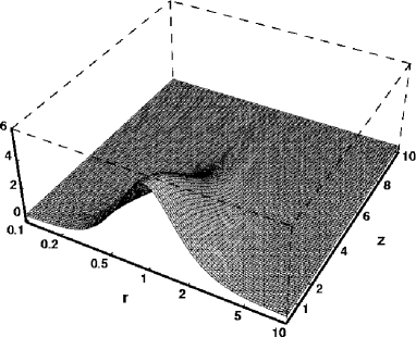
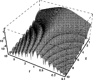
Figure 18: The function $F_{5}(z,r)$, linear (left) and $|F_{5}(z,r)|$ logarithmic are shown. Because of their small amplitude, the oscillations are invisible in the linear plot. To show the symmetry $r\rightarrow 1/r$, the $r$-axis is chosen logarithmic in both plots.

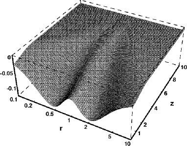
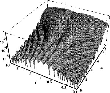
Figure 19: The same as Fig. 18 for the function $F_{2}(z,r)$.

The symmetry under the transition $r\rightarrow 1/r$ is clearly visible. Also the conditions that $F_{a}\rightarrow 0$ if either $z\rightarrow\infty$ or $r\rightarrow 0$ or $r\rightarrow\infty$ which follows from Eq. (154) is evidently satisfied. For fixed $z$ the functions oscillate with a frequency which grows with $z$. Since the amplitude decays rapidly, these oscillations are only visible in the log-plots. The correlations always decay like power laws, never exponentially.

The equal time correlation functions, $F_{1}(z^{2},1)$ to $F_{5}(z^{2},1)$ are plotted in Fig. 20 left. On the right hand side we show $A_{a}(r)$.

 

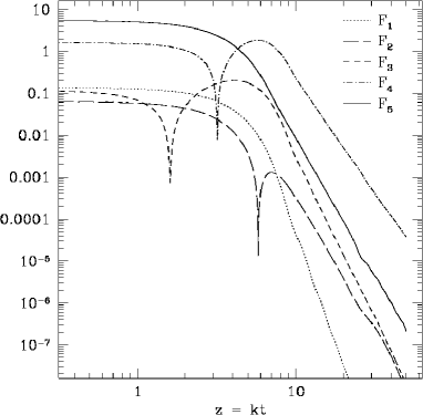
Figure 20: The functions $|F_{i}(z,1)|$ are shown left. The zeros are visible as spikes in the log-plot (Further below, at $z\sim 30$, also $F_{1}$ passes through zero.). Right, the functions $|A_{i}(r)|=|F_{i}(0,r)|$ are shown. As discussed in the text, all of them except $A_{3}$ are symmetrical under $r\rightarrow 1/r$.

All the functions, except $F_{5}$ which is constrained by Eq. (148) pass through $0$ (For $F_{1}$ the passage through $0$ is not visible on the plot since it occurs only at $z\simeq 30$). The asymptotic behavior of the functions can be obtained analytically. The same is true for the functions $A_{1}$ to $A_{5}$. As argued above, all the functions $A_{i}$ except $A_{3}$ are symmetric under $r\rightarrow 1/r$.

6.1.1 Scalar, vector and tensor decomposition and CMB anisotropies

The energy momentum tensor of seeds can be split into scalar, vector and tensor perturbations, since the time evolution of each of these components is independent. Furthermore, due to statistical isotropy, the scalar, vector and tensor modes are uncorrelated.

We use the decomposition of $\Theta_{ij}$ given in Chapter 3, Eqs. (41-46) The functions $F_{1}$ to $F_{5}$ determine the correlations: To work out the correlation functions we use also Eqs. (47,48) and (51,52) as well as (54). Using these identities and the ansatz (147), one easily verifies

$$\langle f_{p}(\tau)w_{i}^{*}(\tau^{\prime})\rangle = \langle f_{\pi}(\tau)w_{i}^{*}(\tau^{\prime})\rangle=\langle f_{p}(\tau)\tau_{ij}^{*}(\tau^{\prime})\rangle=0$$ (155)

$$\langle f_{\pi}(\tau)\tau_{ij}^{*}(\tau^{\prime})\rangle = \langle w_{i}(\tau)\tau_{jl}(\tau^{\prime})\rangle=0$$ (156)

$$\langle f_{p}(\tau)f_{p}^{*}(\tau^{\prime})\rangle = {1\over 3\sqrt{\tau\tau^{\prime}}}[2F_{5}(z^{2},r)+3F_{4}(z^{2},r)$$ (157)

$$+z^{2}(F_{3}(z^{2},r)/r+F_{3}(z^{2},1/r)r)+$$

$${4\over 3}z^{2}F_{2}(z^{2},r)+{1\over 3}z^{4}F_{1}(z^{2},r)]$$

$$\langle f_{\pi}(\tau)f_{\pi}^{*}(\tau^{\prime})\rangle = {1\over\sqrt{\tau\tau^{\prime}}k^{4}}[3F_{5}+4z^{2}F_{2}+z^{4}F_{1}]$$ (158)

$$\langle f_{p}(\tau)f_{\pi}^{*}(\tau^{\prime})\rangle=$$ (159)

$$-\sqrt{\tau\tau^{\prime}}[{1\over 3}z^{2}F_{1}(z^{2},r)+{4\over 3}F_{2}(z^{2},r)+rF_{3}(z^{2},1/r)]$$

$$\langle w_{i}(\tau)w_{j}^{*}(\tau^{\prime})\rangle=$$ (160)

$${4\over k^{4}\sqrt{\tau\tau^{\prime}}}[F_{5}+z^{2}F_{2}](k^{2}\delta_{ij}-k_{i}k_{j})$$

$$\langle\tau_{ij}(\tau)\tau^{*}_{lm}(\tau^{\prime})\rangle=$$ (161)

$${1\over\sqrt{\tau\tau^{\prime}}}F_{5}[\delta_{il}\delta_{jm}+\delta_{im}\delta_{jl}-\delta_{ij}\delta_{lm}+k^{-2}(\delta_{ij}k_{l}k_{m}+$$

$$\delta_{lm}k_{i}k_{j}-\delta_{il}k_{j}k_{m}-\delta_{im}k_{l}k_{j}-\delta_{jl}k_{i}k_{m}-\delta_{jm}k_{l}k_{i})+$$

$$k^{-4}k_{i}k_{j}k_{l}k_{m}]~{}.$$

It is interesting to note that although $\widehat{C}_{ijlm}$ is analytic, the correlation functions of the scalar, vector and tensor components, in general, are not. The reason for that is that the projection operators onto these components are not analytic [45]. This is important. It implies, e.g., that the anisotropic stresses in general have a white noise and not a $k^{4}$ spectrum as erroneously concluded in [105, 73]. The scalar anisotropic stress potential thus diverges on large scales, $\langle|f_{\pi}|^{2}\rangle\propto 1/(\tau k^{4})$ for $k\tau\ll 1$. A result which is also obtained in the large-$N$ limit and in numerical simulations of $O(N)$ models. The power spectrum of the scalar anisotropic stress potential $f_{\pi}$ is analytic if vector and tensor perturbations are absent, $F_{5}=F_{2}=0$. In the generic situation, $F_{5}(z=0,r=1)=A_{5}(1)\neq 0$.

Another situation where $f_{\pi}$ has a white noise spectrum is the case of perfectly coherent seeds [46], in other words if

$$\widehat{C}_{ijlm}(\mbox{\boldmath$k$},\tau,\tau^{\prime})=A_{ij}(\mbox{\boldmath$k$},\tau)A_{lm}^{*}(\mbox{\boldmath$k$},\tau^{\prime}).$$ (162)

The fact that as well $\langle f_{p}f_{p}^{*}\rangle$ as $\langle f_{p}f_{\pi}^{*}\rangle$ are white noise implies that also $\langle f_{\pi}f_{\pi}^{*}\rangle=\pm|\langle f_{p}f_{\pi}^{*}\rangle|^{2}/\langle f_{p}f_{p}^{*}\rangle$ must behave like white noise and thus $F_{5}\propto z^{4}$ and $F_{2}\propto z^{2}$ on large scales. This can also be obtained by using the analytic properties of the correlators $\langle\Theta_{0\mu}\Theta_{\alpha\beta}^{*}\rangle$ and energy momentum conservation [38].

Generically, we expect the following relation between scalar, vector and tensor perturbations of the gravitational field on super-horizon scales, $x\equiv k\tau\ll 1$: (The equations for the scalar, vector and tensor gravitational potentials in terms of $f.$, w and $\tau_{ij}$ are given in Chapter 3.)

$$\langle|\Phi-\Psi|^{2}\rangle \sim {12\epsilon^{2}\over\tau k^{4}}A_{5}(1)$$ (163)

$$\langle|\Sigma_{i}|^{2}\rangle \sim {16\epsilon^{2}\tau\over k^{2}}A_{5}(1)$$ (164)

$$\langle|H_{ij}|^{2}\rangle \sim 4\epsilon^{2}\tau^{3}A_{5}(1)~{}.$$ (165)

If the large scale CMB anisotropies were solely induced by super horizon perturbations, this could be translated into a ratio between the scalar, vector and tensor contributions to the $C_{\ell}$’s on large scales, $\ell\stackrel{{\scriptstyle<}}{{\sim}}50$. However, since the main contribution to the CMB anisotropies is induced at horizon crossing, $x=1$ (see below) the above relations cannot be translated directly and we can just learn that one expects, in general, contributions of the same order of magnitude from scalar, vector and tensor perturbations.

We want to discuss in some detail the CMB anisotropies induced from scalar perturbations. From

$$\Phi+\Psi=-2\epsilon f_{\pi}~{},$$ (166)

we see that even if $\Phi$ has a white noise spectrum due to ’compensation’ [49], this generically leads to a $k^{-4}$ spectrum for $\Psi$ and for the combination $\Phi-\Psi$ which enters in Eq. (167) below.

This finding is in contradiction with [105, 73], which predict a white noise spectrum for $\Psi$, but it is not in conflict with the Harrison Zel’dovich spectrum of CMB fluctuations which has been obtained numerically in [117, 51, 4]. This can be seen by the following simple argument: Since topological defects decay inside the horizon, the Bardeen potentials on sub-horizon scales are dominated by the contribution from dark matter and thus roughly constant. The integrated Sachs Wolfe term then contributes only up to horizon scales. Therefore, using the fact that for defect models $D_{g}$ and $V$ are smaller than the Bardeen potentials on super-horizon scales, we obtain

$$(\Delta T/T)_{\ell}(k)|_{SW}\sim(\Phi-\Psi)(k,x_{dec})j_{\ell}(x_{0}-x_{dec})$$ (167)

$$+\int_{x_{dec}}^{1}({\Phi}^{\prime}-{\Psi}^{\prime})(k,x)j_{\ell}(x_{0}-x)dx~{},$$

where $x=k\tau$ and prime stands for derivative w.r.t. $x$. The lower boundary of the integrated term roughly cancels the ordinary Sachs Wolfe contribution and the upper boundary leads, to

$$k^{3}\langle|(\Delta T/T)_{\ell}(k)|^{2}\rangle|_{SW}\sim$$

$$\quad\quad\epsilon^{2}[3F_{5}(1)+4F_{2}(1)+F_{3}(1)]j_{\ell}^{2}(x_{0}),$$ (168)

a Harrison-Zel’dovich spectrum. The main ingredients for this result are the decay of the sources inside the horizon as well as scaling, the rest follows for purely dimensional reasons.

The parameter space of generic causal scalar seed models provided by the five functions $F_{1}$ to $F_{5}$ (of two variables) is still enormous and is rather impossible to investigate. For a realistic model, the parameter space is even larger due to the radiation-matter transition which breaks scale invariance: the seed functions can be different in the radiation and in the matter era. For global $O(N)$ defects this difference turns out not to be very important (less than about 20% [47]) it may, however, go to factors of two and more for cosmic strings [132].

6.2 Mimicking inflation

Neil Turok has constructed a model with scaling causal seeds which perfectly reproduces the CMB anisotropy spectrum of inflationary models [144]. Other synthesized causal seed models with various heights of the acoustic peaks are discussed in [49, 46]. Spergel & Zaldarriaga argued that causal seeds can nevertheless be distinguished from inflationary models by the induced polarization [135]. In their argument they however use that the correlator $\langle f_{\pi}f_{\pi}\rangle$ be white noise. As we have seen, this is only correct for purely scalar or perfectly coherent seeds. Therefore, allowing for vector and tensor contributions, as well as for decoherence, one can in principle circumvent the Spergel & Zaldarriaga argument. However, the fact that seeds notoriously lead to too low amplitude acoustic peaks, limits very strongly the allowed vector and tensor contributions which enhance the CMB anisotropy spectrum in the Sachs-Wolfe, but not in the acoustic peak region. Furthermore, the smearing out of the acoustic peaks induced by decoherence is not observed in the data, limiting the allowed amount of decoherence considerably.

We restrict the following discussion to ’perfectly coherent’ models with purely scalar perturbations. We parameterize the seeds by

$$\langle\Psi_{s}(\mbox{\boldmath$k$},\tau)\Psi_{s}^{*}(\mbox{\boldmath$k$},\tau^{\prime})\rangle = {\epsilon^{2}\over\sqrt{\tau\tau^{\prime}}k^{4}}P_{1}(z,r)$$ (169)

$$\langle\Phi_{s}(\mbox{\boldmath$k$},\tau)\Phi_{s}^{*}(\mbox{\boldmath$k$},\tau^{\prime})\rangle = {\epsilon^{2}\over\sqrt{\tau\tau^{\prime}}k^{4}}P_{2}(z,r)$$ (170)

$$\langle\Psi_{s}(\mbox{\boldmath$k$},\tau)\Phi_{s}^{*}(\mbox{\boldmath$k$},\tau^{\prime})\rangle = {\epsilon^{2}\over\sqrt{\tau\tau^{\prime}}k^{4}}P_{3}(z,r)~{}.$$ (171)

Perfect coherence then implies

$$P_{3}(z,r)=\pm\sqrt{P_{1}(\sqrt{z^{2}r},1)P_{2}(\sqrt{z^{2}/r},1)}$$ (172)

Due to the absence of vector and tensor perturbations, the sum $\Phi+\Psi\propto f_{\pi}$ is suppressed by a factor $z^{2}$ on large scales, $z\ll 1$ [45]. In a first attempt we simply set $\Psi=-\Phi$, which implies $P_{1}=P_{2}=-P_{3}\equiv P$.

We discuss two families of models (see [48]).
Family I
To enhance the acoustic peak, we use seeds which are larger in the radiation era than in the matter era.

$$P_{r}(z,1) = {t\over 1+(bz)^{6}}$$ (173)

$$P_{m}(z,1) = {1\over 1+(bz)^{6}}~{},$$ (174)

where here the subscripts _r and _m indicate the radiation and matter era respectively. The parameters $t$ and $b$ are varied to obtain the best fit and the amplitude $\epsilon$ is determined by the overall normalization.
Family II
The second family of models is inspired by Ref. [144], which studies spherical exploding shells with $\rho+3p\propto\delta(r-A\tau)$. In terms of the source functions defined in Chapter 3, this model is characterized by

$$f_{\rho}\!+\!3f_{p} = {1\over\alpha\tau^{1/2}}{\sin(Ak\tau)\over Ak\tau}$$

$$f_{v} = {E(\tau)\over k^{2}\tau^{3/2}}{3\over C^{2}}\left[\cos(Ck\tau)-{\sin(Ck\tau)\over Ck\tau}\right]$$

with $\alpha=(\dot{a}/a)\tau$ and $E=(4-2/\alpha)/(3-12\alpha)$. The functions $f_{\rho}$ and $f_{\pi}$ are then determined by energy momentum conservation, Eqs. (49,50). The function $E$ is chosen such that the power spectrum of $f_{\pi}$ is white noise on super horizon scales, a condition which is required for purely scalar causal seeds as we have seen in the previous section. This leads to the Bardeen potentials

$$\Phi = {\epsilon\over k^{2}}(f_{\rho}+3{\alpha\over\tau}f_{v})~{},$$ (175)

$$\Psi = -\Phi-2\epsilon f_{\pi}~{}.$$ (176)

Here the seed functions are actually not given as random variables but as square-roots of power spectra, and one has always to keep in mind that we assume perfect coherence. Of course one can also regard Eqs. (175,176) as mere definitions with

$$P_{1}(z,1) = \tau k^{4}\Psi^{2}/\epsilon^{2}~{},$$ (177)

$$P_{2}(z,1) = \tau k^{4}\Phi^{2}/\epsilon^{2}~{},$$ (178)

$$P_{3}(z,1) = \tau k^{4}\Psi\Phi/\epsilon^{2}=-\sqrt{P_{1}(z,1)P_{2}(z,1)}~{}.$$ (179)

With a somewhat lengthy calculation one can verify that $E$ is chosen such that $f_{\pi}\propto$ const. for $z\ll 1$ and the functions $P_{i}(z,1)$ are analytic in $z^{2}=(k\tau)^{2}$. This family of models is described by the parameters $A$ and $C$, which have to satisfy $0<A,~{}C\leq 1$ for causality. Also here one can choose different amplitudes for the source functions in the radiation and matter era by introduction of the additional parameter $t\neq 1$.

Seeds generically produce isocurvature perturbations. For a flat universe, this implies a position of the first peak at $\ell\sim 350$, which is definitely incompatible with the recent CMB observations (see also [120], [53]). However, the tight constraints on the flatness of the universe obtained from CMB data analysis are based on the assumption of adiabatic primordial fluctuations. Using this loophole, it is possible to construct closed $\Lambda$-dominated isocurvature models which have the first acoustic peak in the observed position.

For a given seed-model, the position of the first acoustic peak is determined primarily by the angle subtended by the acoustic horizon $\lambda_{ac}$ at decoupling time, $\tau_{dec}$. The angle under which a given comoving scale $\lambda$ at conformal time $\tau_{dec}$ is seen on the sky is given by $\theta(\lambda)=\lambda/\chi(\tau_{0}-\tau_{dec})$, where

$$\chi(y)=\left\{\begin{array}[]{ll}\sin(y)&\mbox{ if }~{}~{}K>0\\ \sinh(y)&\mbox{ if }~{}~{}K<0\\ y&\mbox{ if }~{}~{}K=0~{}.\end{array}\right.$$

is the comoving angular diameter distance (K denotes the curvature of 3-space). As the harmonic number $\ell$ is inversely proportional to the angle $\theta$, this yields $\ell_{\rm peak}\simeq R\ell_{\rm peak}^{\rm flat}$  where  $R=\theta_{ac}^{\rm flat}/\theta_{ac}$ and $\ell_{\rm peak}^{\rm flat}$ is the peak position in a flat model with the same value of $\Omega_{m}h^{2}$. In terms of cosmological parameters one finds (see Ref. [16] or [48], a factor $1/2$ is missing in the formula of [16]),

$$R=\frac{1}{2}\sqrt{\frac{\Omega_{m}}{|\Omega_{K}|}}\chi(\tau_{0}-\!\tau_{\rm dec}).$$

An interesting point is that for $\Omega_{m}\rightarrow 0$ the quantity $R$ depends very sensitively on $\Omega_{\Lambda}$. Thus, we can have important shifts in the power spectrum, $R\sim 0.6$ say, with relatively small deviations from flatness ($\Omega_{m}=0.3$, $\Omega_{\Lambda}=0.9$, $\Omega_{K}=-0.2$). In Ref. [16] the authors have shown that the simple prescription $\ell\rightarrow R\ell$ reproduces the CMB power spectra for curved universes within a few percent. On lines of constant $R$, CMB power spectra are nearly degenerate. This simple prescription can be used to rescale the flat spectrum. Furthermore, one has to ascertain that the value of $h^{2}\Omega_{m}$ used in the spectrum calculation agrees roughly with the value preferred by the best fit value of $R$ and the super-novae constraint [125], which can be cast in the form $\Omega_{m}\simeq 0.75\Omega_{\Lambda}-0.25$. $h^{2}\Omega_{m}$ determines the time of equal matter and radiation and thus influences the early integrated Sachs-Wolfe effect, which contributes to the spectrum right in the region of the first peak. We therefore get a better approximation if we use the correct value for $\Omega_{m}h^{2}$.

The results from an analysis of family I are shown in Figs. 21 and 22 (long dashed lines). The best fit model is shown. Clearly, even though we can change the cosmological parameters to fit the first acoustic peak, the second and third peaks are also shifted by this procedure and can no longer be fitted. The cosmological parameter $R$ is now fixed by CMB anisotropy measurements due to the measured inter-peak distance. This situation was still slightly different with the ’old’ Boomerang and Maxima data [35, 68] for which this model could still provide a reasonable fit [48]. in addition, the shifted first peak is too narrow to fit the data well.

The ’best fit’ model corresponds to the parameters $t=2.2,~{}b=1/9,~{}\Omega_{m}=0.35$ and $R=0.53$. It has a value of $\chi^{2}=96$, which, for $13$ points and $4$ parameters ($t$, $b$, $R$ and the normalization), excludes it at more than $99.8\%$ c.l. if Gaussian statistics are assumed.

Figure 21: The CMB temperature anisotropy spectrum $\ell(\ell+1)C_{\ell}^{(T)}$ for our best fit model of family I (long dashed) and family II (solid) is compared with the new B98 data. Family I model is closed, $\Omega\sim 1.2$ it has problems fitting anything. The family II model is flat and is in good agreement with the data ($\chi^{2}=4/9$), we fitted only $\ell\leq 700$. A standard inflationary spectrum with the same cosmological parameters as the family II model ($h=0.65,~{}h^{2}\Omega_{b}=0.019,~{}\Omega_{cdm}=0.35,~{}\Omega_{\Lambda}=1-\Omega_{m}$) is also indicated (dotted).

Figure 22: The CMB polarization spectrum $C_{\ell}^{(E)}$s for our best fit model of family I (long dashed) and family II (solid) is compared with a standard inflationary spectrum with the same parameters as above (dotted). The family I model predicts a larger polarization signal in the band $50\leq\ell\leq 500$. On the contrary, the lack of intermediate scale polarization at $\ell\leq 200$ in the family II model is clearly visible.

A much better fit can be achieved by the models of family II. The best fit model of this family has $\chi^{2}=4.0$ for $13$ points and $5$ parameters ($A,~{}C,~{}t,~{}R$ and the normalization) and is in good agreement with the data (see Fig. 21, solid line). The model shown corresponds to the best fit parameters $A=0.9,~{}C=0.8,~{}t=0.9,$ and $R=1$. In this model which is flat and causal, the first peak in the polarization spectrum is suppressed, as has been noted in Ref. [135] (see Fig. 22, solid line).

We can therefore conclude that generic causal scaling seed models for structure formation can reproduce the recent CMB anisotropy data [35, 68]. To achieve this agreement, we have suppressed vector and tensor perturbations and have assumed perfectly coherent fluctuations. We believe that it is quite improbable that topological defects from a GUT phase transition have such a behavior. Nevertheless, there might be some other scale-invariant causal physical mechanism (e.g. some spherically symmetric ’neutrino explosions’, see Ref. [144]) leading to seeds of this or similar type. Clearly, we only have a satisfactory model of structure formation if also the physical origin of the ’seeds’ is clarified.

6.3 Mixed models

In this section we want to discuss the possibility of combining topological defects with primordial, inflationary perturbations. There are at least two important reasons why such an analysis is interesting. First of all, as we saw in the previous chapters, the predictions based on topological defect models for the CMB power spectra are dramatically different from what is expected in the standard inflationary model. This means that, in principle, the two contributions can be disentangled. Secondly, this analysis contributes in a phenomenological but physically motivated way to the discussion, about the model dependence of the values of cosmological parameters derived from accurate CMB data. Inflationary models leading to a mixture of inflationary perturbations and defects which both contribute to the CMB anisotropies have been developed e.g.  in Refs. [79, 32, 87] and others. A similar analysis, but with cosmic string and with an older CMB dataset, can be found in [27]. A mixture of global defects and inflationary perturbations has also been considered in [19].

We consider an initial fluctuation spectrum with scalar initial perturbations given by their spectral index $n_{s}$, in addition to topological defects which formed at some symmetry breaking temperature $T_{c}$ determining the amplitude of the seed perturbations. For definiteness we take the defects to be cosmic texture. It is reasonable to assume that the inflationary fluctuations and those induced by topological defects are not correlated and therefore the resulting perturbation spectra can be added in quadrature. We set

$$C_{\ell}=\left[{1\over(1+r)}C_{\ell}^{I}+{{r}\over(1+r)}C_{\ell}^{D}\right]AC_{10}^{COBE}$$ (180)

for the CMB anisotropy, where $A$ is the pre factor in units of $C_{10}^{COBE}$, $C_{10}^{I}=C_{10}^{D}=1$ and the parameter $r$ gives the relative amplitude of textures/inflation at $\ell=10$. We let vary the cosmological parameters as follows: $\Omega_{m}=0.015$ to $1.0$; $\Omega_{b}=0.015$ to $0.2$; $\Omega_{\Lambda}=0.0$ to $1.0$ and $h=0.25$ to $0.95$. We restrict the analysis to flat universes. We vary the spectral index of the primordial inflationary perturbations within the range $n_{s}=0.50$ to $1.50$. The theoretical inflationary models are computed using the publicly available cmbfast program and are compared with the recent BOOMERanG-98 [110], DASI [66] and MAXIMA-1 [97] results. The power spectra from these experiments were estimated in $19$, $12$ and $10$ bins respectively, spanning the range $25\leq\ell\leq 1000$. For the DASI and MAXIMA-I experiments, we use the public available correlation matrices and window functions. For the BOOMERanG experiment, we assign a flat window function in each bin $\ell(\ell+1)C_{\ell}/2\pi=C_{B}$, we approximate the signal $C_{B}$ to be a Gaussian variable, and we consider $\sim 10\%$ correlations between neighboring bins. The likelihood for a given cosmological model is then defined by $-2{\rm ln}L=(C_{B}^{th}-C_{B}^{ex})M_{BB^{\prime}}(C_{B^{\prime}}^{th}-C_{B^{\prime}}^{ex})$ where $M_{BB^{\prime}}$ is the Gaussian curvature of the likelihood matrix at the peak. We consider $10\%$, $4\%$ and $5\%$ Gaussian distributed calibration errors for the BOOMERanG-98, DASI and MAXIMA-1 experiments respectively. We also include the COBE data using Lloyd Knox’s RADPack packages [166].

In Fig. 23 we plot the obtained likelihood distribution for the parameter $R$, after marginalization over the remaining ’nuisance’ parameters and as function of different external priors. The present CMB data plus an external Gaussian prior on the value of the Hubble constant $h=0.65\pm 0.2$ gives $r<2.6$ at $95\%$ c.l.. Hence, we cannot exclude a substantial admixture of topological defects from CMB data alone. Adding strong constraints on the baryon density parameter from big bang nucleosynthesis $\Omega_{b}h^{2}=0.020\pm 0.004$ gives $r<2.1$. Finally, combining the CMB data with LSS observation by including a constraint $\sigma_{8}\Omega_{m}^{0.5}=0.50\pm 0.05$ gives $r<1.6$, always at $95\%$ c.l.. As we can see, even assuming quite restrictive priors, the present CMB data allow a contribution from textures as big as $r\sim 1$. Furthermore, models with non-zero $r$ are in slightly better agreement with the data, but there is no significant evidence for non-vanishing $r$.

The main result of this analysis is that current microwave background data do not exclude a dominant contribution from textures on large scales, and marginally favor a significant fraction.

It is interesting to study how textures can affect the constraints on the remaining cosmological parameters. Marginalizing over $\Omega_{m},~{}\Omega_{\Lambda},~{}h$ and $\Omega_{b}$. Assuming the external priors $h=0.65\pm 0.2$ and $\Omega_{b}h^{2}=0.020\pm 0.002$, we obtain the likelihood contours shown in Fig. 24 (left panel) in the $r$– $n_{s}$ parameter space. There is a degeneracy between the amplitude of the texture component and the spectral tilt. A blue tilt ($n_{s}>1$) is found to be compatible with a larger textures contribution.

If we instead marginalize over $\Omega_{m},~{}\Omega_{\Lambda},n_{S}$, without assuming external priors from big bang nucleosynthesis, we find the contours shown in Fig. 24 (right panel) in the $r$ – $\Omega_{b}h^{2}$ plane. Without the BBN constraint, the contribution of textures modes can be even larger, and there is clearly a degeneracy along the $r-\Omega_{b}h^{2}$ direction.

The best fit spectrum with $\Omega_{m}=0.175,~{}\Omega_{\Lambda}=0.825,~{}h=0.75,~{}\Omega_{b}=0.045,n_{s}=1.02,~{}r=0.9$ together with a ’concordance’ fit, $\Omega_{m}=0.3,~{}\Omega_{\Lambda}=0.7,~{}h=0.65,~{}\Omega_{b}=0.04,n_{s}=1,~{}r=0$ are shown in Fig. 25.

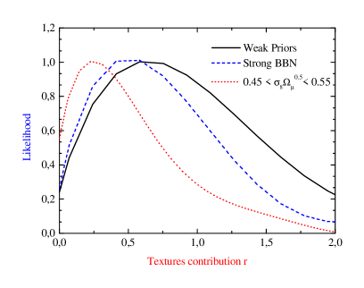
Figure 23: The likelihood probability distribution functions for $r$ in the case of different external priors.

  

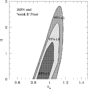
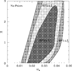
Figure 24: Left: the likelihood contours for $r$ and $n_{s}$ are shown after marginalization over $\Omega_{m},~{}h,~{}\Omega_{b}$ and $\Omega_{\Lambda}$ with weak priors on $h$ and $\Omega_{b}$ (see text). Right: the likelihood contours for $r$ and $\omega_{b}=\Omega_{b}h^{2}$ are shown after marginalization over $n_{s},~{}\Omega_{m},~{}h$ and $\Omega_{\Lambda}$. No priors are applied

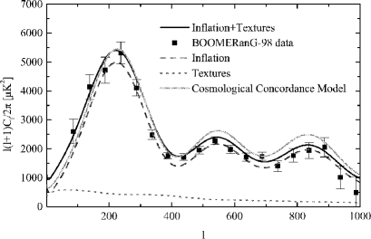
Figure 25: The best fit mixed spectrum is shown. The corresponding parameters are $\Omega_{m}=0.175,~{}\Omega_{\Lambda}=0.825,~{}h=0.75,~{}\Omega_{b}=0.045,n_{s}=1.02,~{}r=0.9$. Its inflationary (long dashes) and texture (short dashes) components as well as the spectrum from a concordance model (dotted, see text) are also indicated.

7 Conclusion

In this review we have discussed the role of topological defects for cosmic structure formation. Even though the basic idea seems natural and intriguing, we have seen that structure formation with global $O(n)$ defects and (local) cosmic strings is ruled out already by the CMB anisotropy data alone. Due to the isocurvature nature of the perturbations and due to the importance of vector and tensor perturbations, defects do not induce the acoustic peaks visible in present data. Furthermore, non-linearities in the defect evolution tend to decohere, smear out, the peak structure. Nevertheless, generic causal seeds, which are dominated by scalar perturbations and have nearly no decoherence, may mimic the CMB anisotropy spectrum of inflationary models. Such models, however, do certainly not represent topological defects for which non-linearity and therefore decoherence is one of the basic ingredients. Furthermore, such models could be distinguished by their polarization spectrum. Models where both, inflation and topological defects play a role for structure formation, such that the large scale CMB anisotropies from both components are of comparable amplitude, cannot be excluded with present data.
Acknowledgment
We thank all our colleagues for the many discussions on the subject which contributed to this report. Especially we want to mention: Robert Brandenberger, Nathalie Deruelle, Paolo deBernardis, Pedro Ferreira, Mark Hindmarsh, Tom Kibble, Joao Magueijo, Ue-Li Pen, Patrick Peter, Mairi Sakellariadou, Uros Seljak, David Spergel, Danièle Steer, Neil Turok, Jean-Philippe Uzan, Tanmay Vachaspati, Alex Vilenkin and Nicola Vittorio.
This work has been supported by the European network CMBNET and by the Swiss NSF. RD thanks the Institute for Advanced Study for hospitality and the Monell Foundation for financial support. APPENDIX

Appendix A Definitions of all gauge-invariant perturbation variables

In this Appendix we give precise definitions of all the gauge-invariant perturbation variables used in the text. These definitions, their geometrical interpretation and a short derivation of the perturbation equations can be found in Refs. [42, 91]. We restrict the analysis to the spatially flat case, $K=0$. The general case can be found in the references above. We define the perturbed metric by

$$g=\bar{g}+a^{2}h~{},$$ (181)

where $\bar{g}$ denotes the standard Friedman background, $a$ is the scale factor and $h$ denotes the metric perturbation.

A.1 Scalar perturbations

Scalar perturbations of the metric are of the form

$$h^{(S)} = -2A(d\tau)^{2}+2iBk_{j}d\tau dx^{j}+2(H_{L}+{1\over 3}H_{T})\delta_{ij}dx^{i}dx^{j}$$ (182)

$$-2k^{-2}H_{T}k_{i}k_{j}dx^{i}dx^{j}~{}.$$

Computing the perturbation of the Ricci curvature scalar and the shear of the equal time slices, we obtain

$$\delta\mbox{\boldmath$R$}=4a^{-2}k^{2}{\cal R} {\cal R}=H_{L}+{1\over 3}H_{T}$$ with (183)

$$\Sigma=a\sigma({k_{i}k^{j}\over k^{2}}-{1\over 3}\delta_{i}^{j})dx^{i}\otimes\partial_{j}, \sigma={1\over k}\dot{H}_{T}-B~{}.$$ with (184)

The Bardeen potentials are the combinations

$$\Phi = {\cal R}-(\dot{a}/a)k^{-1}\sigma$$ (185)

$$\Psi = A-k^{-1}[(\dot{a}/a)\sigma-\dot{\sigma}]\;.$$ (186)

They are invariant under infinitesimal coordinate transformations (gauge transformations). In longitudinal gauge defined by $B=H_{T}=0$, the variable $\Phi$ represents the perturbation of the spatial metric while $\Psi$ is the perturbation of the $dt^{2}$ term, the lapse function.

To define perturbations of the most general energy momentum tensor, we introduce the energy density $\rho$ and the energy flux $u$ as the time-like eigenvalue and normalized eigenvector of $T^{\mu}_{\nu}$,

$$T_{\mu}^{\;\;\nu}u^{\mu}=-\rho u^{\nu}\;\;,\;\;u^{2}=-1\;.$$

We then define the perturbations in the energy density and energy flux field by

$$\rho=\overline{\rho}(1+\delta)\;\;,$$ (187)

$$u=u^{0}\partial_{t}+u^{i}\partial_{i}~{};$$ (188)

$u^{0}$ is fixed by the normalization condition, $u^{0}=a^{-1}(1-A)$ and $\overline{\rho}$ is the homogeneous background energy density.. In the 3–space orthogonal to $u$ we define the stress tensor by

$$\tau^{\mu\nu}\equiv P^{\mu}_{~{}~{}\alpha}P^{\nu}_{~{}~{}\beta}T^{\alpha\beta}~{},$$ (189)

where $P=u\otimes u+g$ is the projection onto the sub–space of $T{\cal M}$ normal to $u$. It is

$$\tau^{0}_{0}=\tau^{0}_{i}=\tau^{i}_{0}=0~{}.$$

The perturbations of pressure and anisotropic stresses can be parameterized by

$$\tau_{i}^{\;j}=\bar{p}[(1+\pi_{L})\delta_{i}^{\;j}+\pi_{i}^{\;\;j}]~{}~{}\mbox{ , with }~{}\pi^{i}_{i}=0\;,$$ (190)

where $\bar{p}$ is the background pressure. For scalar perturbations we set

$$u^{0} = (1-A)\;,\;{u^{(S)j}\over u^{0}}=-i{k^{j}\over k}v$$

and

$$\pi^{(S)i}_{~{}j} = (-k^{-2}k^{i}k_{j}+{1\over 3}\delta^{i}_{~{}j})\Pi~{}.$$

Studying the behavior of these variables under gauge transformations, one finds that the anisotropic stress potential $\Pi$ is gauge invariant. Another gauge invariant combination from the matter variables alone is

$$\Gamma=\pi_{L}-{c_{s}^{2}\over w}\delta~{}.$$ (191)

$\Gamma$ is proportional to the divergence of the entropy flux and vanishes for adiabatic perturbations [50]. A gauge invariant velocity variable is the shear of the velocity field,

$$\sigma^{(Sm)}_{ij}=(k^{-2}k_{i}k_{j}-{1\over 3}\delta_{ij})a^{3}V\mbox{ , ~{}with }~{}~{}V=v-k^{-1}\dot{H}_{T}.$$ (192)

There are several different useful choices of gauge invariant density perturbation variables,

$$D_{s} = \delta+3(1+w)(\dot{a}/a)k^{-1}\sigma$$ (193)

$$D_{g} = \delta+3(1+w){\cal R}=D_{s}+3(1+w)\Phi$$ (194)

$$D = D_{s}+3(1+w)(\dot{a}/a)k^{-1}V\;.$$ (195)

In this work we mainly use $D_{g}$. Here $w=p/\rho$ denotes the enthalpy. Clearly, these matter variables can be defined for each matter component separately. For ideal fluids like CDM or the baryon-photon fluid long before decoupling, anisotropic stresses vanish and $\pi_{L}=(c_{s}^{2}/w)\delta$, where $c_{s}$ is the adiabatic sound speed.

Also scalar perturbations of the photon brightness, $\iota^{(S)}$ are not gauge invariant. To define the brightness we first consider the one particle photon distribution function

$$f(x,\mbox{\boldmath$p$})=\bar{f}(\tau,p)+F(\tau,\mbox{\boldmath$x$},\mbox{\boldmath$p$})~{},$$

where $\bar{f}$ is just the Bose-Einstein distribution. The background Liouville equation requires that $\bar{f}$ be a function of the redshift corrected momentum $v=ap$ only. The brightness perturbation is then the momentum integral of $F$, which depends on the photon direction, position and time

$$\iota(\mbox{\boldmath$n$},\mbox{\boldmath$x$},\tau)={4\pi\over\bar{\rho}}\int dpp^{3}F(\mbox{\boldmath$p$},\mbox{\boldmath$x$},\tau)~{}.$$ (196)

This can be decomposed in scalar vector and tensor contributions,

$$\iota=\iota^{(S)}+\iota^{(V)}+\iota^{(T)}~{}.$$

It has been shown [42] that the combination

$${\cal M}^{(S)}=\iota^{(S)}+4{\cal R}+4ik^{-1}n^{j}k_{j}\sigma$$ (197)

is gauge invariant. This is the variable which we use here. In other work[74] the gauge invariant variable $\Theta\equiv{\cal M}+\Phi$ has been used. Since $\Phi$ is independent of the photon direction $n$ this difference in the definition shows up only in the monopole, $C_{0}$. But clearly, as can be seen from Eq. (197), also the dipole of $\iota^{(S)}$, $C_{1}$, is gauge dependent.

The brightness perturbation of the neutrinos is defined the same way and is not repeated here.

A.2 Vector perturbations

Vector perturbations of the metric are of the form

$$h^{(V)}=2B_{j}dx^{j}dt+ik^{-1}(k_{l}H_{j}+k_{j}H_{l})dx^{l}dx^{j}~{},$$ (198)

where $B$ and $H$ are transverse vector fields. The simplest gauge invariant variable describing the two vectorial degrees of freedom of metric perturbations is $\Sigma$,

$$\Sigma_{j}=k^{-1}\dot{H}_{j}-B_{j}~{}.$$ (199)

Vector anisotropic stresses are gauge invariant. They are of the form

$$\pi_{lj}^{(V)}=ik^{-1}(k_{j}\Pi_{l}+k_{l}\Pi_{j})~{}.$$ (200)

The vector degrees of freedom of the velocity field are cast in the vorticity

$$u_{l;j}-u_{j;l}=ia(k_{j}\omega_{l}-k_{l}\omega_{j})~{}\mbox{ with }~{}\omega_{j}=v_{j}-B_{j}~{}.$$ (201)

Vector perturbations of the photon brightness are gauge-invariant. To maintain the notation consistent we denote them by ${\cal M}^{(V)}\equiv\iota^{(V)}$.

A.3 Tensor perturbations

We define tensor perturbations of the metric by

$$h^{(T)}=2H_{ij}dx^{i}dx^{j}~{},$$ (202)

where $H_{ij}$ is a transverse traceless tensor field.

The only tensor perturbations of the energy momentum tensor are anisotropic stresses,

$$\pi_{ij}^{(T)}=\Pi_{ij}~{}.$$ (203)

Again for notational consistency tensor perturbations of the photon brightness are denoted ${\cal M}^{(T)}\equiv\iota^{(T)}$.

Clearly, all tensor perturbations are gauge-invariant (there are no tensor type gauge transformations).

Appendix B Boltzmann equation and polarization

The relativistic Boltzmann equation for the photon distribution function is of the form

$$p^{\mu}\partial_{\mu}f-\Gamma^{i}_{\alpha\beta}p^{\alpha}p^{\beta}\frac{\partial f}{\partial p^{i}}=C[f],$$ (204)

where $f(t,\mbox{\boldmath$x$},\mbox{\boldmath$p$})$ is the one-particle distribution function on the mass bundle $P_{m}=\{(p,x)\in T{\cal M}|g(x)(p,p)=-m^{2}\}$ and $C[f]$ is the collision integral which describes interactions. The left hand side of (204) requires the particles to move along geodesics in the absence of collisions. (For a thorough treatment of the kinetic approach in general relativity see e.g.  [139] or [147] and references therein.)

B.1 The collisionless case, momentum integrals

Let us first consider the situation where collisions are negligible, $C[f]=0$. The unperturbed Boltzmann equation then implies that $f$ be a function of $v=ap$ only. Setting $f=\bar{f}(v)+F(\tau,\mbox{\boldmath$x$},v,\mbox{\boldmath$n$})$, where $n$ denotes the momentum directions, leads to the perturbation equation

$$\partial_{\tau}F-n^{i}\partial_{i}F=v\frac{d\bar{f}}{dv}\left[n^{i}A_{,i}-n^{i}n^{j}\left(B_{i,j}-\dot{H}_{ij}\right)+H_{L}\right].$$ (205)

To derive (205) we have used $p^{2}=0$. The Liouville equation for particles with non-vanishing mass can be found in Ref. [42].

The ansatz

$$f(x,\mbox{\boldmath$p$})=\bar{f}\left(\frac{g^{(3)}(\mbox{\boldmath$p$},\mbox{\boldmath$p$})^{\frac{1}{2}}}{T(x,\mbox{\boldmath$n$})}\right)=\bar{f}\left(\frac{v}{T(x,\mbox{\boldmath$n$})}\right)$$ (206)

with $T(x,\mbox{\boldmath$n$})=\overline{T}(\tau)+\Delta T(x,\mbox{\boldmath$n$})$, and where $g^{(3)}$ is the spatial part of the metric, leads to

$$f=\bar{f}-v\frac{d\bar{f}}{dv}\frac{\Delta T}{\overline{T}}.$$ (207)

Note that in terms of the brightness perturbation, $\imath$ defined in AppendixA,

$$\imath=\frac{4\pi}{\bar{\rho}a^{4}}\int_{0}^{\infty}Fv^{3}dv~{}~{}~{}~{}\mbox{ we have }~{}~{}\frac{\Delta T}{T}=\frac{1}{4}\imath~{}.$$ (208)

Comparing this with equation (205), we obtain

$$\partial_{\tau}\left(\frac{\Delta T}{T}\right)+n^{i}\partial_{i}\left(\frac{\Delta T}{T}\right)=$$ (209)

$$-\left[n^{i}A_{|i}-\left(B_{i|j}-\dot{H}_{ij}\right)n^{i}n^{j}+H_{L}\right].$$

The fact that gravitational perturbations of Liouville’s equation can be cast entirely into temperature perturbations of the original distribution is not astonishing. This is just an expression of gravity being “achromatic”, i.e.  independent of the photon energy.

We now decompose (209) into scalar, vector and tensor components. Since components with spin higher than 2 are not sourced by the right hand side of equation (209) and since they are suppressed at early times, when collisions are important, we neglect them.

For the scalar contribution to $\Delta T/T$ we obtain from (209) (in Fourier space)

$$\partial_{\tau}\left(\frac{\Delta T}{T}\right)^{(S)}+in^{\ell}k_{\ell}\left(\frac{\Delta T}{T}\right)^{(S)}=$$ (210)

$$-\left[n^{i}A_{i}+n^{i}n^{j}k_{i}k_{j}\left(B-\dot{H}\right)+H_{L}+\frac{1}{3}k^{2}\dot{H}\right].$$

This equation is not manifestly gauge-invariant. However, defining

$$\frac{1}{4}{\cal M}^{(S)}=\left(\frac{\Delta T}{T}\right)^{(S)}+H_{L}+\frac{1}{3}k^{2}H+in^{\ell}k_{\ell}\left(\dot{H}-B\right),$$ (211)

it reduces to

$$\partial_{\tau}{\cal M}^{(S)}+\mu k{\cal M}^{(S)}=4i\mu k(\Phi\!-\!\Psi),$$ (212)

where $\Phi$ and $\Psi$ are the Bardeen potentials and we have set $\mu=n^{j}k_{j}/k$. Since the right hand side of (212) is gauge invariant, the left hand side must be so as well and we conclude that ${\cal M}^{(S)}$ is a gauge-invariant variable (a direct proof of this, analyzing the gauge transformation properties of the distribution function, can be found in [42]).

${1\over 4}{\cal M}^{(S)}$ coincides with the scalar temperature fluctuations up a to a gauge dependent monopole and dipole contribution.

The vector and tensor contributions to $\Delta T/T$ are gauge invariant by themselves and we denote them by ${1\over 4}{\cal M}^{(V)}$ and ${1\over 4}{\cal M}^{(T)}$. In the absence of collisions, they satisfy the equations

$$\dot{{\cal M}}^{(V)}+i\mu k{\cal M}^{(V)} = -4i\mu n^{m}k\Sigma_{m}^{(V)}$$ (213)

$$\dot{{\cal M}}^{(T)}+i\mu k{\cal M}^{(T)} = 4n^{\ell}n^{m}\dot{H}_{m\ell}.$$ (214)

The components of the energy momentum tensor are obtained by integrating the second moments of the distribution function over the mass shell,

$$T^{\mu\nu}=\int_{P_{m}(x)}p^{\mu}p^{\nu}f(p,x)\mu(x,p)~{},$$ (215)

with the invariant measure $\mu(x,p)={\sqrt{|\det(g)}|\over p^{0}}d^{3}p$. One finds

$$D_{g}^{(\gamma)} = \frac{1}{4\pi}\int{\cal M}^{(S)}d\Omega=\sigma_{0}^{(S)}={\cal M}_{0}^{(0)}~{},$$ (216)

$$V^{(\gamma)} = \frac{3i}{16\pi}\int\mu{\cal M}^{(S)}d\Omega=\frac{3}{4}\sigma_{1}^{(S)}=\frac{1}{4}{\cal M}_{1}^{(0)}~{},$$ (217)

$$\Pi^{(\gamma)} = \frac{-9}{8\pi}\int\left(\mu^{2}-\frac{1}{3}\right){\cal M}^{(S)}d\Omega=3\sigma_{2}^{(S)}=\frac{3}{5}{\cal M}_{2}^{(0)}~{},$$ (218)

$$\Gamma^{(\gamma)} = 0~{},$$ (219)

$$\mbox{\boldmath$V$}^{(V)} = \frac{1}{4\pi}\int\mbox{\boldmath$n$}{\cal M}^{(V)}d\Omega$$

$$= \frac{1}{3}\left(\sigma_{1,0}^{(V)}+\sigma_{1,2}^{(V)},\sigma_{2,0}^{(V)}+\sigma_{2,2}^{(V)},0\right)$$

$$= \frac{-1}{3\sqrt{2}}\left({\cal M}_{1}^{(+1)}+{\cal M}_{1}^{(-1)},i({\cal M}_{1}^{(+1)}-{\cal M}_{1}^{(-1)}),0\right)~{},$$

$$\mbox{\boldmath$\Pi$}^{(V)} = \frac{3}{2\pi}\int\mu\mbox{\boldmath$n$}{\cal M}^{(V)}d\Omega$$

$$= \frac{-6i}{5}\left(\sigma_{1,1}^{(V)}+\sigma_{1,3}^{(V)},\sigma_{2,1}^{(V)}+\sigma_{2,3}^{(V)},0\right)$$

$$= \frac{\sqrt{6}}{5}\left(i({\cal M}_{2}^{(+1)}+{\cal M}_{2}^{(-1)}),{\cal M}_{2}^{(+1)}-{\cal M}_{2}^{(-1)},0\right)~{},$$

$$\left(\Pi_{ij}^{(T)}\right) = \frac{3}{4\pi}\left(\int n_{i}n_{j}{\cal M}^{(T)}d\Omega\right)=\left(\begin{array}[]{ccc}-\pi^{(T)}_{+}&\pi^{(T)}_{\times}&0\\ \pi^{(T)}_{\times}&\pi^{(T)}_{+}&0\\ 0&0&0\end{array}\right)~{},$$ (225)

$$\mbox{with }~{}~{}~{}\pi_{i}^{(T)} = \frac{2}{35}\left(7\sigma_{0,i}^{(T)}+10\sigma_{2,i}^{(T)}+3\sigma_{4,i}^{(T)}\right)$$

$$\mbox{and }~{}~{}~{}\pi_{+}^{(T)} = \frac{-\sqrt{3}}{5\sqrt{2}}\left({\cal M}_{2}^{(+2)}+{\cal M}_{2}^{(-2)}\right)~{},$$

$$\pi_{\times}^{(T)} = \frac{-\sqrt{3}i}{5\sqrt{2}}\left({\cal M}_{2}^{(+2)}-{\cal M}_{2}^{(-2)}\right)$$

Here, we have also expressed the result in terms of the multipole moments defined by the expansions (273) and (266) for a wave vector $k$ pointing in $z$-direction..

The expressions for the neutrino fluid perturbations in terms of ${\cal N}$ are identical.

B.2 Collisions, polarization

Let us now turn to the collision term. Just before the process of recombination during which the fluid description of radiation breaks down, the temperature is $\sim 0.4\mathrm{~{}eV}$. The electrons and nuclei are non-relativistic and the dominant collision process is non-relativistic Thomson scattering.

Thomson scattering depends also on the polarization of the incoming radiation field. It is therefore necessary to treat polarization. This is usually done by introducing the Stokes parameters [78, 93, 107, 22]:

For a harmonic electro-magnetic wave with associated electric field

$${\bf E}(\mbox{\boldmath$x$},t)=\left({\mbox{\boldmath$\epsilon$}}_{1}E_{1}+{\mbox{\boldmath$\epsilon$}}_{2}E_{2}\right)e^{ip\mbox{\boldmath$n\cdot x$}-i\omega t}~{},$$ (226)

where $n$, $\mbox{\boldmath$\epsilon$}_{1}$ and $\mbox{\boldmath$\epsilon$}_{2}$ form an orthonormal basis and the complex field amplitudes are parameterized as $E_{j}=a_{j}e^{i\delta_{j}}$, the Stokes parameters are given by

$$I = a_{1}^{2}+a_{2}^{2}$$ (227)

$$Q = a_{1}^{2}-a_{2}^{2}$$ (228)

$$U = 2a_{1}a_{2}\cos(\delta_{2}-\delta_{1})$$ (229)

$$V = 2a_{1}a_{2}\sin(\delta_{2}-\delta_{1}).$$ (230)

$I$ is the intensity of the wave (whose perturbation ${\cal M}$ has interested us so far), while $Q$ is a measure of the strength of linear polarization (the ratio of the principal axis of the polarization ellipse). $U$ and $V$ give phase information (the orientation of the ellipse). $V$ also gives the amplitude of circular polarization. For non-relativistic Thomson scattering $V$ is completely decoupled and (since it vanishes at early times) is therefore never generated.

As $Q$ and $U$ vanish in the background, perturbations cannot couple to them (since such terms are 2nd order), and the equation corresponding to (210) for $Q$ and $U$ become (neglecting scattering)

$$\partial_{\tau}(Q;U)+in^{\ell}k_{\ell}(Q;U)=0.$$ (231)

The differential cross section of Thomson scattering for a photon with incident polarization ${\mbox{\boldmath$\epsilon$}}_{(i)}$ scattering into the outgoing polarization ${\mbox{\boldmath$\epsilon$}}_{(s)}\equiv{\mbox{\boldmath$\epsilon$}}^{\prime}$ is [78]

$$\frac{d\sigma}{d\Omega}=\frac{3}{8\pi}\sigma_{T}\left|{\mbox{\boldmath$\epsilon$}}_{(s)}^{*}{\mbox{\boldmath$\epsilon$}}_{(i)}\right|^{2}.$$ (232)

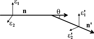
Figure 26: Definition of the angles and vectors for Thomson scattering in the $(\mbox{\boldmath$n$},{\mbox{\boldmath$\epsilon$}}_{2})$ plane.

It is often convenient to introduce the two ‘partial’ intensities $I_{1}\equiv a_{1}^{2}=(I+Q)/2$ and $I_{2}\equiv a_{2}^{2}=(I-Q)/2$. A wave scattered in the $(\mbox{\boldmath$n$},{\mbox{\boldmath$\epsilon$}}_{2})$ plane (see figure 26) by an angle $\theta$ has the intensities

$$I_{1}^{(s)} = \frac{3\sigma_{T}}{8\pi}I_{1}^{(i)}$$

$$I_{2}^{(s)} = \frac{3\sigma_{T}}{8\pi}I_{2}^{(i)}\cos^{2}\theta,$$ (233)

or, expressed in terms of the Stokes parameters,

$$\left(\begin{array}[]{c}I^{(s)}\\ Q^{(s)}\end{array}\right)=\frac{3\sigma_{T}}{16\pi}\left(\begin{array}[]{cc}1+\cos^{2}\theta&\sin^{2}\theta\\ \sin^{2}\theta&1+\cos^{2}\theta\end{array}\right)\left(\begin{array}[]{c}I^{(i)}\\ Q^{(i)}\end{array}\right).$$ (234)

A rotation in the $({\mbox{\boldmath$\epsilon$}}_{1},{\mbox{\boldmath$\epsilon$}}_{2})$ plane doesn’t change the intensity of the wave, but it changes $Q$ and $U$ to

$$Q^{\prime} = Q\cos(2\phi)+U\sin(2\phi)$$ (235)

$$U^{\prime} = -U\sin(2\phi)+Q\cos(2\phi)~{}.$$ (236)

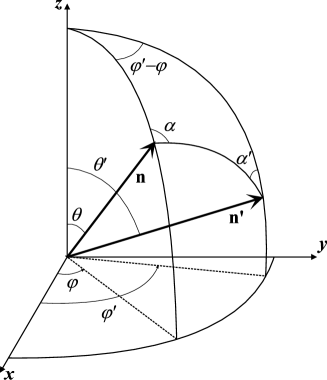
Figure 27: Definition of the angles and vectors for Thomson scattering in the general case. The polarization vectors are oriented like in figure 26.

To determine the cross section that a given ’initial’ wave
$(I^{(i)},Q^{(i)},U^{(i)})$ propagating in direction $n$ be scattered into a wave $(I^{(s)},Q^{(s)},U^{(s)})$ with direction $\mbox{\boldmath$n$}^{\prime}$, we need to go through the following steps (we will use the plane $({\mbox{\boldmath$y$}},{\mbox{\boldmath$z$}})$ as reference plane, see figure (27) for definitions of the angles and vectors):

1. Rotate around $n$ such that the plane $(\mbox{\boldmath$n$},\mbox{\boldmath$n$}^{\prime})$ turns into the plane $(\mbox{\boldmath$n$}{\mbox{\boldmath$z$}})$. One needs to apply the rotation (235,236) for $\phi=\alpha$ to the Stokes parameters.

2. Rotate the new plane $(\mbox{\boldmath$n$},\mbox{\boldmath$n$}^{\prime})$ around $z$ into the reference plane $({\mbox{\boldmath$y$}},{\mbox{\boldmath$z$}})$. This operation does not influence the incoming Stokes parameters..

3. Now we are in the known case of (233) and (234). Hence we can apply the scattering matrix.

4. We then rotate the scattering plane back around $z$ into the old $({\mbox{\boldmath$z$}},\mbox{\boldmath$n$}^{\prime})$ plane. This does not change the scattered Stokes parameters.

5. Finally we rotate around $\mbox{\boldmath$n$}^{\prime}$ by the angle $\alpha^{\prime}$ to reach the original state. To do this, we have to apply the rotation matrix (235,236) again, but now for $\phi=\alpha^{\prime}$.

Following the steps outlined above, we recover the scattering matrix in the basis $(I_{1},I_{2},U)$ given in equations (238) - (241) (see also [22]). $V$ is completely decoupled from the other parameters and follows an evolution which is independent of the rest. Hence by starting with $V(t\ll t_{dec})=0$ it will stay zero and can be neglected. The scattering matrix $P$, which determines the (non vanishing) scattered Stokes parameters from the initial ones,

$$\left(\begin{array}[]{c}I_{1}^{(s)}\\ I_{2}^{(s)}\\ U^{(s)}\end{array}\right)={\sigma_{T}\over 4\pi}P\left(\begin{array}[]{c}I_{1}^{(i)}\\ I_{2}^{(i)}\\ U^{(i)}\end{array}\right)$$ (237)

is then given by

$$P=\left[P^{(0)}+\sqrt{1-\mu^{2}}\sqrt{1-\mu^{\prime 2}}P^{(1)}+P^{(2)}\right],$$ (238)

where

$$P^{(0)}=\frac{3}{4}\left(\begin{array}[]{ccc}2(1-\mu^{2})(1-\mu^{\prime 2})+\mu^{2}\mu^{\prime 2}&\mu^{2}&0\\ \mu^{\prime 2}&1&0\\ 0&0&0\end{array}\right),$$ (239)

$$P^{(1)}=\frac{3}{4}\left(\begin{array}[]{ccc}4\mu\mu^{\prime}\cos(\phi^{\prime}-\phi)&0&2\mu\sin(\phi^{\prime}-\phi)\\ 0&0&0\\ -4\mu^{\prime}\sin(\phi^{\prime}-\phi)&0&2\cos(\phi^{\prime}-\phi)\end{array}\right),$$ (240)

$$P^{(2)}=\frac{3}{4}{\scriptsize\left(\begin{array}[]{ccc}\mu^{2}\mu^{\prime 2}\cos[2(\phi^{\prime}-\phi)]&-\mu^{2}\cos[2(\phi^{\prime}-\phi)]&\mu^{2}\mu^{\prime}\sin[2(\phi^{\prime}-\phi)]\\ -\mu^{\prime 2}\cos[2(\phi^{\prime}-\phi)]&\cos[2(\phi^{\prime}-\phi)]&-\mu^{\prime}\sin[2(\phi^{\prime}-\phi)]\\ -2\mu\mu^{\prime 2}\sin[2(\phi^{\prime}-\phi)]&2\mu\sin[2(\phi^{\prime}-\phi)]&2\mu\mu^{\prime}\cos[2(\phi^{\prime}-\phi)]\end{array}\right)}~{}.$$ (241)

As we are in an isotropic situation, we will perform all the calculations in a special coordinate system with $\mbox{\boldmath$k$}\parallel\hat{\mbox{\boldmath$z$}}$ and $\mbox{\boldmath$n$},\mbox{\boldmath$n$}^{\prime}$ as in Fig. 27. Clearly the results are independent of this coordinate choice.

The matrix $R$ connecting $(I_{1},I_{2},U)$ with $(I,Q,U)$ is given by

$$\left(\begin{array}[]{c}I_{1}\\ I_{2}\\ U\end{array}\right)=\left(\begin{array}[]{c}1/2(I+Q)\\ 1/2(I-Q)\\ U\end{array}\right)=\frac{1}{2}\left(\begin{array}[]{rrr}1&1&0\\ 1&-1&0\\ 0&0&2\end{array}\right)\left(\begin{array}[]{c}I\\ Q\\ U\end{array}\right)\equiv R\left(\begin{array}[]{c}I\\ Q\\ U\end{array}\right).$$ (242)

To calculate the collision term including polarization , we change into the $(I_{1},I_{2})$ basis. For each of the two intensities $\lambda\in\{1,2\}$ we then have the collision term given by

$$C[f^{(\lambda)}]=\frac{df_{+}^{(\lambda)}}{d\tau}-\frac{df_{-}^{(\lambda)}}{d\tau},$$ (243)

where $f_{+}^{(\lambda)}$ and $f_{-}^{(\lambda)}$ denote the distribution of photons in the polarization state $\lambda$ scattered into respectively out of the beam due to Thomson scattering.

In the matter (baryon/electron) rest frame, which we indicate by a prime, we know that

$${df_{+}^{(\lambda)\prime}\over dt^{\prime}}(p,\mbox{\boldmath$n$})={\sigma_{T}n_{e}\over 4\pi}\int P^{\lambda}_{~{}\delta}({\mbox{\boldmath$n$},\mbox{\boldmath$n$}}^{\prime})f^{(\delta)\prime}(p^{\prime},\mbox{\boldmath$n$}^{\prime})d\Omega^{\prime}\;,$$

where $n_{e}$ denotes the electron number density and $P^{\lambda}_{\delta}$ is the $2\times 2$ upper left corner of the normalized Thomson scattering matrix (238). In the baryon rest frame which moves with four velocity $u$, the photon energy is given by

$$p^{\prime}=p_{\mu}u^{\mu}\;.$$

We denote the photon energy with respect to a tetrad adapted to the slicing of space-time into $\{\tau=$ constant$\}$ hyper–surfaces by $p$ :

$$p=p_{\mu}n^{\mu}\;,~{}~{}~{}\mbox{ with }~{}~{}n=a^{-1}[(1-A)\partial_{\tau}+B^{i}\partial_{i}]~{},~{}$$

The lapse function and the shift vector of the slicing are given by $\alpha=a(1+A)$ and $\mbox{\boldmath$\beta$}=-B^{i}\partial_{i}$ . In first order,

$$p_{0}=ap(1+A)-apn_{i}B^{i}~{}~{},$$

and to zeroth order $p_{i}=apn_{i}$. Furthermore, the baryon four velocity has the form $u^{0}=a^{-1}(1-A)~{}~{},~{}~{}~{}u^{i}=u^{0}v^{i}$ up to first order. This yields

$$p^{\prime}=p_{\mu}u^{\mu}=p(1+n_{i}(v^{i}-B^{i}))\;.$$

Using this identity and performing the integration over photon energies, we obtain

$$\rho_{\gamma}{d\iota_{+}^{(\lambda)}(\mbox{\boldmath$n$})\over d\tau^{\prime}} = a\rho_{\gamma}\sigma_{T}n_{e}\left[1+4n_{i}(v^{i}-B^{i})+\right.$$

$$\left.{1\over 4\pi}\int\iota^{(\delta)}(\mbox{\boldmath$n$}^{\prime})P^{\lambda}_{\delta}(\mbox{\boldmath$n$},\mbox{\boldmath$n$}^{\prime})d\Omega^{\prime}\right]~{}.$$

Photons which are scattered leave the beam with the probability given by the Thomson cross section (see e.g.  [101])

$${df^{(\lambda)}_{-}\over dt^{\prime}}=\sigma_{T}n_{e}f^{(\lambda)\prime}(p^{\prime},\mbox{\boldmath$n$})~{},$$

so that we finally have

$$C^{(\lambda)\prime} = \frac{4\pi}{\rho_{\gamma}a^{4}}\int dp\left({df^{(\lambda)}_{+}\over dt^{\prime}}-{df^{(\lambda)}_{-}\over dt^{\prime}}\right)p^{3}=\frac{1}{2}\sigma_{T}n_{e}\big{[}4n_{i}(v^{i}-B^{i})-\iota^{(\lambda)}$$ (244)

$$~{}~{}~{}+{1\over 4\pi}\int\iota^{(\delta)}(\mbox{\boldmath$n$}^{\prime})P^{\lambda}_{\delta}({\mbox{\boldmath$n$},\mbox{\boldmath$n$}}^{\prime})d\Omega^{\prime}\big{]}~{}.$$

By setting $C^{({\cal M})}=C^{(1)}+C^{(2)}$ and $C^{(Q)}=C^{(1)}-C^{(2)}$ we transform the collision integral back to the normal stokes parameters. The term for $U$ has the same form as the one for $Q$, just with the corresponding matrix elements in the integral. The Boltzmann equation then finally becomes (setting ${\cal E}\equiv({\cal M},Q,U)$ and for the flat case, $\kappa=0$):

$$\dot{{\cal M}}+i\mu k{\cal M}=4i\mu k(\Phi-\Psi+n^{m}\Sigma^{(V)}_{m})+4n^{\ell}n^{m}\dot{H}_{m\ell}$$ (245)

$$+a\sigma_{T}n_{e}\left[-{\cal M}-4i\mu V_{b}+4n^{\ell}\omega_{b,\ell}+\int d\Omega^{\prime}P^{\alpha}_{1}{\cal E}^{\prime}_{\alpha}\right]$$

$$\dot{Q}+i\mu kQ=a\sigma_{T}n_{e}\left[-Q+\int d\Omega^{\prime}P^{\alpha}_{2}{\cal E}^{\prime}_{\alpha}\right]$$ (246)

$$\dot{U}+i\mu kU=a\sigma_{T}n_{e}\left[-U+\int d\Omega^{\prime}P^{\alpha}_{3}{\cal E}^{\prime}_{\alpha}\right]$$ , (247)

where we have to use the scattering matrix transformed into the $({\cal M},Q,U)$ basis,

$$P=P_{S}+P_{V}+P_{T}$$ (248)

with

$$P^{(S)} = R^{-1}P^{(0)}R$$ (249)

$$= \frac{3}{8}\left(\begin{array}[]{cc}3-\mu^{2}-\mu^{\prime 2}+3\mu^{2}\mu^{\prime 2}&(1-3\mu^{2})(1-\mu^{\prime 2})\\ (1-\mu^{2})(1-3\mu^{\prime 2}&3(1-\mu^{2})(1-\mu^{\prime 2})\end{array}\right)$$ (252)

$$P_{V} = \sqrt{1-\mu^{2}}\sqrt{1-\mu^{\prime 2}}R^{-1}P^{(1)}R$$ (253)

$$= \frac{3}{2}\sqrt{1-\mu^{2}}\sqrt{1-\mu^{\prime 2}}\left(\begin{array}[]{ccc}\mu\mu^{\prime}C&\mu\mu^{\prime}C&-\mu S\\ \mu\mu^{\prime}C&\mu\mu^{\prime}C&-\mu S\\ \mu^{\prime}S&\mu^{\prime}S&C\end{array}\right)$$ (257)

$$P_{T} = R^{-1}P^{(2)}R$$ (258)

$$= \frac{3}{8}\scriptsize{\left(\begin{array}[]{ccc}(1-\mu^{2})(1-\mu^{\prime 2})C_{T}&-(1-\mu^{2})(1+\mu^{\prime 2})C_{T}&2(1-\mu^{2})\mu^{\prime}S_{T}\\ -(1+\mu^{2})(1-\mu^{\prime 2})C_{T}&(1+\mu^{2})(1+\mu^{\prime 2})C_{T}&-2(1+\mu^{2})\mu^{\prime}S_{T}\\ -2\mu(1-\mu^{\prime 2})S_{T}&2\mu(1+\mu^{\prime 2})S_{T}&4\mu\mu^{\prime}C_{T}\end{array}\right)}$$ (262)

with $C=\cos(\phi-\phi^{\prime})$, $S=\sin(\phi-\phi^{\prime})$ and
$C_{T}=\cos(2(\phi-\phi^{\prime}))$, $S_{T}=\sin(2(\phi-\phi^{\prime}))$. The parts $P_{S},~{}P_{V},~{}P_{T}$ of $P$ describe the scattering of the scalar, vector and tensor contribution to ${\cal E}$ respectively.

The functions ${\cal M}$, $Q$ and $U$ depend on the wave vector $k$, the photon direction $n$ and conformal time $\tau$. We choose for each $k$-mode a reference system with $z$-axis parallel to $k$. For scalar perturbations we achieve in this way azimuthal symmetry — the right-hand side of the Boltzmann equation and therefore also the brightness ${\cal M}^{(S)}$ depend only on $\mu=(\hat{\mbox{\boldmath$k$}}\cdot\mbox{\boldmath$n$})$ and can be expanded in Legendre polynomials. The right-hand side of the Boltzmann equation also determines the azimuthal dependence of vector and tensor perturbations. One can continue with this approach, but the resulting equations for $Q$ and $U$ and especially also their power spectra depend explicitly on the coordinate system. Therefore, we prefer an approach which is inherently covariant under rotation.

B.3 Electric and magnetic polarization

Since the Stokes parameters explicitly depend on the coordinate system, and Eqs. (246) and (247) transform in a rather complicated way under rotations of the coordinate system. A method to characterize CMB polarization due to non-relativistic Thomson scattering, which is more convenient than the Stokes parameters since its transformation properties are very simple, has been developed a couple years ago [130, 162, 84, 85, 72]. A detailed derivation of this method goes beyond the scope of this report. Here we just repeat the definitions and the main results. We set

$$\mbox{\boldmath$\cal T$}=({\cal M},Q+iU,Q-iU)$$ (263)

In terms of this three component vector the collision integral above can we written (in vector form) as

$$\mbox{\boldmath$C$}[\mbox{\boldmath$\cal T$}] = a\sigma_{T}n_{e}[-\mbox{\boldmath$\cal T$}+\left({1\over 4\pi}\int\d\Omega^{\prime}{\cal M}^{\prime}+(\mbox{\boldmath$n$}\cdot{\bf v}_{b}),0,0\right)$$ (264)

$$+{1\over 10}\sum_{m=-2}^{2}\int\d\Omega^{\prime}P^{(m)}(\mbox{\boldmath$n$},\mbox{\boldmath$n$}^{\prime})\mbox{\boldmath$\cal T$}^{\prime}$$

From Eqs. (238) to (242) one can determine the scattering matrix for the vector $\cal T$

$$P^{(m)}=\left(\begin{array}[]{ccc}Y_{2}^{m^{\prime}}Y_{2}^{m}&-\sqrt{{3\over 2}}{{}_{2}Y_{2}^{m^{\prime}}}Y_{2}^{m}&-\sqrt{{3\over 2}}_{-2}Y_{2}^{m^{\prime}}Y_{2}^{m}\\ -\sqrt{6}Y_{2}^{m^{\prime}}{{}_{2}Y_{2}^{m}}&3_{2}Y_{2}^{m^{\prime}}{{}_{2}Y_{2}^{m}}&3_{-2}Y_{2}^{m^{\prime}}{{}_{2}Y_{2}^{m}}\\ -\sqrt{6}Y_{2}^{m^{\prime}}{{}_{-2}Y_{2}^{m}}&3_{2}Y_{2}^{m^{\prime}}{{}_{-2}Y_{2}^{m}}&3_{-2}Y_{2}^{m^{\prime}}{{}_{-2}Y_{2}^{m}}\end{array}\right)$$ (265)

where ${}_{s}Y_{l}^{m^{\prime}}={{}_{s}Y_{l}^{m*}(\mbox{\boldmath$n$}^{\prime})}$ and ${}_{s}Y_{l}^{m}={{}_{s}Y_{l}^{m*}}(\mbox{\boldmath$n$})$ are the spin-weighted spherical harmonics [111, 85, 76].

We now decompose the Fourier components of the temperature anisotropy ${\cal M}$ and the polarization variables $Q$ and $U$ as

$${\cal M} = \sum_{\ell}\sum_{m=-2}^{2}{\cal M}_{\ell}^{(m)}{{}_{0}G^{m}_{\ell}},$$ (266)

$$Q\pm iU = \sum_{\ell}\sum_{m=-2}^{2}(E_{\ell}^{(m)}\pm iB_{\ell}^{(m)}){{}_{2}G^{m}_{\ell}}(\mbox{\boldmath$n$}).$$ (267)

Here $m=0$ is the scalar mode, $m=\pm 1$ are the vector and $m=\pm 2$ are the tensor modes. The functions ${}_{s}G^{m}_{\ell}$ are closely related to the spin weighted harmonics ${}_{s}Y^{m}_{\ell}$:

$${}_{s}G^{m}_{\ell}(\mbox{\boldmath$n$})=(-i)^{\ell}\sqrt{{4\pi\over 2\ell+1}}{{}_{s}Y^{m}_{\ell}}(\mbox{\boldmath$n$})$$

The evolution equations in term of these variables can be given in the following compact form [72]

$$\dot{\cal M}_{\ell}^{(m)}-k\left[{{}_{0}\kappa^{m}_{\ell}\over 2\ell-1}{\cal M}_{\ell-1}^{(m)}-{{}_{0}\kappa^{m}_{\ell+1}\over 2\ell+3}{\cal M}_{\ell+1}^{(m)}\right]=$$ (268)

$$-n_{e}\sigma_{T}a{\cal M}_{\ell}^{(m)}+S_{\ell}^{(m)}~{}~{}~{}(\ell\geq m)$$

$$\dot{E}_{\ell}^{(m)}-k\left[{{}_{2}\kappa^{m}_{\ell}\over 2\ell-1}E_{\ell-1}^{(m)}-{2m\over\ell(\ell+1)}B_{\ell}^{(m)}-{{}_{2}\kappa^{m}_{\ell+1}\over 2\ell+3}E_{\ell+1}^{(m)}\right]=$$ (269)

$$-n_{e}\sigma_{T}a[E_{\ell}^{(m)}+\sqrt{6}C^{(m)}\delta_{\ell,2}]~{}~{}~{}(\ell\geq 2)$$

$$\dot{B}_{\ell}^{(m)}-k\left[{{}_{2}\kappa^{m}_{\ell}\over 2\ell-1}B_{\ell-1}^{(m)}+{2m\over\ell(\ell+1)}E_{\ell}^{(m)}-{{}_{2}\kappa^{m}_{\ell+1}\over 2\ell+3}B_{\ell+1}^{(m)}\right]=$$ (270)

$$-n_{e}\sigma_{T}aB_{\ell}^{(m)}~{}~{}~{}(\ell\geq 2)~{}.$$

where we have set

$$\begin{array}[]{cc}S_{0}^{(0)}=n_{e}\sigma_{T}a{\cal M}^{(0)}_{0},&S^{(0)}_{1}=n_{e}\sigma_{T}a4V_{b}+4k(\Psi-\Phi),\\ S^{(0)}_{2}=n_{e}\sigma_{T}aC^{(0)},&S^{(1)}_{1}=n_{e}\sigma_{T}a4\sqrt{2}\omega_{b},\\ S^{(1)}_{2}=n_{e}\sigma_{T}aC^{(1)}+4\sqrt{2/3}k\Sigma,&S^{(2)}_{2}=n_{e}\sigma_{T}aC^{(2)}-8\sqrt{2/3}\dot{H}\end{array}$$

and $C^{(m)}={1\over 10}[{\cal M}^{(m)}_{2}-\sqrt{6}E^{(m)}_{2}]$. The coupling coefficients are

$${}_{s}\kappa^{m}_{\ell}=\sqrt{{(\ell^{2}-m^{2})(\ell^{2}-s^{2})\over\ell^{2}}}.$$

Note that for scalar perturbations, $m=0$, $B$-polarization is not sourced and we have $B_{\ell}^{(0)}\equiv 0$.

Finally, we want to connect the intensities ${\cal M}^{(m)}_{\ell}$ with the more familiar expansion of the scalar $(S)$, vector $(V)$ and tensor $(T)$ contributions to the brightness function in terms of Legendre polynomials. Usually one sets

$${\cal M}={\cal M}^{(S)}+{\cal M}^{(V)}+{\cal M}^{(T)}~{}.$$

Here ${\cal M}^{(S)}$ only depends on $\mu=(\mbox{\boldmath$n$}\cdot\mbox{\boldmath$k$})/k$ and the $n$-dependence of ${\cal M}^{(V)}$ and ${\cal M}^{(T)}$ can be written as

$${\cal M}^{(V)}(\mu,\phi) = \sqrt{1\!-\!\mu^{2}}\left[{\cal M}_{1}^{(V)}(\mu)\cos\phi\!+\!{\cal M}_{2}^{(V)}(\mu)\sin\phi\right]$$ (271)

$${\cal M}^{(T)}(\mu,\phi) = (1-\mu^{2})\left[{\cal M}_{+}^{(T)}\cos(2\phi)+{\cal M}_{\times}^{(T)}\sin(2\phi)\right],$$ (272)

where $\phi$ is the azimuthal angle in the plane normal to $k$. Each of the functions ${\cal M}_{\bullet}^{(S,V,T)}(\mu)$ is now expanded in Legendre polynomials

$${\cal M}_{\bullet}^{(S,V,T)}=\sum_{\ell}(-i)^{\ell}(2\ell+1)\sigma_{\bullet,\ell}^{(S,V,T)}P_{\ell}(\mu)~{}.$$ (273)

The coefficients $\sigma_{\bullet,\ell}^{(S,V,T)}$ are then related to ${\cal M}_{\ell}^{(m)}$ via the identities

$${\cal M}_{\ell}^{(0)} = (2\ell+1)\sigma_{\ell}^{(S)}$$ (274)

$${\cal M}_{\ell}^{(\pm 1)} = \sqrt{\ell(\ell+1)}\left[\left(\sigma^{(V)}_{2,\ell-1}+\sigma^{(V)}_{2,\ell+1}\right)\right.$$ (275)

$$~{}~{}~{}\left.\pm i\left(\sigma^{(V)}_{1,\ell-1}+\sigma^{(V)}_{1,\ell+1}\right)\right]$$

$${\cal M}_{\ell}^{(\pm 2)} = -\sqrt{(\ell+2)!\over(\ell-2)!}\left[{1\over 2\ell+3}\sigma_{\uparrow\downarrow,\ell+2}^{(T)}+{2(2\ell+1)\over(2\ell-1)(2\ell+3)}\sigma_{\uparrow\downarrow,\ell}^{(T)}\right.$$

$$~{}~{}~{}\left.+{1\over 2\ell-1}\sigma_{\uparrow\downarrow,\ell-2}^{(T)}\right]$$

$$\mbox{ with }\sigma_{\uparrow\downarrow,\ell}^{(T)}=\sigma_{+,\ell}^{(T)}\mp i\sigma_{\times,\ell}^{(T)}$$

We do not repeat this correspondence for the Stokes parameters $Q$ and $U$ since it is rather complicated and not very useful as it depends on the coordinate system chosen.

B.4 Power spectra

Since they are functions on a sphere, the observed CMB anisotropies and polarization are conveniently expanded in spherical harmonics: $\delta T(\mbox{\boldmath$n$},\tau_{0})/T_{0}=\sum_{\ell m}a_{\ell m}Y_{\ell}^{m}(\mbox{\boldmath$n$})$. The coefficients $a_{\ell m}$ are random variables with zero mean and rotationally invariant variances, $C_{\ell}\equiv\langle\mid a_{\ell m}\mid^{2}\rangle$. The correlation function of the anisotropy pattern then has the standard expression:

$$\left\langle{\delta T\over T_{0}}(\mbox{\boldmath$n$}_{1}){\delta T\over T_{0}}(\mbox{\boldmath$n$}_{2})\right\rangle={1\over 4\pi}\sum_{\ell}(2\ell+1){C_{\ell}}P_{\ell}(\cos\theta)$$ (277)

where $\cos\theta=\mbox{\boldmath$n$}_{1}\cdot\mbox{\boldmath$n$}_{2}$ and $\langle\cdots\rangle$ denotes ensemble average. We use the Fourier transform normalization

$$\hat{f}(\mbox{\boldmath$k$})={1\over V}\int f({\bf x})\exp(i\mbox{\boldmath$k$}\cdot{\bf x})d^{3}x~{},$$ (278)

with some normalization volume $V$. Using statistical homogeneity we have

$$\left\langle{\delta T\over T_{0}}(\mbox{\boldmath$n$}_{1}){\delta T\over T_{0}}(\mbox{\boldmath$n$}_{2})\right\rangle={1\over V}\int d^{3}x\left\langle{\delta T\over T_{0}}({\bf x},\mbox{\boldmath$n$}_{1}){\delta T\over T_{0}}({\bf x},\mbox{\boldmath$n$}_{2})\right\rangle$$ (279)

$$= {1\over(2\pi)^{3}}\int d^{3}k\left\langle{\delta T\over T_{0}}(\mbox{\boldmath$k$},\mbox{\boldmath$n$}_{1}){\delta T\over T_{0}}(\mbox{\boldmath$k$},\mbox{\boldmath$n$}_{2}\right\rangle)~{}.$$

Inserting our ansatz (273) for ${\delta T\over T_{0}}={1\over 4}{\cal M}$, and using the addition theorem for spherical harmonics,
$P_{\ell}(\mbox{\boldmath$n$}_{1}\cdot\mbox{\boldmath$n$}_{2})=\frac{4\pi}{2\ell+1}\sum_{m}Y_{\ell m}^{*}(\mbox{\boldmath$n$}_{1})Y_{\ell m}(\mbox{\boldmath$n$}_{2})$, we find

$$\left\langle{\delta T\over T_{0}}(\mbox{\boldmath$n$}_{1}){\delta T\over T_{0}}(\mbox{\boldmath$n$}_{2})\right\rangle={1\over 8\pi}\sum_{\ell,\ell^{\prime},m,m^{\prime}}(-1)^{(\ell-\ell^{\prime})}Y_{\ell m}(n_{1})Y^{*}_{\ell^{\prime}m^{\prime}}(n_{2})$$

$$\times\int k^{2}dkd\Omega_{\hat{\mbox{\boldmath$k$}}}Y_{\ell m}^{*}(\hat{\mbox{\boldmath$k$}})Y_{\ell^{\prime}m^{\prime}}(\hat{\mbox{\boldmath$k$}})\langle\sigma_{\ell}\sigma^{*}_{\ell^{\prime}}\rangle(k)$$

$$= {1\over 32\pi^{2}}\sum_{\ell}(2\ell+1)P_{\ell}(\mbox{\boldmath$n$}_{1}\cdot\mbox{\boldmath$n$}_{2})\int k^{2}dk\langle\sigma_{\ell}\sigma^{*}_{\ell}\rangle(k)~{},$$ (280)

from which we conclude

$$C_{\ell}^{{\cal M}{\cal M},(S)}={1\over{8\pi}}\int k^{2}dk\langle|\sigma^{(S)}_{\ell}(t_{0},k)|^{2}\rangle~{},$$ (281)

where the superscript ^(S) indicates that Eq. (281) gives the contribution from scalar perturbations and ^MM means that it is the contribution to the intensity perturbation.

The $QQ$, $UU$, ${\cal M}Q$, ${\cal M}U$ and $QU$ correlators depend with the Stokes parameters on the particular coordinate system chosen. It is much more convenient to express the polarization power spectra in terms of the variables $E$ and $B$ which are independent of the coordinate system. Furthermore, since $B$ is parity odd, its correlators with ${\cal M}$ and $E$ vanish. One finds the simple general expression [72]

$$(2\ell+1)^{2}C_{\ell}^{XY(m)}={n_{m}\over 8\pi}\int k^{2}dkX_{\ell}^{(m)}Y_{\ell}^{(m)*}~{},$$ (282)

where $n_{m}=1$ for $m=0$ and $n_{m}=2$ for $m=1,2$, accounting for the number of modes. Here $X$ and $Y$ run over ${\cal M}$, $E$ and $B$.

References

- [1] A. Achúcarro and J. Urrestilla, Phys. Rev. Lett. 85 (2000) 3091.
- [2] A. Albrecht, R. Battye and J. Robinson, Phys. Rev. Lett. 79 (1997) 4736.
- [3] A. Albrecht, D. Coulson, P.G. Ferreira and J. Magueijo, Phys. Rev. Lett. 76 1413 (1996).
- [4] B. Allen et al., Phys. Rev. Lett 77 3061 (1996).
- [5] B. Allen et al., Phys. Rev. Lett. 79 (1997) 2624.
- [6] P.P. Avelino and C.J.A.P. Martins, preprint astro-ph/016303 (2001).
- [7] P.P. Avelino, E.P.S. Shellard, J.H.P. Wu and B. Allen, Phys. Rev. Lett. 81 (1998) 2008.
- [8] J. Bardeen, Phys. Rev. D22 (1980) 1882.
- [9] R.A. Battye, M. Bucher and D. Spergel, preprint astro-ph/9908047 (1999); M. Bucher and D. Spergel, Phys. Rev. D60 (1999) 043505.
- [10] C.M. Baugh and G. Efstathiou, M.N.R.A.S., 265 (1993) 145.
- [11] M.L. Bellac, Thermal Field Theory, Cambridge University Press (1996).
- [12] V. Berezinsky, B. Hnatyk and A. Vilenkin, preprint astro-ph/0102366 (2001).
- [13] V. Berezinsky, X. Martin and A. Vilenkin, Phys. Rev. D56 (1997) 2024.
- [14] F. Bernardeau and J.P. Uzan, Phys.Rev. D63 023005 (2001).
- [15] S. Bonazzola and P. Peter Astropart. Phys. 7 (1997) 161.
- [16] R. Bond & G. Efstathiou, Mon. Not. Roy. Ast. Soc., 304 (1998) 75.
- [17] Borill, J. et al. Phys. Rev. D50 (1994) 2469, and references therein.
- [18] M. Bucher and D. Spergel, Phys.Rev. D60 (1999) 043505
- [19] F. Bouchet, P. Peter, A. Riazuelo and M. Sakellariadou, preprint astro-ph/0005022 (1999).
- [20] B. Carter, A.C. Davis, Phys.Rev. D61 (2000) 123501.
- [21] B. Carter and P. Peter, Phys.Lett. B466, 41 (1999)
- [22] S. Chandrasekhar, Radiative Transfer, Oxford University Press (1950).
- [23] C. Cheung and J. Magueijo, Phys. Rev. D 56 (1997) 1982.
- [24] I. Chuang, R. Durrer, N. Turok and B. Yurke, Science 251 (1991) 1336.
- [25] S. Coleman and E. Weinberg, Phys. Rev. D7 (1973) 1887.
- [26] C. Contaldi, M. Hindmarsh and J. Magueijo, Phys. Rev. Lett. 82 (1999) 679.
- [27] C. Contaldi, M. Hindmarsh and J. Magueijo, Phys. Rev. Lett. 82 (1999) 2034.
- [28] R. Crittenden and N. Turok, Phys. Rev. Lett. 75 (1995) 2642.
- [29] L.N. Da Costa, M.S. Vogeley, M.J. Geller, J.P. Huchra and C. Park, Astrophys. J. 437 (1994) 1L.
- [30] D. Coulson, R.G.Crittenden and N.G. Turok, Phys. Rev. Lett. 73 (1994) 2390.
- [31] R.G. Crittenden, D. Coulson and N.G. Turok, Phys. Rev. D52 (1995) 5402.
- [32] A.C. Davis and M. Majumdar, 46.Phys.Lett. B460 (1999) 257
- [33] A.C. Davis and W.B. Perkins Phys. Lett. B393 (1997)
- [34] P. de Bernardis, A. Balbi, G. De Gasperis, A. Melchiorri and N. Vittorio, Astrophys. J. 480 (1997) 1.
- [35] P. de Bernardis et al., Nature 404 (2000) 955; preprint astro-ph/0004404.
- [36] A. Dekel, Ann. Rev. of Astron. and Astrophys. 32 (1994) 371.
- [37] J. Derrick, Math. Phys. 5 (1964) 1252 (1964).
- [38] N. Deruelle, D. Langlois and J.P. Uzan. Phys. Rev. D56 (1997) 7608, erratum ibid. D58 (1998) 089901.
- [39] L. Dolan and R. Jackiw, Phys. Rev. D9 (1974) 3320.
- [40] R. Durrer, Nucl. Phys. B328, 238 (1989).
- [41] R. Durrer, Phys. Rev. D42 (1990) 2533.
- [42] R. Durrer, Fund. of Cosmic Physics 15 (1994) 209.
- [43] R. Durrer, R. Juszkiewicz, M. Kunz and J.P. Uzan, Phys. Rev. D62 (2000) 021301(R).
- [44] R. Durrer, A. Gangui and M. Sakellariadou, Phys. Rev. Lett. 76 (1996) 579.
- [45] R. Durrer and M. Kunz, Phys. Rev. D57 (1998) R3199.
- [46] R. Durrer, M. Kunz, C. Lineweaver and M. Sakellariadou, Phys. Rev. Lett. 79 (1997) 5198.
- [47] R. Durrer, M. Kunz and A. Melchiorri, Phys. Rev. D59 (1999) 123005.
- [48] R. Durrer, M. Kunz and A. Melchiorri, Phys. Rev. D63 (2001) 081301(R).
- [49] R. Durrer and M. Sakellariadou, Phys. Rev. D56 (1997) 4480.
- [50] R. Durrer and N. Straumann, Helv. Phys. Acta 61 (1988) 1027.
- [51] R. Durrer and Z. Zhou, Phys. Rev. D53 (1996) 5394.
- [52] V.R. Eke, S. Cole and C.S. Frenk M.N.R.A.S. 282 (1996) 263E.
- [53] K. Enqvist, H. Kurki-Suonio and J. Valiviita; Phys.Rev. D62 (2000) 103003.
- [54] P. G. Ferreira and J. Magueijo, Phys. Rev. D55 (1997) 3358.
- [55] J. Filipe and A. Bray, Phys. Rev. E50 (1994) 2523
- [56] K.B. Fisher, M. Davis, M.A. Strauss, A. Yahil and J.P. Huchra, M.N.R.A.S. 266 (1994) 50.
-
[57]
W. Freedman, J.R. Mould, R.C. Kennicut and B.F. Madore,in:
Cosmological Parameters and the Evolution of the Universe,
K. Sato. edt. (Dordrecht, Boston: Kluwer Academic, 1999) 17.
preprint astro-ph/9801080 (1998). - [58] J. Fry, Astrophys. J. 279 (1984) 499.
- [59] A. Gangui, L. Pogosian and S. Winitzki, Phys. Rev. D64, 043001 (2001).
- [60] E. Gaztañaga and P. Mähönen, Astrophys. J. 462 (1996) L1.
- [61] T. Gherghetta, E. Roessl and M. Shaposhnikov, Phys. Lett. B491 (2000) 353.
- [62] T. Gherghetta and M. Shaposhnikov, Phys. Rev. Lett. 85 (2000) 240.
- [63] R. Giovanelli et al., preprint astro-ph/9807274 (1998).
- [64] J. Goldstone, Nuovo Cim. 19 (1961) 154.
- [65] R. Gregory, Phys. Rev. Lett. 84 2564 (2000), hep-th/9911015.
- [66] N.W. Halverson et al., preprint astro-ph/0104489 (200
- [67] A. J. Hamilton, M. Tegmark, M.N.R.A.S. L51 (2000) 276.
- [68] S. Hanany et al., Astrophys. J. Lett. 545, L5 (2000); preprint astro-ph/0005123 (2000).
- [69] E. Harrison, Phys. Rev. D1 (1970) 2726.
- [70] M. Hindmarsh, Nucl.Phys.Proc.Suppl. 43 (1995) 50.
- [71] M.B. Hindmarsh and T.W.B. Kibble, Rept. Prog. Phys. 58, (1995) 477.
- [72] W. Hu et al., Phys. Rev. D57 (1998) 3290.
- [73] W. Hu, D.N. Spergel and M. White, Phys. Rev. D 55 (1997) 3288.
- [74] W. Hu and N. Sugiyama, Phys. Rev. D 51 (1995) 2599, and references therein.
- [75] W. Hu, N. Sugiyama and J. Silk, Nature 386 (1995) 37.
- [76] W. Hu and M. White, Phys. Rev. D 56 (1997) 596.
- [77] Itzykson, C. and Zuber, J.B. Quantum Field Theory, (McGraw Hill, New York, 1980).
- [78] Jackson Classical Electrodynamics, Wiley & Sons, New York (1965).
- [79] R. Jeannerot, Phys.Rev. D56 (1997) 6205.
- [80] B.J. Jones and R. Wyse, Astron. & Astrophys. 149 (1985) 144.
- [81] N. Kaiser, Astrophys. J. 284 (1984) 9L.
- [82] N. Kaiser, G. Efstathiou, R. Ellis, C.S. Frenk, A. Lawrence, M. Rowan-Robinson and W. Saunders, M.N.R.A.S. 252 (1991) 1.
- [83] N. Kaiser and A. Stebbins, Nature 310 (1984) 391.
- [84] M. Kamionkowski, A. Kosowsky and A. Stebbins, Phys. Rev. Lett. 78 (1997) 2058.
- [85] M. Kamionkowski, A. Kosowsky and A. Stebbins, Phys. Rev. D55 (1997) 7368.
- [86] Kaputsa, J. I., Finite Temperature Field Theory, Cambridge University Press (1989).
- [87] S. Kasuya and M. Kawasaki, Phys.Rev. D61 (2000) 083510.
- [88] T.W.B. Kibble, Journal of Physics A9 (1976) 1387.
- [89] T.W.B. Kibble, Phys. Rep. 67 (1980) 183.
- [90] D.A. Kirzhnits and A. Linde, Phys. Lett. B42 (1972) 471.
- [91] H. Kodama and M. Sasaki, Prog. Theor. Phys. Suppl. 78 (1984) 1.
- [92] E. Kolb and M. Turner,. The Early Universe, (Addison-Wesley Publ. Comp., Redwood City, 1990).
- [93] A. Kosowsky, Annals of Physics 246 (1996) 49.
- [94] M. Kunz, Anisotropies in the Cosmic Microwave Background from Causal Scaling Seeds: Methods and Results, PhD Dissertation, University of Geneva (1999).
- [95] M. Kunz and R. Durrer, Phys. Rev. D 55 (1997) R4516.
- [96] A. Laix, L.M. Krauss and T. Vachaspati, Phys. Rev. Lett. 79, 1968 (1997).
- [97] A.T. Lee et al., preprint astro-ph/0104459 (2001).
- [98] L. Lichtsteiger and R. Durrer, Phys. Rev. D59 (1999) 125007.
- [99] A.R. Liddle, D. Lyth, H. Robeerts, P. Viana, M.N.R.A.S. 278 (1996) 644.
- [100] E. Lifshitz, ZhEFT 16, 587; J. Phys. USSR 10 (1946) 116.
- [101] E.M. Lifshitz and L.P. Pitajewski, Lehrbuch der Theoretischen Physik, Band X, Akademie Verlag Berlin (1983).
- [102] H. Lin et al., AAS 185 (1994) 5608L.
- [103] X. Luo, Astrophys. J. 439 (1995) 517L.
- [104] C.P. Ma and E. Bertschinger, Astrophys. J. 455 (1995) 7.
- [105] J. Magueijo, A. Albrecht, P.G. Ferreira and D. Coulson, Phys. Rev. D 54 (1996) 3727.
- [106] J. Magueijo and R. Brandenberger in:Large Scale Structure Formation”, Kluwer (Dortrecht 2000).
- [107] A. Melchiorri and N. Vittorio, in: Proceedings of the NATO Advanced Study Institute 1996 on the ”Cosmic Background Radiation”, Strasbourg, archived under astro-ph/9610029, (1996).
- [108] A. Melott and R. Scherrer, Nature 328 (1987) 691.
- [109] N.D. Mermin, Rev. Mod. Phys. 51 (1979) 591.
- [110] C.B. Netterfield et al., preprint astro-ph/0104460, (2001).
- [111] E. Newman and R. Penrose, J. Math. Phys. 7 (1966) 863.
- [112] H. Nielsen and P. Olesen, Nucl. Phys. B81 (1973) 45.
- [113] T. Padmanabhan, Structure formation in the universe, Cambridge University Press (1993).
- [114] J.A. Peacock, M.N.R.A.S. 284 (1997) 885P.
- [115] P.J.E. Peebles, Principles of Physical Cosmology, Princeton University Press (1993).
- [116] P.J.E. Peebles and J.T. Yu, Astrophys. J. 162 (1970) 815
- [117] U. Pen, U. Seljak and N. Turok, Phys. Rev. Lett. 79 (1997) 1611.
- [118] U. Pen, D. Spergel and N. Turok, Phys Rev. D 49 (1994) 692.
- [119] W.P. Petersen and A. Bernasconi, CSCS Technical Report TR-97-06 (1997).
- [120] E. Pierpaoli, J. Garcia-Bellido and S. Borgani, Astrophys. J. Lett. 505 (1999) L91.
- [121] L. Pogosian and T. Vachaspati, Phys. Rev. D60 (1999) 083504.
- [122] A.M. Polyakov, JETP Lett. 20, 194 (1974); G. ’t Hooft, Nucl. Phys. B79 (1974) 276.
- [123] M.K. Pradas and C.M. Sommerfeld, Phys. Rev. Lett. 35 (1975) 760.
- [124] A. Riazuelo, N. Deruelle and P. Peter Phys.Rev. D61 (2000) 123504.
- [125] A. Riess et al. AJ, 116 (1998) 1009; S. Perlmutter et al., Astrophys. J. 517 (1999) 565.
- [126] K. Rummukainen, M. Tsypin, K. Kajantie, M. Laine and M. Shaposhnikov, Nucl. Phys. B532 (1998) 283.
- [127] M. Sakellariadou and A. Vilenkin, Phys. Rev. D 42, (1990) 349.
- [128] U. Seljak, U. Pen and N. Turok, Phys. Rev. Lett. 79 (1997) 1615.
- [129] U. Seljak and M. Zaldarriaga, Astrophys. J. 496 (1996) 437.
- [130] U. Seljak and M. Zaldarriaga, Phys. Rev. Lett., 78, 2054 (1997).
- [131] E.J. Shaia, P.J.E. Peebles and R.B. Tully, Astrophys. J. 454 (1995) 15.
- [132] P. Shellard, private communication (1998).
- [133] A.G. Smith and A. Vilenkin, Phys. Rev. D 36 (1987) 990.
- [134] G. Smoot, et al., Astrophys. J. 396 (1992) L1.
- [135] D. Spergel & M. Zaldarriaga, Phys. Rev. Lett. 79 (1997) 2180.
- [136] D. Spergel, and U. Pen, Astrophys. J 491 (1997) L67.
- [137] V. Springel, R. Juszkiewicz and R. Durrer, Astrophys. J. Lett. 518 (1999) L25.
- [138] D.A. Steer, Phys.Rev. D63 083517 (2001).
- [139] J.M. Stewart, Non-Equilibrium Relativistic Kinetic Theory, Springer Lecture Notes in Physics, Vol. 10, ed. J. Ehlers, K. Hepp and H.A. Wienmüller (1971).
- [140] J.M. Stewart and M. Walker, Proc. R. Soc. London A341 (1974) 49.
- [141] W. Sutherland et al., M.N.R.A.S., 381 (1999) 459.
- [142] H. Tadros and G. Efstathiou, M.N.R.A.S. L45 (1995) 276.
- [143] N. Turok, Phys. Rev. D54 (1996) R3686.
- [144] N. Turok, Phys. Lett. 77 (1996) 4138.
- [145] N. Turok and D. Spergel, Phys. Rev. Lett. 64 (1990) 2736.
- [146] N. Turok and D. Spergel, Phys. Rev. Lett 66 (1991) 3093.
- [147] J.P. Uzan, Class. Quant. Grav. 15 (1998) 1063.
- [148] J.P. Uzan and F. Bernardeau, Phys.Rev. D63 (2001) 023004.
- [149] J.P. Uzan, N. Deruelle and N. Turok, Phys. Rev. D57, (1998) 7192.
- [150] S. Veeraraghavan & A. Stebbins, Astrophys. J. 365 (1990) 37.
- [151] T. Vachaspati and A. Vilenkin, Phys. Rev. D31 (1985) 3052.
- [152] A. Vilenkin and E.P.S. Shellard, Cosmic Strings and other Topological Defects Cambridge University Press (1995).
- [153] G.R. Vincent, M. Hindmarsh and M. Sakellariadou, Phys. Rev. D56 (1997) 637.
- [154] G.R. Vincent, N. Antunes and M. Hindmarsh, Phys.Rev. Lett. 80 (1998) 2277.
- [155] M.S. Vogeley, to appear in ”Ringberg Workshop on Large-Scale Structure”, ed. D. Hamilton, (Kluwer, Amsterdam), archived under astro-ph/9805160 (1998).
- [156] S. Weinberg, Phys. Rev. D9, 3357 (1974).
- [157] S. Weinberg, Field Theory, Vol. 2, Cambridge University Press (1996).
- [158] J.A. Willick, S. Courteau, S.M. Faber, D. Burstein, A. Dekel and T. Kolatt, Astrophys. J. 457 (1996) 460.
- [159] E. Witten, Nucl. Phys B249 (1985) 557.
- [160] J.H.P. Wu et al., DAMTP-1998-161, archived under astro-ph/9812156
- [161] J. H. Wu et al., preprint astro-ph/0104248. (2001).
- [162] M. Zaldarriaga and U. Seljak, Phys. Rev. D55 (1997) 1830.
- [163] Ya.B. Zel’dovich, Mont. Not. R. Astr. Soc. 160 (1972) P1.
- [164] W. Zurek, Nature 317, 505 (1985); W. Zurek, Phys. Rep. 276 (1996) 177.
-
[165]
See the following web sites for information about the Planck
and MAP satellite projects:
http://astro.estec.esa.nl/SA-general/Projects/Planck/
and http://map.gsfc.nasa.gov/ -
[166]
Information about RADpack can be found on the homepage
of L. Knox:
http://bubba.ucdavis.edu/ knox/radpack.html