Redshift of reionization: are we there yet?

Abstract

Comparison of the observed evolution of the Ly-alpha transmitted flux in the spectra of four highest redshift quasars discovered by SLOAN survey with the theoretical prediction for this evolution based on the state-of-the-art numerical simulations of cosmological reionization already allows one to constrain the redshift of reionization to $z_{\rm REI}=6.2\pm 0.1{\rm s}\pm 0.2{\rm r}$, where systematic and random errors are given respectively.

1 Introduction

In a recent paper Becker et al. [Becker et al. 2001] analysed spectra of the four highest redshift quasars discovered by SLOAN survey. The highest redshift ($z=6.28$) quasar showed almost no transmitted flux just blueward of the quasar Ly-alpha emission line, and on this bases Becker et al. [Becker et al. 2001] concluded that reionization took place at a redshift $z\sim 6$ [a similar claim was also made by Djorgovski et al. [Djorgovski et al. 2001] based on an extrapolation from a lower redshift observations].

However, one should be cautious before drawing such a conclusion. Indeed, the observed decrease in the mean transmitted flux at $z\sim 6$ might simply indicate a decrease in the mean ionizing intensity rather then a real reionization of the universe. Thus, without an understanding of the evolution of the universe around the reionization epoch, the Ly-alpha absorption data cannot be used to constrain the epoch of reionization [unless damping wings are observed in the absorption profiles, [Miralda-Escudé 1998]].

Fortunately, our theoretical understanding of the process of reionization, in part based on numerical simulations, is solid enough so that the evolution of the ionizing intensity at these redshifts can be predicted with a reasonable confidence level. Combining simulations with the observational data indeed allows one to come up with a meaningful value for the redshift of reionization.

2 Simulations

A set of three simulations have been performed with the SLH code and are similar to the simulations reported in [Gnedin 2000a]. The main difference with previous simulations is that a newly developed and highly accurate Optically Thin Eddington Variable Tensor (OTVET) approximation for modeling radiative transfer [Gnedin & Abel 2001] is used instead of a crude Local Optical Depth approximation. The new simulations therefore should be sufficiently accurate (subject to the usual limitations of numerical convergence and phenomenological description of star formation) to be used meaningfully in comparing with the observational data.

Table 1: Simulation Parameters

Run	$\Omega_{m,0}$	$n$	$z_{\rm REI}$	$\epsilon_{\rm SF}$	$\epsilon_{\rm UV}/(4\pi)$
A	0.30	1.0	6.70	0.20	$3\times 10^{-6}$
B	0.35	0.95	5.90	0.15	$6\times 10^{-6}$
C	0.35	0.97	5.95	0.15	$2.5\times 10^{-6}$

Parameters of the three simulations are given in Table 1. All three simulations included $64^{3}$ dark matter particles, an equal number of baryonic cells on a quasi-Lagrangian moving mesh, and about $100{,}000$ stellar particles that formed continuously during the simulation. The box size was fixed at $2h^{-1}$ comoving Mpc, and the nominal spatial resolution of the simulation was fixed at $1h^{-1}$ comoving kpc, with the real resolution being a factor of two worse.

In all cases a flat cosmology was assumed, with $\Omega_{\Lambda,0}=1-\Omega_{m,0}$, and COBE normalization was adopted. Notice that because of that, a small change in the slope of the primordial power-law spectrum $n$ makes a significant effect on the amount of the small-scale power due to a large leverage arm from COBE scales to the tens-of-kpc scales which are important for reionization.

Star formation is incorporated in the simulations using a phenomenological Schmidt law, which introduces two free parameters: the star formation efficiency $\epsilon_{\rm SF}$ [as defined by eq. (6) of Gnedin [Gnedin 2000b]] and the ionizing radiation efficiency $\epsilon_{\rm UV}$ (defined as the energy in ionizing photons per unit of the rest energy of stellar particles). These two parameters are listed in the last two columns of Table 1 for reference purposes.

The star formation efficiency $\epsilon_{\rm SF}$ is chosen so as to normalize the global star formation rate in the simulation at $z=4$ to the observed value from Steidel et al. [Steidel et al. 1999], whereas the ultraviolet radiation efficiency $\epsilon_{\rm UV}$ is only weakly constrained by the (highly uncertain) mean photoionization rate at $z\sim 4$. The redshift of reionization strongly depends on $\epsilon_{\rm UV}$ and is not in fact predicted in a simulation, but can be changed over a reasonable range depending on the assumed value of $\epsilon_{\rm UV}$. I will use this freedom to fit the observational data from Becker et al. [Becker et al. 2001] and instead to constrain the redshift of reionization from the observational data.

3 A “redshift of reionization”: what is it?

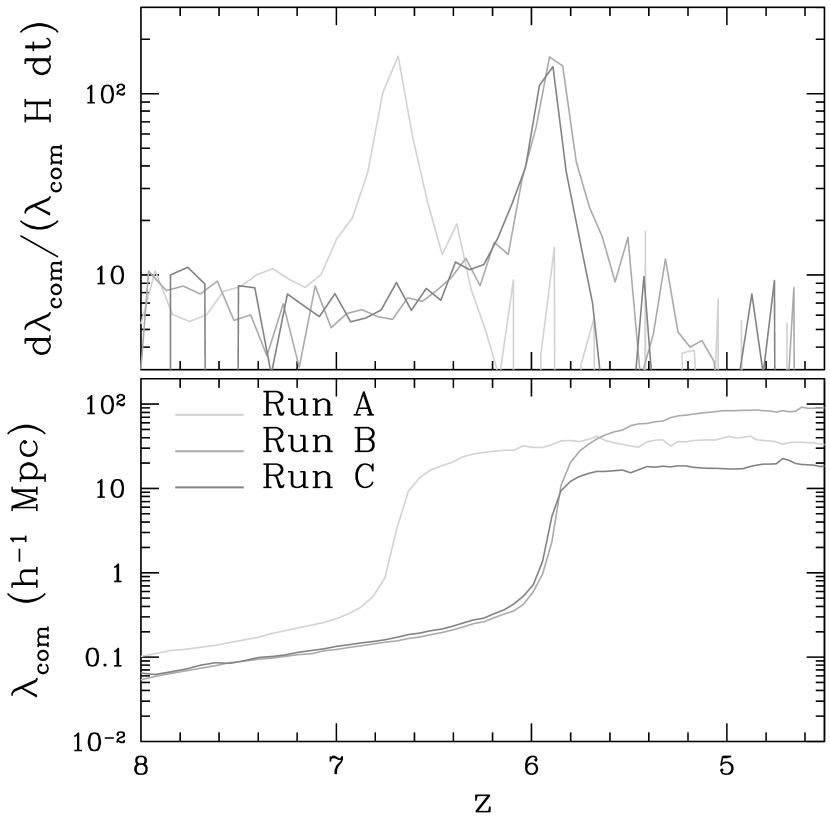
Figure 1: Mean free path to ionizing radiation (bottom) and its time derivative (top) as a function of redshift for the three simulations from Table 1.

Before one can attempt to measure “the redshift of reionization”, we better be sure that such a quantity can be defined. The whole process of reionization is quite extended ($\Delta z\sim 5-10$), and even the fast process of percolation of ionized bubbles occurs over a sizable redshift interval $\Delta z\sim 1$ [Gnedin 2000a]. However, one can still define the specific value of the redshift of reionization as the moment which corresponds to the peak rate of increase of the mean free path to ionizing radiation. As can be seen from Figure 1, the time derivative of the mean free path has a well defined peak, which I use throughout this paper as “the redshift of reionization” $z_{\rm REI}$.

4 Results

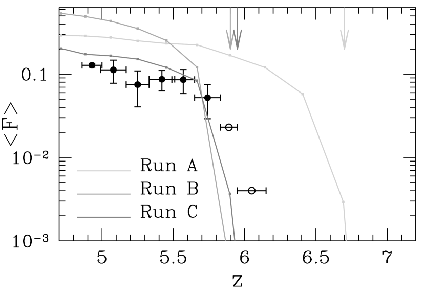
Figure 2: Mean transmitted flux as a function of redshift for simulations A-C. Points show the observational data from Becker et al. [Becker et al. 2001]. The last two data points (open circles) are obtained from only one quasar, and the vertical error due to cosmic variance cannot be estimated. Arrows mark the redshift of reionization for each simulation.

Figure 2 shows the mean transmitted flux as a function of redshift for the three simulations described above. In each case the arrow shows the redshift of reionization, and points with error-bars are taken from Becker et al. [Becker et al. 2001]. Each point represents an average of up to four quasars, except for the last two points that are derived from a single quasar and thus have no vertical error-bars. It is important to emphasize that the measurement of the mean transmitted flux for each quasar over an interval $\Delta z\approx 0.15$ is quite accurate, with the intrinsic error of only $0.003-0.005$ in $\langle F\rangle$, but the variation between different lines of sight (the so-called “cosmic variance”) is much greater, and it is this variation that dominates the vertical error-bar. Thus, one (or better two) more $z=6.3$ quasars are required in order to place the vertical error-bars on the open circles. However, because the sharp drop in the mean transmitted flux at $z\approx 6$ is marked by two data points, it is more reliable than simply one point from one quasar.

Simulations in Fig. 2 differ from the data points in two ways: both the redshift evolution in a simulation and the photoionization rate after reionization (the amplitude of the curve at low $z$) are offset relative to the data. As I mentioned above, the free parameter $\epsilon_{\rm UV}$ can be used to adjust the simulation to fit the observational data. However, there is no guarantee that with one parameter I can adjust two offsets at the same time for a given cosmological model. This fact is extremely important because it allows one to actually put constraints on the cosmological model per se, and I elaborate on this opportunity in the conclusions, but here I am going to ignore this fact and adjust two offsets independently - by sliding the curve both vertically and horizontally - to fit the observational data. Because the three curves from three simulations have similar shapes, every simulation can thus be made to fit the data - and, again, in reality, only a narrow range of cosmological models will succeed in doing so.

The reason for doing so is to obtain a constraint on the redshift of reionization which does not depend on a (weakly constrained) cosmological model. In addition, the simulations presented here are rather small and numerical errors due to incomplete convergence are substantial [Gnedin 2000a]. Simulations with larger box sizes typically have lower mean transmitted flux after reionization than small box simulation - which implies that amplitudes of three curves are not sufficiently accurate in Fig. 2. The arbitrary vertical shift of the curves can thus be considered as a “marginalization” over the simulation box size.

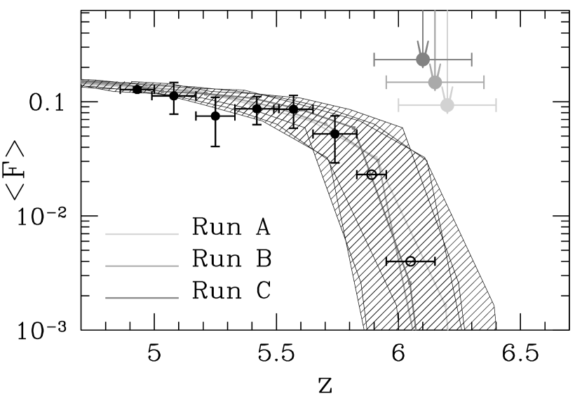
Figure 3: Mean transmitted flux as a function of redshift for simulations A-C, fitted to the observational data from Becker et al. [Becker et al. 2001] by shifting curves both in vertical and in horizontal direction. Shaded regions illustrate the uncertainty due to observational errors; this uncertainty is also given by the error-bars drawn on the arrowheads.

Figure 3 shows the fit to the observational data for each of the three simulations. The shaded region also gives an uncertainty of this fit, which can be considered a random uncertainty due to observational errors (mostly cosmic variance). Because the last two points have no vertical error-bars, they are only partly used: they only constrain models in the horizontal direction, and their redshift error-bars uncertainty are somewhat arbitrarily increased by a factor of 2 (to account for the possibility that they can be moved up and down). The fact that different cosmological models have slightly different redshifts of reionization when made to fit the observed evolution of the mean transmitted flux illustrates the systematic uncertainty due to unknown cosmological parameters. With these two uncertainties included, I can derive a value for the redshift of reionization in the following form:

$$z_{\rm REI}=6.2\pm 0.1{\rm s}\pm 0.2{\rm r},$$ (1)

which is the sole result of this paper.

If cosmic variance on the last two points can be estimated, and if it is comparable to the vertical error-bar on the $z=5.7$ point, then the random error gets reduced from 0.2 to 0.1.

5 Conclusions

SLOAN observations of $z\sim 6$ quasars push the frontier of the observable universe right into the epoch of reionization. Combined with the most advanced simulations of cosmological reionization to date, the observational data yield a rather precise measurement of the redshift of reionization.

This measurement hinges on the assumption that the $z=6.28$ quasar (SDSSp 1030+0524) probes an average region of the universe, i.e. that the cosmic variance in the measurement of the mean transmitted flux at $z=6.1$ is not larger than a factor of 3-5. One or two more $z=6.3$ quasars are required to confirm or refute this assumption.

A strong sensitivity of the redshift of reionization to the amount of small-scale power offers a unique opportunity to place constraints on the slope of the primordial power spectrum - unattainable even with the SLOAN data on the power spectrum at megaparsec scales. For example, runs B and C in Fig. 2 have similar star formation rates and redshifts of reionization, but differ by a factor of 3 in the mean transmitted flux at $z=5-5.5$ only because the slope of the primordial power spectrum $n$ differs by mere 0.02 in the two models. Sufficiently large simulations that have numerical effects under control are currently feasible and will eventually provide a tight constraint on the amount of small-scale power.

References

- [Becker et al. 2001] Becker, R. H., et al. 2000, AJ, in press (astro-ph/0108097)
- [Djorgovski et al. 2001] Djorgovski, S. G., Castro, S. M., Stern, D., Mahabal, A. 2001, ApJL, in press (astro-ph/0108069)
- [Gnedin 2000a] Gnedin, N. Y. 2000a, ApJ, 535, 530
- [Gnedin 2000b] Gnedin, N. Y. 2000b, ApJ, 535, L75
- [Gnedin & Abel 2001] Gnedin, N. Y., Abel, T. 2001, NewA, in press (astro-ph/0106278)
- [Miralda-Escudé 1998] Miralda-Escudé, J. 1998, ApJ, 501, 15
- [Steidel et al. 1999] Steidel, C. C., Adelberger, K. L., Ciavalisco, M., Dickinson, M., Pettini, M. 1999, ApJ, 519, 1