Detection and Measurement from Narrowband Tunable Filter Scans

Abstract

The past five years have seen a rapid rise in the use of tunable filters in many diverse fields of astronomy, through Taurus Tunable Filter (TTF) instruments at the Anglo-Australian and William Herschel Telescopes. Over this time we have continually refined aspects of operation and developed a collection of special techniques to handle the data produced by these novel imaging instruments. In this paper, we review calibration procedures and summarize the theoretical basis for Fabry-Perot photometry that is central to effective tunable imaging. Specific mention is made of object detection and classification from deep narrowband surveys containing several hundred objects per field. We also discuss methods for recognizing and dealing with artefacts (scattered light, atmospheric effects, etc.) which can seriously compromise the photometric integrity of the data if left untreated. Attention is paid to the different families of ghost reflections encountered, and strategies to minimise their presence. In our closing remarks, future directions for tunable imaging are outlined and contrasted with the Fabry-Perot technology employed in the current generation of tunable imagers.

1 Introduction

Imaging Fabry-Perot interferometers are now in common use at several major observatories and operate at both optical and infrared wavelengths. Traditionally, Fabry-Perots are employed to perform studies of extended gaseous nebulae. Examples include outflow sources (starburst and active galaxies, Herbig-Haro systems) and normal disk galaxies. Some groups have utilised the angular spectral coverage to detect diffuse sources (HI/Ly$\alpha$ clouds in optical emission), by azimuthally summing deep Fabry-Perot images (Haffner, Reynolds & Tufte 1999). More recently, scanning Fabry-Perots have been used to construct spectral line profiles at many pixel positions across a large format CCD. In many instances, these spectra are used simply to obtain kinematic information (line widths, radial velocities) in a strong emission line (e.g. Laval et al.  1987; Cecil 1988; Veilleux, Bland-Hawthorn & Cecil 1997; Shopbell & Bland-Hawthorn 1998). At lower spectral resolutions, tunable filters are a special class of Fabry-Perot, with which a series of narrowband images, stepped in wavelength, can be obtained (Atherton & Reay 1981; Bland-Hawthorn & Jones 1998a,b; Jones & Bland-Hawthorn 2001). Alternative modes see the Fabry-Perot used for time-series imaging (Deutsch, Margon & Bland-Hawthorn 1998; Tinney & Tolley 1999), which we do not discuss here. It is less common to see these instruments employed as spectrophotometers where the observed signal is calibrated to exoatmospheric flux units. This may be due, in part, to a perception that the nature of the Airy function makes Fabry-Perots unreliable photometers.

In this review, we describe reliable methods for flux-calibrating Fabry-Perot data with the aid of worked examples. The case of tunable imaging is special, in that photometric measurements centre upon the measurement of low resolution spectra and extraction of objects with candidate emission or absorption features. In this sense it is analogous to multi-slit or multi-fibre spectroscopy. However, because the tunable filter images all objects in the field at once, every object is a potential candidate. Therefore, data reduction and methods need to be devised so as to be fully automated throughout. In deep extragalactic surveys at high galactic latitude, the number of objects can vary anywhere between a few hundred in high galactic latitude fields to over a thousand in galaxy clusters.

This paper reviews all stages of analysis, discussing different approaches where they exist. Section 2 describes features of tunable filter use and Section 3 defines terminology used throughout the rest of the paper. Section 4 discusses different methods for the removal of instrumental signatures while Section 5 reviews strategies for the detection and classification of the many objects in a single field. Flux calibration issues are discussed in Section 6 and concluding remarks follow. Many of the procedures described here have been written into software (Jones 1999). Interested prospective users are encouraged to contact the authors and visit the Taurus Tunable Filter (TTF) web page.

2 The Nature of the Observations

At optical and infrared wavelengths, imaging Fabry-Perot devices are used in three different ways: (i) to obtain a spectrum at each pixel position over a wide field by tuning the etalon, (ii) to obtain a single spectrum of a diffuse source which fills a large fraction of the aperture (from one or more deep frames at the same etalon spacing), and (iii) to obtain a sequence of monochromatic images within a field defined by the Jacquinot spot (tunable narrowband imaging). Figure 2 summarises the different modes and the types of data they produce. In this paper, we will concentrate on analysis techniques adapted for final case, tunable filter imaging. However, many of the methods presented herein are common to all three modes of operation.

Observations of a particular field consist of one of more sets of images called a scan (or a stack or spectral cube). A scan is a series of images (or slices) in which each one has been taken at a slightly different plate spacing. This is achieved by tuning the filter to a new passband between each exposure. Ideally, scans should be repeated three or more times to permit median-filtering of cosmic-ray events and ghost images from slices of common wavelength. Removal of ghosts requires the telescope to be offset between scans and the Fabry-Perot to be tilted to ensure separation of ghosts and parent sources. In this situation, the ghosts will shift in the opposite direction to the parent objects and by twice the amount.

At a given (constant) order of interference, a one-to-one relationship exists between plate spacing and image wavelength. At the telescope, the spacing is encoded in software units known as Z-step values, due to the movement of the Fabry-Perot plates during both tuning and scanning. Wavelength calibration frames take the form of long “sausage-cubes”: small images (few pixels square) at many wavelength settings (typically 100 or more). The small image area permits expediency while scanning the plates at sufficiently high sampling resolution.

If the Fabry-Perot is used in the pupil (as is usually the case), a phase effect shows itself as a position-dependent change in wavelength across the field. Figure 4($a$) illustrates this with data from the Taurus Tunable Filter (TTF) system (Bland-Hawthorn & Jones 1998a,b) at the Anglo-Australian Telescope (AAT). The centre of the interference pattern is coincident with the optical axis and the distance of an object from this point is its optical radius. The phase change over the field gives rise to night-sky rings, broad diffuse circles of atmospheric OH emission lines on some images, centred on the optical axis (Fig. 4$b$). They are circular because the phase change makes for a specific off-axis angle where the interference equation is satisfied for a specific wavelength. For cases in which this effect is present, the flux needs to be re-normalised in radial bins, since it is not corrected through division by a flatfield. If a tunable filter is used in the field (i.e. after the field lens) then the abovementioned effect does not occur. Meaburn (1976) shows examples of this arrangement for Fabry-Perot devices used in the near infrared.

The underlying principle of a tunable filter is the enlargement of the Jacquinot spot at narrow plate spacings, and therefore, low spectral resolutions. The Jacquinot spot is defined as the field about the optical axis within which the peak wavelength variation with field angle does not exceed $\sqrt{2}$ of the etalon band-pass (Jacquinot 1954; Taylor & Atherton 1980). This angular field can be used to perform close to monochromatic imaging.

3 Definitions

3.1 The Instrumental Response Function

The most direct route to the Airy function, the instrumental response of the Fabry-Perot, is to use complex exponential notation. An incoming plane wave with wavelength $\lambda$ at an angle $\theta$ to the optical axis enters the etalon cavity and performs a series of internal reflections. If the highly reflective inner surfaces have reflectivities of ${\cal R}_{1}$ and ${\cal R}_{2}$, we can sum over the complex amplitudes of the outgoing plane waves such that

$${\cal I}=1+{\cal R}_{1}{\cal R}_{2}e^{2i\delta}+{\cal R}_{1}^{2}{\cal R}_{2}^{2}e^{4i\delta}+....={{1}\over{1-{\cal R}_{1},{\cal R}_{2}e^{2i\delta}}}$$ (1)

in which $2\delta$ is the phase difference between successive rays. The total transmitted intensity is proportional to the squared modulus of the complex amplitude or

$${\cal A}={\cal I}{\cal I}^{*}={{1}\over{1+{{4{\cal N}^{2}}\over{{\pi}^{2}}}sin^{2}2\pi\mu l\lambda^{-1}\cos\theta}},$$ (2)

where the refractive index and the plate separation of the cavity are $\mu$ and $l$ respectively, and ${\cal N}=\pi\sqrt[4]{{\cal R}_{1}{\cal R}_{2}}(1-\sqrt{{\cal R}_{1}{\cal R}_{2}})^{-1}$.

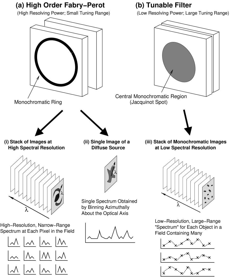
Figure 2: Different modes of Fabry-Perot use in the case of both ($a$) high resolution instruments, and ($b$) tunable filters.

Clearly, the Airy function has a series of periodic maxima whenever

$$m\lambda=2\mu l\cos\theta$$ (3)

which is the well-known equation of constructive interference in the $m$th order, with $\theta$ being the off-axis angle of the ray, (as subtended at the etalon), and $\mu=1$, since the Fabry-Perot is air-spaced. The quantity ${\cal N}$ is called the reflective finesse and depends only on the values of ${\cal R}_{1}$ and ${\cal R}_{2}$. It is normal procedure to manufacture an etalon with two identical coatings such that ${\cal R}_{1}={\cal R}_{2}$, but in App. B we describe the extraneous etalon effect, where this condition is not met.

Figure 4: ($a$) Contour plot showing the change in wavelength across the field. In this example, the values at the top of the panel are order of interference (left) and effective plate spacing (right). ($b$) Raw image showing the ring pattern of atmospheric night-sky emission lines resulting from a wavelength gradient across the field. The wavelength contours in ($a$) match those of the image in ($b$).

Figure 6: Three cyclic functions listed in Table 1 (column 2) shown at low finesse to emphasize their differences.

Figure 8: The integral of the Airy curve as a function of finesse normalized with respect to the Gaussian and Lorentzian integrals. The asymptotic limit of the upper curve is $\sqrt{\pi\ln 2}$.

In order to arrive at the correct calibration procedure, it is important to understand the nature of the Airy function. Figure 6 illustrates the three cyclic functions in Table 1 and shows that the area of the Airy function always exceeds the integral of the other functions for a given spectroscopic resolution. By analogy with the Lorentzian profile, the coefficient of the $\sin^{2}$ factor in Eqn. (2) determines the width of the function. The quantity $\Delta x/\delta x$ is called the effective finesse, where $\delta x$ is the spectral purity (defined in Eqn. (7) below) and $\Delta x$ is the periodic free spectral range. In Fig. 8 we illustrate how the Airy function, when normalized to the Gaussian and Lorentzian functions, depends on ${\cal N}$. In practice, there are factors other than coating reflectivities which contribute to the effective finesse $-$ aperture effects, imperfections within the plate coatings, etc. $-$ some of which can serve to make the instrumental response more Gaussian than Lorentzian in form (Atherton et al.  1981).

Beyond a finesse of roughly 40, the Airy function is highly Lorentzian. The reason for this is clear when looking at how the Airy profile has been written in Table 2. At high finesse ($\Delta x>>\delta x$), if we expand $x$ about the peak of the profile, the small angle formula reduces the Airy function to the Lorentzian form. The normalized Airy integral depends only weakly on finesse at large finesse values.

3.2 The Jacquinot advantage

There are several approaches to deriving the Jacquinot advantage (Roesler 1974; Thorne 1988), i.e. the throughput advantage of the Fabry-Perot interferometer. By considering the solid angle subtended by the innermost ring and using the small angle formula with Eqn. (3), we arrive at the important relation

$$\theta^{2}={2\over R}={\Omega\over\pi},$$ (4)

which assumes that $\mu=1$ and that $\Omega$ and $R$ are the solid angle and spectral resolving power of the ring, respectively.

This equation has been used to demonstrate that Fabry-Perot interferometers, at a given spectroscopic resolution, have a much higher throughput than more conventional techniques (Jacquinot 1954; 1960). But the Jacquinot relation has another important consequence. The solid angle of a ring defined by its FWHM intensity points can also be written

$$\Omega=2\pi\theta\ \delta\theta=\pi\lambda({\cal N}l)^{-1}.$$ (5)

For a fixed etalon spacing, the solid angle, and hence the spectroscopic resolution, of all rings is a constant. This allows us to write down a simple equation valid for all rings for the signal-to-noise ratio in a monochromatic unresolved line, namely,

$${\rm SNR}=s\sqrt{\frac{(\epsilon\tau\eta)\left({\delta\lambda^{\prime}}\over{\delta\lambda}\right)\left({\Omega\over\omega}\right)}{(s+b+\frac{f\ \delta\lambda}{\delta\lambda^{\prime}\epsilon\tau}\sigma^{2}_{R})}}$$ (6)

where $s$ and $b$ are the source and background flux (cts pix^-1 s^-1), $\epsilon$ and $\tau$ are the efficiency and exposure times respectively, $\omega$ is the solid angle subtended by a pixel. The quantity $\delta\lambda^{\prime}$ is the wavelength dispersion (Å pix^-1) and $f$ is the number of CCD exposures combined to form the deep spectrum. The factor $\eta$ is discussed below. We normally choose to place the ring center at one corner of the field for two reasons. First, it is often necessary to tilt the etalon in order to throw ghost light out of the field. Second, the factor $(\Omega/\omega)^{0.5}$ in Eqn. (6) now ensures that the spectroscopic sensitivity is constant over most of the field. There will be an almost linear drop-off in sensitivity at large off-axis angles (far corner from the optical axis) where the rings become seriously incomplete.

An important characteristic of a spectrometer is its spectral purity,

$$\delta x=\frac{\int_{0}^{du}{\cal A}(u)\;du}{\int_{0}^{\pi}{\cal A}(u)\;du}=\frac{2}{\pi}\tan^{-1}\Bigl{(}\frac{2{\cal N}}{\pi}\tan\frac{\pi}{{\cal N}}\Bigr{)},$$ (7)

namely, the smallest measurable wavelength difference at a given wavelength (Thorne 1988). This is usually defined as the intensity FWHM of the instrumental profile. When considering the amount of light transmitted by a spectrometer, we need to consider the total area under the instrumental function. This issue is rarely mentioned in the context of long-slit spectrometers partly because their response is highly Gaussian, in which case the ‘effective photometric bandpass’ (total area divided by peak height) is very close to the FWHM of the instrumental profile (see Table 2).

High spectral purity does not necessarily equate with high efficiency. At values of low finesse, the efficiency is high but spectral purity is compromised by the amount of power in the wings, thereby reducing spectral definition (Fig. 10). Conversely, at high finesse a sharper instrumental profile is marred by a loss in efficiency. The optimal trade-off lies with values of finesse in the range ${\cal N}=30$ to 40.

Figure 10: A plot of efficiency against effective finesse for $R$ and $K$-band Queensgate etalons. The $R$-band calculation is for a wavelength of 6700Å and a plate flatness of $\lambda/150$ (after coating), measured at 6330Å. The $K$-band etalon is for a wavelength of 2.2$\mu$m and a plate flatness of $\lambda/50$. The curves decline less rapidly if a higher plate flatness is achieved. We have included losses of 0.2% due to coating absorption and scattering; these tend to have more effect at higher finesse. The dashed curve shows how the finesse depends on the coating reflectivity.

At such moderate finesse, the Airy function allows through 50% more light than a Gaussian profile with equal spectroscopic resolution (Fig. 8). Thus, the effective photometric bandpass, $\delta\lambda_{\rm e}$, is almost 60% larger than the bandpass defined by the profile FWHM $\delta\lambda$. The factor $\eta$ in Eqn. (6) corrects for a calculation based on the FWHM of a ring and is defined as $\delta\lambda_{\rm e}/\delta\lambda$. Technically, $\delta\lambda_{\rm e}$ should be adopted as the spectral resolution of the Airy instrumental profile, otherwise we are forced to an inconsistency when comparing Fabry-Perot spectrometers to other devices.

Using the Fabry-Perot as a tunable filter necessitates tuning the bandpass to several discrete wavelengths and obtaining an image at each. Figure 12 shows such an arrangement for the TTF Field Galaxy Survey, made with TTF at the AAT (Jones 1999). Also shown in this figure are the filters used to block light transmitted at unwanted neighbouring orders. The ideal spacing of bandpasses for such detection/photometry applications is $\pi/4\times{\rm FWHM}$, which is half of the effective photometric bandpass. However, for kinematic work, this sampling should be increased to ${\rm FWHM}/2$.

Figure 12: Passband sampling used in the TTF Field Galaxy Survey scans through ($a$) 707/26, ($b$) 814/33 and ($c$) 909/40 nm blocking filters. The extent of each blocking filter is also shown (dotted lines). Note that the wavelength scale differs between panels.

4 Data Reduction

4.1 Flatfield Correction

It is hard to overstate the importance of the whitelight cube. This is obtained by observing a whitelight source over the same range of etalon spacings used in the actual observations. The whitelight cube maps the response of the filter as a function of position and etalon spacing. There are three effects that we wish to divide out from the data. Firstly, the narrowband filter response, when convolved with the instrumental response, leads to a modulation in the observed spectrum. Secondly, it is well known that filters have variable responses in both collimated and converging beams (Lissberger & Wilcock 1959). Thirdly, we seek to remove any inhomogeneities in the filter structure as a function of position. When the whitelight cube is compressed in the spectral dimension, it provides a very high signal-to-noise flatfield for removing pixel-to-pixel sensitivity variations.

Several approaches exist for the creation and use of whitelight flatfields, depending on the exact nature of the data. Dome flats do not mimic the sky well in cases where light scatters off the dome and irradiates the detector at extreme angles. This can fill in the whitelight response structure with wavelength. Alternatively, twilight flatfields contain Fraunhofer lines which generate fringe structure not present in science data. The underlying point is that both the spatial and spectral distribution of the flatfield source must be well-understood for its proper use in removing pixel variations.

Final flatfields can be constructed from raw flatfield frames in one of two ways, dependent upon whether interference fringes are present in the CCD used. Such fringes are due to interference within the substrate of the CCD at red wavelengths and are unrelated to the interference within the Fabry-Perot. In the absence of fringing the flatfield frames can be normalised and retained as individual components of the scan, and used to divide images on an individual basis in the usual way. If fringing is present in both the flatfields and science frames, division of the latter by the former can be tried, but its success relies on the stabilty of the fringe pattern. Typically, Fabry-Perot plate spacings are not sufficiently stable to produce fringe structures constant over the hours that pass between flatfields and science frames. Alternatively, a fringe correction frame can be created by combining the science frames at a given etalon setting, using median filtering to remove the objects in the field, (assuming that the object position has been dithered between exposures). This produces a final frame of the fringe pattern alone, which can be subtracted. However, the same technique can not be used for removing fringes from the flatfield. More elaborate operations can be adopted, usually at the expense of added noise to the frame cleaned of fringing. In the end one has to determine whether it is better to use a noisier frame cleaned of fringes, or a less noisy frame on which the fringes remain. This depends on the specific science requirements of the data.

While flatfields (used in either manner) successfully remove pixel-to-pixel variations, the instrumental response across the beam is modulated by the phase effect. In particular, care must be exercised in the use of flatfields near the edges of the blocking-filter transmission profile, as the effectiveness of the flatfield then becomes a function of optical radius. In the case of photometry of point-source objects, we can account for any residual radial changes in sensitivity by photometrically registering objects through a fit with optical radius at a later stage (Sect. 5.4).

4.2 Night-Sky Ring Removal

For detection of faint point-sources, night-sky rings need to be removed so that the detection software can successfully fit the sky background, (which is typically done through the use of a two-dimensional sky mesh.) Although the rings look circular, they are in fact slightly elliptical (0.5%) due to the imperfect alignment of the CCD plane and optical distortions within the focal reducer.

Glazebrook & Bland-Hawthorn (2001) have demonstrated that the night sky lines can be removed from data to the level of 0.03% or better using nod and shuffle techniques. Here, the telescope is nodded between the object and sky positions in synchrony with charge being shuffled on the CCD with a cycle time of, say, 60 secs. This results in a 50% loss of observing efficiency but does in fact lead to superb sky subtraction. Nod and shuffle with TTF produces almost perfect residuals largely because there is no entrance slit, and the monochromatic band is sampled by hundreds of CCD pixels along the optical radius vector.

In those cases where nod and shuffle is not available or not feasible, alternative ways of removing the sky can be followed. If the sky background and night sky lines can be taken as having a fixed pattern across the field of view – usually a safe assumption for the relatively small field and long exposure times of the TTF – the problem of sky subtraction can be most readily approached by exploiting the azimuthal symmetry of the sky component relative to the optical axis. A flat sky will be evident in the data as a radial variation in the background, with night sky lines appearing as broad rings. To parameterize the spectrum of the sky, the basic method is to azimuthally bin the image about the optical axis. Bright stars and regions of evident emission are masked from the image prior to the binning procedure. The sky spectrum is then calculated from the masked image using a median combination of the pixels remaining at each radius. The median will eliminate fainter emission that the mask may have missed and additional cosmic rays.

The position of the optical axis is crucial to determining the accurate phase error over the field. There are several ways to find its location:

1. If the tunable filter can be tuned to an interference order $m>70$ or so, the monochromatic ring will be narrow enough to be fit with least-squares techniques. Specific procedures for fitting the rings are discussed below and in App. A.

2. We can generate a well-defined ring by differencing two low order monochromatic scans where one is tuned slightly in $Z$-space (e.g. half a bandpass) compared to the other. The residual produces a P-Cygni profile along the optical radius passing through zero counts which can then be fit with standard procedures discussed below and in App. A. This residual image is typically very flat and not susceptible to CCD bias, flatfield or response variations.

3. Diametric ghosts can be very useful for identifying the optical axis since these, by definition, reflect about the optical axis. One technique is to generate the ghost map by imaging through a mask of pinholes arranged in a regular grid. At the AAT we use a matrix mask consisting of 100$\mu$m holes drilled every 1 cm. The optical axis can then be identified as the crossing point for all vectors which join the pinhole images with their respective ghosts (Fig. 14).

   

   Figure 14: Use of a pinhole mask image to find the optical axis. The ghost image of each pinhole is diametrically reflected about the optical centre. The intersection of two or more lines joining pinhole images to their corresponding ghost images will give the location of the optical axis.

4. A more involved approach is to derive the phase surface by scanning the TTF over a strong emission line (Bland & Tully 1989). Each spectrum within the monochromatic cube must now be fit with Lorentzian profiles. The resulting surface is highly paraboloidal and the optical axis along its centre is well defined.

A quick method for finding the approximate centre of the night-sky ring pattern is to solve the equation of a circle from three points. However, for the purpose of subtraction, circular fitting is usually insufficient and more sophisticated strategies must be adopted (App. A). Once the sky spectrum has been determined, a two-dimensional sky “image” can be constructed by sweeping the sky spectrum azimuthally around the position of the optical axis, in effect reversing the binning procedure. This sky image may then be subtracted from the data image. As is illustrated in Fig. 16, this procedure works quite well for sparse fields, where only a small percentage of the pixels need to be masked from the binning calculation. We note that this method works best if one gives some consideration to the placement of the optical axis at the time of observation: within the field of view but away from the object of interest. Placement should also ensure that bright ghosts in the field are avoided.

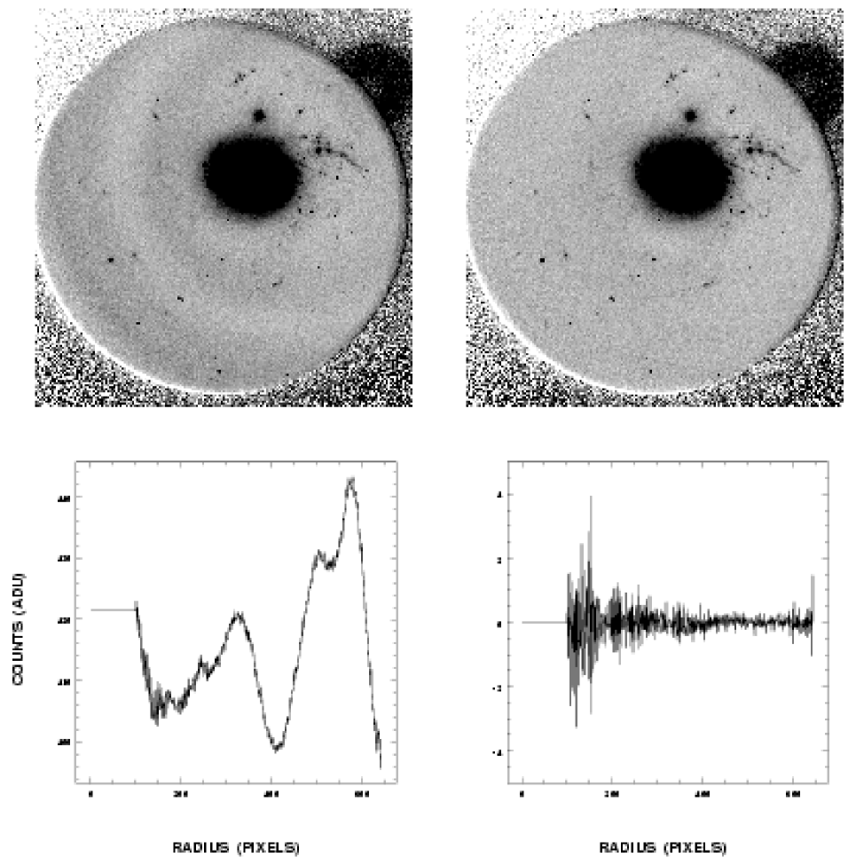
Figure 16: Example of night-sky ring removal using azimuthal fitting and subtraction. (Left) Sky ring pattern on the original image with a cross-section (below) showing the amplitude of the variation. (Right) The same image and cross-section following subtraction. Note that the remaining faint background structure in this case is real.

In those cases where the field is densely populated, the empirical removal of a uniform azimuthal sky component may not be feasible. At this point, the sky rings must be individually fit and parametrized. The core of the fitting problem is that the sky-rings are typically incomplete, passing beyond the field-of-view for part of their length. Defining the problem as minimising the sum of squares, the so-called geometric distance, is computationally very expensive and requires careful weighting schemes and application (e.g. Joseph 1994). After years of experimentation with conventional methods (e.g. Bland-Hawthorn, Shopbell & Cecil 1992), we have settled on algebraic distance methods as the most economical and reliable approach to fitting incomplete arcs, as described in App. A. One persistent problem has been the geometric distortion of Cassegrain focal reducers exacerbated by slight tilts in the alignment of the CCD plane.

An alternative method for removal is feasible in the case where the objects of interest are much smaller than the ring structure (e.g. at very low spectral resolution when the night-sky rings are large and diffuse). The rings are removed by treating each science exposure individually. A background map is created by median-filtering copies of the original, each one offset in a regular grid pattern from the other by a few pixels. The result is then smoothed and subtracted from the original, leaving little or no night-sky residual. The method depends upon the rings being of lower spatial frequency than the objects, and as such, would be less successful with extended sources. Bland-Hawthorn & Jones (1998b) demonstrate this technique with an example.

4.3 Wavelength Calibration

The tunable filter is wavelength-calibrated through scans consisting of many images taken at a series of gap spacings. Spacing through the scan is controlled in software through a parameter, $Z_{s}$, of arbitrary units and proportional to physical plate spacing. Ordinarily, two scans are required: an emission-line scan of an arc lamp such as copper-argon or neon, and a continuum scan of a white-light source such as a tungsten lamp (the white-light calibration cube), as mentioned earlier.

It is essential that both types of source are diffused by suitable optics. Past experience has shown that anomalous phase effects are produced by incorrect use of calibration lamps. They must illuminate the instrument evenly and should not be placed between the telescope focus and the CCD.

An additional consideration in the choice of a suitable arc lamp is that a minimum of two lines, (preferably more), should be visible within the restricted wavelength coverage of the blocking filter (typically 25 to 30 nm). Lamps in use with TTF system at the AAT are shown in Table 4. Around 500 nm, the astrophysical lines of H$\beta$ $\lambda$4861 and [O iii] $\lambda\lambda$4959,5007 found in planetary nebula are a suitable alternative, and Acker et al.  (1992) list many suitable objects.

The continuum scan (Fig. 18$a$) is used to check where (in $Z_{s}$) the orders of interference occur and to ensure no overlap. Continuum scans can be sampled quite coarsely ($\Delta Z_{s}>20$) and should cover a range of more than one order, since the location of these is not known at the outset. Overlap of the resulting blocking filter traces indicates a plate spacing that is too large, causing the sampling of more than one order of interference. Once two orders have been located, a well-sampled scan ($\Delta Z_{s}\sim 3$) through an arc lamp can follow (Fig. 18$b$). Such a scan covers more than one order so that at least one arc line appears in adjacent orders. This is necessary for a determination of physical plate spacing. Typically the number of arc lines available over the wavelength coverage of the blocking filter is few. The two profiles in Fig. 18($b$) show the wavelength offset between on and off-axis positions.

Lines observed in the emission-line scan are identified both by the wavelength and $Z_{s}$ at which they occur. Across a single order, the $(Z_{s},\lambda)$ relationship is linear,

$$\lambda(Z_{s})=C_{1}Z_{s}+C_{2}.$$ (8)

To determine the plate-spacing in physical units (such as microns) we need to first determine the order of interference. If $\Delta Z_{0}$ is the free spectral range (in $Z_{s}$-units) separating an arc line (wavelength $\lambda_{0}$) in adjacent orders, then the order of interference $m$ is given by

$$m=\frac{\lambda_{0}}{\Delta Z_{0}\cdot C_{1}}.$$ (9)

With $m$ known, the spectral resolving power $R$ and passband width $\delta\lambda$ can be determined through

$$N_{\rm R}\cdot m=\frac{\lambda_{m}}{\delta\lambda}=R.$$ (10)

The large scan range of TTF sees resolving powers anywhere in the range of 150 to 1000. The physical plate-spacing calibration follows as an adaptation of Eqn. (8), namely

$$L=\frac{m}{2\cos\theta_{\rm off}}\cdot\Bigl{(}C_{1}Z_{s}+C_{2}\Bigr{)},$$ (11)

where $L$ is the effective plate spacing and $\mu=1.00$ for air. By effective plate-spacing, we mean the gap as measured parallel to the optical axis, irrespective of etalon tilt. The true gap between the plates is smaller than this, being $L\cos\alpha$, where $\alpha$ is the tilt of the etalon, (typically a few degrees to deflect ghosts out of the beam).

At very narrow gaps ($\lower 2.15277pt\hbox{$\;\buildrel<\over{\sim}\;$}3$$\mu$m), there is a wavelength-dependent phase-change in the reflections between optical coatings on the inner plate surfaces. This introduces a degeneracy that requires an additional term to be introduced into Eqn. (3). The effect can be measured at such narrow plate-spacings, provided the phase-change behaviour of the inner coatings has been determined through independent means (Jones & Bland-Hawthorn 1998).

The angle $\theta_{\rm off}$ in Eqn. (11) is that separating the rays on-axis and those sampled for calibration. The wavelength offset between both points must be included in the calibration, through relations derived in Bland-Hawthorn & Jones (1998a,b). For example, suppose that the point used on the detector is offset by 500 pixels from the optical axis. If the focal length of the camera is 130 mm and detector is a $1024\times 1024$ pixel CCD of $25\times 25$ mm, then

$$\theta_{\rm off}=\frac{500}{1024}\times\frac{25}{130}=0.094\,\,\,{\rm radian}.$$ (12)

If the observing conditions cause measurable drifts in wavelength of the etalon bandpass one can treat the affected frames as wavelength-averaged over the exposure time and bandpass from the time dependence. Temporal variations can be measured through rapid scans (either small pixel-area or charge-shuffle) and fit by a smoothly-varying function.

Figure 18: Example tunable filter calibration scans through the same blocking filter, showing ($a$) continuum, and ($b$) emission-line spectra. The two scans in ($b$) were measured on-axis (solid line) and off-axis (dotted).

4.4 Image Alignment

The offsets introduced for ghost-image removal necessitate spatial registering of scans. There is distortion present in the field extremities of many focal reducers used to accommodate Fabry-Perot instruments, including the Taurus-2 focal reducer on the AAT. To measure this, we use a matrix mask consisting of 100$\mu$m holes drilled every 1 cm. Figure 20 shows a measurement of this by C. G. Tinney through the residual of the distorted radial distance ($\rho$, as measured at the detector) against that undistorted ($r$). At the largest radii the maximum distortion is 2%, and relative astrometry to better than 0.1 pix (0.03^′′ at f/8) is possible. The radial correction function requires terms up to $\rho^{4}$. Scan images need not be corrected for this provided the dithering is small ($\lower 2.15277pt\hbox{$\;\buildrel<\over{\sim}\;$}10$^′′). Bacon, Refregier & Ellis (2000) give an elegant treatment of the general solution to image distortions across a field (their Sect. 5), which can also be applied to tunable filter data in which high spatial precision is required.

Figure 20: Radial distortion in the Taurus-2 focal reducer of the AAT, as measured across the focal plane by C. Tinney using an MIT-LL CCD (15$\mu$m pixels). The residuals between the distorted ($\rho$) and undistorted ($r$) radii have been plotted and fit with the power law shown at top.

4.5 Variations in Seeing

Typically it takes several hours to complete scans and as such, the observations are susceptible to changes in seeing between individual frames. In such cases it is necessary to create a second version of the scan, in which all images have been degraded to the mean seeing $\langle W_{\rm w}\rangle$ of the worst frame in the original scan. This is done by covolving each original frame with a gaussian kernal of FWHM

$$\langle W_{\rm k}\rangle=\sqrt{{\langle W_{\rm w}\rangle}^{2}-{\langle W_{0}\rangle}^{2}},$$ (13)

where $\langle W_{0}\rangle$ is the mean seeing FWHM of the given frame. Both the convolved and unconvolved (original) versions of the scans are used for the subsequent analysis.

4.6 Co-addition of Image Stacks

For the best detection and photometry of a field, there should be three or more scans (as separate measurements), with slices $S(k,\lambda_{1})$, $S(k,\lambda_{2})$, …, $S(k,\lambda_{n})$, where $n$ is the number of slices per scan and $k$ is the scan number (up to the maximum $K$ scans taken). Each image corresponds to its central wavelength $\lambda_{i}$, ($1\leq i\leq n$). There should also be matching frames $G(k,\lambda_{1})$, …, $G(k,\lambda_{n})$, that have been smoothed to match the worst seeing image. A final co-added narrowband scan can be obtained by combining each set of narrowband frames of common wavelength. With two versions of all frames (unconvolved and convolved), and two methods of combination (straight summation or median-filtering), three versions of the co-added scan are derived:

1. Straight summation of the convolved frames at each wavelength,

   $$\sum_{k=1}^{K}G(k,\lambda_{i}),~{}~{}~{}~{}~{}~{}~{}~{}~{}\forall\;i=1,\,\ldots,\,n,$$ (14)

2. Straight summation of the unconvolved frames at each wavelength,

   $$\sum_{k=1}^{K}S(k,\lambda_{i}),~{}~{}~{}~{}~{}~{}~{}~{}~{}\forall\;i=1,\,\ldots,\,n,$$ (15)

3. Median-filtering of the unconvolved frames at each wavelength.

Median-filtering cleans the cosmic-rays and ghost images from scan (iii). However, it also lowers the signal-to-noise ratio by 30% or more on the faintest objects, thereby making scans (i) and (ii) more sensitive. Scans (ii) and (iii) have the better spatial resolution but are inferior to scan (i) for seeing stability, and therefore, photometric integrity. Optimally, scans (ii) and (i) can be used for the object detection and photometry, while (ii) and (iii) are used to build cosmic-ray and ghost image catalogues.

5 OBJECT DETECTION AND CLASSIFICATION

5.1 Initial Object Detection and Photometry

Object detection and photometry on a stack of narrowband frames can be performed using any of the common software packages for detection and photometry of objects, such as SExtractor (Bertin & Arnouts 1996) or FOCAS (Valdes 1993). The prescriptions that follow were developed using SExtractor. However, FOCAS has also been used with similar tunable filter data (e.g. Baker et al.  2001).

The SExtractor algorithm initially sees images background subtracted and filtered with a convolution mask to optimise detection sensitivity. Candidate objects are found as connected pixels above the prescribed threshold and passed through a deblending filter to separate into nearby overlapping objects if this is the case. SExtractor accepts input in the form of one (or two) FITS images and several files. We can make use of the dual-image capability to detect objects on the straight-summed/unconvolved frames and then photometer these positions on matching straight-summed/convolved frames. Basic shape and positional properties are measured from the detection image while photometric parameters are obtained from the second.

In the analysis of a full scan, the detection threshold should be set sufficiently low that all objects are recovered throughout the stack, including some noise peaks. This ensures the faintest detections are not lost due to variations in background through the scan. The object-finding software can be run on each scan frame in turn, the catalogues of which can be concatenated into a full raw catalogue. Each entry of this is a single detection (or observation) in $(x,y,N)$-space, where $N$ is the image containing the detection at spatial coordinate ($x,y$).

As with all imaging surveys, an inherent problem is not knowing the size of each object before its detection. It is possible to use a series of apertures of increasing size to cover the range of expected object sizes. If the innermost aperture is set to 1.35 times the seeing, the signal-to-noise ratio is maximised for a spatially unresolved source (gaussian profile) in a background-limited noise regime. For the purpose of maximising signal-to-noise ratio, it is preferable for a non-optimal aperture to be too big rather than small.

5.2 Extraction of Object Spectra

It is necessary to group multiple wavelength observations of the same object together. A straightforward algorithm for processing the raw catalogue is as follows. The first observation is written to the object buffer, an array to store all observables for a given object from each slice. The remaining lines of the raw catalogue are then searched for $(x,y)$-matches to the object in the buffer. If all observations for the object are found, or the limiting search depth is reached, the contents of the object buffer are summarised and written to file. The next observation is written to the cleared object buffer and the process repeats. Depending on the nature of the fields observed, the raw catalogue can contain $\sim 10^{4}$ observations for a 10 slice scan. Each time the object buffer is complete, the contents should be checked for at least two observations before being considered as an “object”. Such a double-detection criterion provides a robust way of removing noise-peak and isolated cosmic-ray detections in an automated fashion. However, it also selects against emission-line detections in a single-frame. Given the difficulty inherent in distinguishing such detections from cosmic-rays and noise peaks without manual inspection, single-frame detections are more easily extracted separately.

Each double-detection object can be assigned an ID number and the distance of the object from the optical axis calculated and used to correct calibrated wavelengths for phase shift (Bland-Hawthorn & Jones 1998b). The signal-to-noise ratio can be determined for the full rage of aperture sizes and those from the optimal aperture retained. Below-threshold detections can be discarded. If the final catalogue contains mainly galaxies, then subset catalogues for bright stars should also be created. These are needed for photometric registering during emission-line candidate extraction (Sect. 5.4).

5.3 Cosmic Ray and Ghost Image Removal

At this stage in the reduction, most of the cosmic-rays present on the images should have been caught by the detection software. The minimum two-detection criterion also filters out those that the software misses. However, two classes of spurious object are missed by both methods. Firstly, a cosmic-ray that occurs close enough to a real object will avoid removal if not detected by the software as a separate entity. Left uncaught, it will appear as a flux change in the nearby object, with very similar characteristics as genuine emission-line flux on continuum. Secondly, ghost images are usually admitted by detection algorithms as real objects because they show little change in flux or position between the frames of a single raw scan. It is only through a frame-by-frame comparison with the cleaned images that they become apparent. Appendix B discusses the different types of ghost images and strategies for minimising their occurrence at the outset, before they become part of the data.

Such spurious detections can be handled through the compilation of a catalogue of all cosmic-ray and ghost-affected pixels in $(x,y,N)$-space, and cross-checked with the $(x,y,N)$ object list. Any matches in the latter can then be removed. The straight-summed and median-filtered scans (scans (ii) and (iii) of Sect. 4.6) can be searched by taking each matching pair of images and computing the ratio image

$$C(x,y)=\frac{S(x,y)+f_{1}}{f_{2}\times M(x,y)+f_{1}}.$$ (16)

Here, $S(x,y)$ and $M(x,y)$ are a pair of straight-summed and median-filtered images, $f_{1}$ is an offset that governs search sensitivity and $f_{2}$ is the ratio of the two images measured from stellar fluxes. Spurious pixels are those for which $C(x,y)$ exceeds $C_{\rm thresh}$, the cosmic-ray threshold, which is sensitive to $f_{1}$. The parameter $f_{1}$ should be fixed 100 and 500 ADU) while $f_{2}$ and $C_{\rm thresh}$ vary freely with each image $N$. Trial divisions can be used to optimise these parameters. The final cosmic-ray/ghost catalogue is used in the emission-line search described in Sect. 5.4.

In the case where only a pair images exists (and median-filtering is not possible), the approach of Cianci (2002, in prep) can be used to identify affected pixels. The dithered images are registered and pixel fluxes compared as a graph between the two images. In regions where they are identical, the fluxes follow a $y=x$. Pixels that differ, whether affected by ghosts or cosmic rays, deviate from this straight line and those beyond some threshold can be removed. Alternatively, Rhoads (2000) describes a convolution filtering-algorithm for cosmic-rays, using the image point-spread function minus a delta function as its kernel. This method is also useful when there are too few frames for median filtering. Appendix C describes how to test the effectiveness of a given cosmic-ray removal technique. This is particularly valuable in the case of data containing hundreds of faint events.

5.4 Emission-Line Candidate Extraction

Telluric absorption features (Stevenson 1994), that give rise to variations in atmospheric transparency with wavelength, affect the near-infrared spectral regions sometimes scanned by a tunable filter. Therefore, before any emission-line candidate extraction takes place, it is necessary to register all object fluxes on to a common scale at an unaffected wavelength. The normalisation coefficients can be calculated using a sub-sample of stellar fluxes from the field. A linear fit of flux ratio versus off-axis radius accounts for off-axis changes not removed by the original flat-fielding.

The extraction of emission-line candidates then proceeds in three stages.

1. An initial search is made for all objects detected in two adjacent bands and no others. Such objects have no detected continuum on the remaining frames. A cross-check can be made between these and the cosmic-ray/ghost catalogue (Sect. 5.3) and matches in $(x,y,N)$-space discarded. The catalogue of non-continuum detections can then be set aside.

2. The second stage is the search for objects with an emission-line superposed on continuum. Each object with a sufficient number of observations (e.g. five) can have a straight line iteratively fit to its continuum, initially with no rejection. The root-mean-square (RMS) scatter $\sigma$ about the line can then be compared to the mean of the flux measurement uncertainties, $\langle\Delta F\rangle$. The larger of the two is taken as the dominant source of uncertainty, $\sigma_{\rm dom}$, against which all subsequent deviations should be measured. If $\sigma_{\rm dom}=\langle\Delta F\rangle$, successive fits should be weighted by the $1/\Delta F^{2}$ measurement errors; otherwise, fits are best left unweighted. Points can then be rejected if they deviate by more than $\sigma_{\rm dom}$ above the continuum. A limit needs to be placed on the total number of points allowed to be deviant (e.g. two), provided a sufficient number of points remain to constrain the continuum fit. Identical reasoning applies to the rejection of deviations below the line, (as in searches for absorption features), which we do not go into here. Objects can be retained as emission-line objects if (1) the deviation is greater than the chosen threshold above the line, and (2) a cross-check with the cosmic-ray/ghost catalogue reveals no matches.

3. The final stage is processing of the raw object-detection catalogues in a search for object detections on a single frame. Cross-checking between these detections and the cosmic-ray/ghost catalogue is made in the same way as for the double-detection objects. However, the final catalogues can be too large (several hundred such objects per field) to inspect manually in the same fashion. Many of the single-frame detections are noise-peaks arising from the low detection threshold deliberately employed for object detection. Therefore, the flux threshold cut applied to the single-frame detections should be determined from the double-detections.

Figure 22: Top. Strip-mosaic scans showing candidate examples from a deep galaxy survey field, scanned with the Taurus Tunable Filter (25Å passband) in conjunction with a 909/40 nm blocking filter. Circles denote aperture size and the numbers are object labels. Bottom. Narrowband fluxes for the same candidates. Numbers (right) are flux (in ADU), star-galaxy parameter and emission deviation (in $\sigma$). Also shown are the initial (dotted) and final (dashed line) linear fit to the continuum flux. Deviant points rejected from the final fit are indicated (circles), as are non-detections in a frame (crosses). The catalogue numbers (left) correspond to those in panel ($a$).

Upon completion, all three catalogues of non-continuum and continuum-fit objects can be combined. Figure 22 shows examples of distant emission-line galaxies detected for the TTF Field Galaxy Survey (Jones & Bland-Hawthorn 2001). Both the strip-mosaic (Fig. 22$a$) and spectral scan (Fig. 22$b$) of each object are shown.

6 FLUX CALIBRATION

When we build up a data cube or take a series of observations, it is essential to think of the scan variable as the etalon gap $l$ rather than wavelength. The wavelength range is moderated by the filter; the etalon gap is not. The physical plate scanning range is $l_{0}\pm 2\Delta l$ $=$ $l_{0}\pm 2(\lambda_{0}/2)$ where $l_{0}$ is the zeropoint gap and $\Delta l$ is the free spectral range in physical gap units. With this important distinction in mind, for the flux in a standard star observation, we are able to write

$$S(l)=\int F_{S}(\lambda){\cal A}(\lambda,l)\ d\lambda$$ (17)

where $F_{S}(\lambda)$ is the product of the stellar spectrum and the filter response. The limits of the integral in Eqn. (17) are defined by the bandpass of the entrance filter. Bland-Hawthorn (1995) gives a worked example of standard star flux measurement using a Fabry-Perot and the definitions above.

6.1 Overall Instrumental Efficiency

Efficiency measurements are best made on a nightly basis and observed at a range of airmass encompassing the science observations where possible. Good sources of suitable standards are Bessell (1999) and Hamuy et al.  (1994), although the latter have not removed the effects of atmospheric (telluric) absorption features from their measurements, with the partially saturated bands of H₂O subject to variation with humidity and airmass (Stevenson 1994). These standards are sufficiently bright and isolated to permit measurement through large 10 – 20^′′ apertures. The distance of the star from the optical axis also needs to be measured and the appropriate wavelength correction applied (Bland-Hawthorn & Jones 1998b). Since it is impractical to observe a flux standard at every pixel position, we can only flux calibrate the spectral response at each point in the field through the whitelight cube. Thus, we effectively calibrate the whitelight response at the position of the flux standard and thereafter the data cube.

The total efficiency $\epsilon(\lambda)$ of the telescope, optics and detector is the ratio $F_{\rm m}(\lambda)/F_{\rm p}(\lambda)$ of measured to published flux from the standard. Measured fluxes can be converted to true flux (erg s^-1 cm^-2) from ADU through

$$F_{\rm m}(\lambda)=\frac{g\cdot K(\lambda)\cdot E_{\gamma}(\lambda)}{t\cdot A_{\rm tel}}\cdot F_{\rm ADU}(\lambda),$$ (18)

where $g$ is the CCD gain (e${}^{-}\,$ADU^-1), $E_{\gamma}(\lambda)$ is the energy of a photon ($\gamma$) of that wavelength (erg $\gamma^{-1}$), $t$ is the exposure time (s), $A_{\rm tel}$ is the area of the telescope primary (cm²) and $\delta\lambda_{\rm e}$ is effective passband width (Å) as described in Sect. 3.2. $K(\lambda)$ is a correction for extinction,

$$K(\lambda)=10^{0.4k(\lambda)\langle\chi\rangle},$$ (19)

dependent upon both the extinction coefficient $k(\lambda)$ for the site and the mean airmass $\langle\chi\rangle$ of the observation.

Figure 24: Measurements of total system efficiency (atmosphere $+$ telescope $+$ Taurus-2) using both the MIT-LL ($a$,$c$,$e$) and Tektronix ($b$,$d$) CCDs. Scans through the 707/26, 814/33 and 909/40 nm blocking filters are shown. Individual scans (dotted) were taken on observing runs between September 1996 and April 1998. Mean values for each combination (solid) have also been determined. The drop in efficiency at the edges is due to the spectral cut-off of the blocking filter.

Fig. 24 shows nightly efficiency measurements for the TTF at the AAT with two types of CCD (MIT-LL and Tektronix), over observations spread across four observing semesters (two years). The scatter about the mean is typically a few percent in each case. This is most likely due to variations in the photometric quality between the nights. In this particular case, the design efficiencies of the individual system components are 65% for Taurus-2, 90% for the AAT, 70% for the CCD and 90% for TTF. Combined, these yield $\sim 37$% throughput, in broad agreement with our measurements.

6.2 Narrowband Flux Calibration

With a knowledge of $\epsilon(\lambda)$ we can convert directly from observed flux (in ADU) to true flux (in erg s^-1 cm^-2 band^-1). In a single observation,

$$f_{i}(\lambda)=\frac{g\cdot K(\lambda)\cdot E_{\gamma}(\lambda)}{t\cdot A_{\rm tel}\cdot\epsilon(\lambda)}\cdot f_{i,{\rm ADU}}(\lambda).$$ (20)

This is the total flux within the passband, not per unit wavelength. Implicit in it is the assumption of a linear CCD detector.

Tunable filter object photometry typically consists of co-added observations at different airmass or differing exposure time. If the co-added flux of an object (in ADU) is the sum of individual frames,

$$F_{\rm ADU}(\lambda)=\sum_{i=1}^{n}f_{i,{\rm ADU}}(\lambda),$$ (21)

then that same object will have true flux given by

$$f(\lambda)=F_{\rm ADU}(\lambda)\cdot\frac{g\cdot E_{\gamma}(\lambda)}{A_{\rm tel}\cdot\epsilon(\lambda)}\cdot\Biggl{(}\sum_{i=1}^{n}\frac{t_{i}}{K_{i}}\Biggr{)}^{-1},$$ (22)

where $g$, $E(\lambda)$ and $\epsilon(\lambda)$ are constant for exposures of a given wavelength.

At this point, some additional flux calibrations may be necessary depending on the nature of the data. In point-source measurements for which the apertures have been chosen to optimise signal-to-noise, a correction is necessary to derive total fluxes. One advantage of spectral imaging with a Fabry-Perot is that the object aperture can be optimised after the observation rather than set at the time of observation, as is the case with all slit spectrometers.

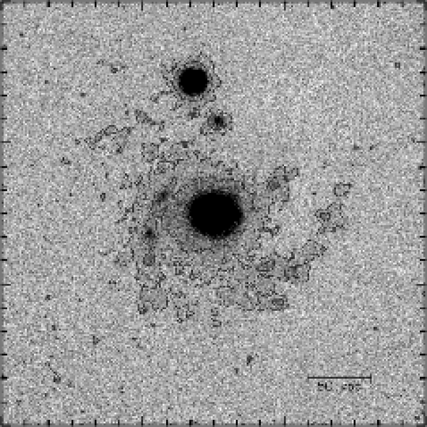
Figure 26: Deep H$\alpha$ image showing the extended nebular emission surrounding the quasar MR2251-178. The image was obtained by Shopbell, Veilleux & Bland-Hawthorn (1999) using the Taurus Tunable Filter. The frame is $3^{\prime}\times 2.5^{\prime}$ with north up and east to the left, and reaches a flux limit of $1.8\times 10^{-17}$ erg s^-1 cm^-2 arcsec^-2. The faint curved structure to the south-west is real and not a residual ghost image.

7 SUMMARY AND FUTURE PROSPECTS

In this review we have outlined the main principles behind Fabry-Perot detection and spectrophotometry from narrowband scans of Fabry-Perot data, with particular reference to low resolution tunable filter data. We have also discussed the most common limitations which need to be addressed for reliable photometric calibration. The imaging Fabry-Perot interferometer has the capability to provide superior spectrophotometry, since slit-aperture devices suffer seeing losses and narrowband filters are tacitly assumed to have constant transmission properties as a function of both position and wavelength. Fabry-Perot interferometers are still not common-user instruments at any observatory for a variety of reasons, most notably because of the restricted wavelength coverage. But for studying extended emission from a few bright lines, the capabilities of the Fabry-Perot are unmatched by any other technique, with the exception of the imaging Fourier Transform spectrometer. Figure 26 shows tunable filter imaging of the faint H$\alpha$ extended emission around the $z=0.0638$ quasar MR2251-178, obtained by Shopbell, Veilleux & Bland-Hawthorn (1999) using techniques described in this paper.

Fabry-Perot interferometers (including TTF) differ from an ideal tunable monochromator in three areas. First, the triangular rather than square shape of the Airy profile limits sampling efficiency and complicates flux calibration. A potential solution is the development of a ‘double cavity’ interferometer which squares the Lorentzian instrumental profile while maintaining high throughput (vand de Stadt & Muller 1985). Second, the use of fixed blocking filters limits the true tunable potential of the device. The use of two or more Fabry-Perot interferometers in series can bypass this restriction, thereby making a fully tunable system (Meaburn 1972). However, such a system comes at the cost of increased operating complexity. An intermediate solution is the use of custom-built rugate multiband blocking filters, transmitting two widely-separated intervals simultaneously (Cianci, Bland-Hawthorn & O’Byrne 2000). Finally, the phase change across the field presents a position-dependent passband that restricts the angular size of emission that can be imaged at any one time.

However, there are many promising technologies that look set to take tunable imaging beyond the Fabry-Perot interferometer. Acousto-optic tunable filters are an alternative where the active optical element comprises piezoelectric transducers bonded to an anisotropic birefringent material (Harris & Wallace 1969). An AC signal through the transducers (10-250 MHz), creates sonic waves that vibrate the crystal where it acts like a diffraction grating. Such tunable filters are currently limited by the expense and difficulty at manufacturing suitably-sized crystals of good imaging quality. The power to drive the vibrations is high (several watts per square centimetre) and there are difficulties concerning heat dissipation. Liquid crystal filters are an alternative technology that are now commercially produced, albeit with transmissions ($\sim 30$%) that remain too low for nighttime astronomical work. Solc filters (Solc 1959; Evans 1958) are tunable devices utilising a pair of polarisers with a sequence of phase retarders set to differing position angles. With a Solc filter it is possible to tune the shape of the spectral profile, in addition to its placement and dimensions.

The most advanced alternative tunable technique is that of the tunable Lyot filter, (Lyot 1944), consisting of many birefringent crystals in series. Birefringent filters cause incident light of two polarisation states to interfere with each other. The resulting bandpass is tuned by rotating all elements and its width is set by the thickness of the thinnest crystal. Such systems are already in wide use at solar observatories and we believe it will not be long before such systems find their way into nighttime work. The main drawback for astronomical use is that half the light is lost at the entrance polariser. The widefield tunable Lyot design of Bland-Hawthorn et al.  (2001) places such an arrangement at the prime focus of the telescope. Not only does this combat the light-loss problem, but it gives the filter access to wide sky angles (and short $f$-ratios) that would never be feasible with a Fabry-Perot instrument.

In the mean time, however, a low-order Fabry-Perot etalon such as TTF presents the best high-throughput system capable of tunable imaging.

References

Acker, A., Ochensenbein, F., Stenholm, B., Tylenda, R. Marcout, J., Mischon, C. 1992, The Strasbourg-ESO Catalogue of Galactic Planetary Nebulae (ESO: Garching)

Atherton, P. D., Reay, N. K., Ring, J., Hicks, T. R. 1981, Opt Eng 20, 806

Atherton, P. D., Reay, N. K., 1981, MNRAS 197, 507

Bacon, D. J., Refregier, A. R., Ellis, R. S. 2000, MNRAS 318, 625

Baker, J. C., Hunstead, R. W., Bremer, M. N., Bland-Hawthorn, J., Athreya, R. A. and Barr, J. 2001, AJ 121, 1821

Bertin, E., Arnouts, S. 1996, A&A 117, 393

Bessell, M. S. 1999, PASP 111, 1426

Bland, J., Tully, R. B. 1989, AJ 98, 723

Bland-Hawthorn, J., Shopbell, P. L., Cecil, G. 1992, in Astronomical Data Analysis: Software & Systems $-$ I, eds. D. Worrall, C. Biemsderfer, J. Barnes (ASP: San Francisco), p. 393

Bland-Hawthorn, J. 1995, in Tridimensional Optical Spectroscopic Methods in Astrophysics, ASP Conference Series Volume 71, eds. G. Comte, M. Marcelin (ASP: San Francisco), p. 72

Bland-Hawthorn, J., Jones, D. H. 1998a, PASA, 15, 44

Bland-Hawthorn, J., Jones, D. H. 1998b, in Optical Astronomical Instrumentation, Proc SPIE 3355, ed. S. D’Odorico, (SPIE: Bellingham, Washington), 855

Bland-Hawthorn, J., van Breugal, W., Gillingham, P. R., Baldry, I. K., Jones, D. H. 2001, ApJ accepted

Bookstein, F.L. 1979, Comp. Graph. & Image Proc., 9, 56

Cecil, G., 1988, ApJ 329, 38

Cianci, S. 2002, PhD Dissertation, University of Sydney, in prep.

Cianci, S., Bland-Hawthorn, J., O’Byrne, J. W. 2000, in Optical and IR Telescope Instrumentation and Detectors, Proc SPIE 4008, (SPIE: Bellingham, Washington), 1368

Deutsch, E.W., Margon, B., Bland-Hawthorn, J. 1998, PASP 110, 912

Evans, J. W.. 1958, J Opt Soc Amer 48, 142

Gander, W., von Matt, U. 1993, in Scientific Problems in Scientific Computing, eds. W. Gander & J. Hrebicek, (Springer-Verlag), p 251

Glazebrook, K., Bland-Hawthorn, J., 2001, PASP 113, 197

Haffner, L. M., Reynolds, R. J., Tufte, S. L. 1999, ApJ, 523, 223

Hamuy, M., Suntzeff, N. B., Heathcote, S. R., Walker, A. R., Gigoux, P., Phillips, M. M. 1994, PASP 106, 566

Harris, S. E., Wallace, R. W. 1969, J. Opt. Soc. Amer., 59, 744

Jacquinot, P. 1954, J Opt Soc Amer 44, 761

Jacquinot, P. 1960, Rep Prog Phys 23, 267

Jones, D. H., Bland-Hawthorn, J. 2001, ApJ 550, 593

Jones, D. H 1999, PhD Dissertation, Australian National University

Jones, D. H., Bland-Hawthorn, J. 1998, PASP 110, 1059

Joseph, S. H. 1994, Comp Graph & Image Proc, 56, 424

Laval, A., Boulesteix, J., Georgelin, Y. P., Georgelin, Y. M., Marcelin, M. 1987, A&A, 175, 199

Lissberger, P. H., Wilcock, W. L. 1959, J Opt Soc Amer 49, 126

Lyot, B. 1944, Ann. d’Ap., 7, 31

Meaburn, J. 1972, A&A 17, 106

Meaburn, J. 1976, Detection and Spectrometry of Faint Light, Dordrecht: Reidel

Rhoads, J. E. 2000, PASP 112, 703

Roesler, F. L. 1974, Meth Expt Phys, 12A, chap. 12

Shopbell, P. L., Bland-Hawthorn, J. 1998, ApJ 493, 129

Shopbell, P. L., Veilleux, S., Bland-Hawthorn, J. 1999, ApJ 524, L83

Stilburn, J. R. 2000, in Optical and IR Telescope Instrumentation and Detectors, Proc SPIE 4008, eds. M. Iye, A. F. Moorwood, (SPIE: Bellingham, Washington), 1361

Solc, I. 1959, Czech J Phys, 9, 237

Stevenson, C. C. 1994, MNRAS 267, 904

Taylor, K., Atherton, P. D. 1980, MNRAS 191, 675

Thorne, A. P. 1988, Spectrophysics, Chapman & Hall, London

Tinney, C. G., Tolley, A. J 1999, MNRAS 304, 119

Valdes, F. 1993, FOCAS User’s Guide, NOAO

van de Stadt, H., Muller, J. M. 1985, J. Opt. Soc. Am. A 2, 1363

Veilleux, S., Bland-Hawthorn, J., Cecil, G.,  1999, AJ 118, 2108

A Fitting Night-Sky Rings

Circular Fitting: Given three well-separated positions $(x_{1},y_{1})$, $(x_{2},y_{2})$ and $(x_{3},y_{3})$ along the ring, the centre $(x,y)$ can be found by solving the determinant

$$\left|\begin{array}[]{cccc}x^{2}+y^{2}&x&y&1\\ x_{1}^{2}+y_{1}^{2}&x_{1}&y_{1}&1\\ x_{2}^{2}+y_{2}^{2}&x_{2}&y_{2}&1\\ x_{3}^{2}+y_{3}^{2}&x_{3}&y_{3}&1\\ \end{array}\right|=0.$$ (A1)

Elliptical Fitting: For an ellipse centred on the origin, we write

$${\bf x}^{T}A{\bf x}+{\bf b}^{T}{\bf x}+c=0$$ (A2)

for which $A$ is symmetric and positive definite. Here, we have introduced a coordinate vector ${\bf x}=(x_{i1},x_{i2})^{T}$. In order to derive a form invariant under transformation, we replace ${\bf x}$ with $G{\bf x}+{\bf h}$. This leads to a similar form to Eqn. (A2) where $A$ is replaced by $G^{T}AG$, ${\bf b}$ becomes $(2{\bf h}^{T}A+{\bf b}^{T})G$, and $c$ is replaced by ${\bf h}^{T}A{\bf h}+{\bf b}^{T}{\bf h}+c$.

The eigenvalues $(\lambda_{1},\lambda_{2})$ for $A$ are obtained from a suitable choice of $G$ ($G^{T}G=1$), and ${\bf h}$ can be chosen to ensure ${\bf h}^{T}A{\bf h}+{\bf b}^{T}{\bf h}+c=0$. It follows that

$$\lambda_{1}{\bf x_{1}}^{2}+\lambda_{2}{\bf x_{2}}^{2}+c=0$$ (A3)

where $c$ is defined in the transformed frame. This is the equation of an ellipse subject to $(\lambda_{1}>0,\lambda_{2}>0,c<0).$ Since $A$ has the same real eigenvalues before and after transformation, all functions of the eigenvalues are invariant under transformation.

The eigenvalues share an important relationship with the coefficients of $A$, i.e.

$$\lambda_{1}\lambda_{2} = A_{11}A_{22}-A_{21}A_{12}\ \ \ ({\rm det~{}A})$$ (A4)

$$\lambda_{1}+\lambda_{2} = A_{11}+A_{22}\ \ \ ({\rm trace~{}A})$$ (A5)

$$\lambda_{1}^{2}+\lambda_{2}^{2} = A_{11}^{2}+2A_{12}+A_{22}^{2}$$ (A6)

Moreover, the geometric properties of the ellipse before transformation are

$$\alpha = \sqrt{-c/\lambda_{1}}$$ (A7)

$$\beta = \sqrt{-c/\lambda_{2}}$$ (A8)

where $(\alpha,\beta)$ are the semi-major axes; ${\bf h}$ defines the origin of the ellipse.

Finally, once each of the $p$ data points are placed in Eqn. (A2), we arrive at a highly overdetermined, nonlinear system of $p$ equations in the 4 unknown geometric parameters. This is a standard problem which can be solved efficiently with any number of gradient search algorithms subject to a constraint. The restriction needs to be invariant to the coordinate transformation: simply setting one of the unknowns to unity is not normally sufficient to ensure convergence. Two useful constraints (everywhere non-zero) are $\lambda_{1}+\lambda_{2}=1$ (Gander & von Matt 1993) and $\lambda_{1}^{2}+\lambda_{2}^{2}=1$ (Bookstein 1979).

It is important that the method, e.g. Levenberg-Marquardt, be efficient since $p\sim 10^{3}$ typically in TTF analysis. There are several possible weighting schemes which have varying merits for different data sets. The most common is flux weighting to ensure the fitting establishes the major axes (radius) as accurately as possible.

B Ghost Families

Internal reflections constitute a challenge for all optical systems, particularly imagers with dispersing optics at the pupil, such as tunable filters and Wollaston prisms. Even a minimal arrangement can have eight or more optically flat surfaces (e.g. blocking filter, CCD window). At some level, all of these surfaces interact separately to generate spurious reflections.

The periodic behaviour of the tunable filter always requires that we use an interference filter somewhere in the optical path, to block light from extraneous orders. The filter introduces ghost reflections within the Fabry-Perot optics. Such a filter placed in the converging beam before the collimator or after the camera lens generates a distinct pattern of diametric ghosts. A filter placed in the collimated beam has its own distinct family of exponential ghosts which are the most difficult to combat. The pattern of ghosts imaged at the detector is different in both arrangements, as illustrated in Fig. B2. Examples of the appearance of such ghosts are shown in Fig. B4.

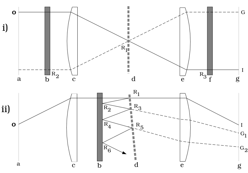
Figure B2: Ghost families arising from internal reflections within a Fabry-Perot spectrometer. ($i$) Diametric ghosts. Rays from the object O form an inverted image I and an out-of-focus image at R₃. The reflection at R₁ produces an out-of-focus image at R₂. The images at R₂ and R₃ appear as a ghost image G at the detector. ($ii$) Exponential ghosts. The images at R₂ and R₄ appear as ghost images G₁ and G₂ respectively.

Another ghost family arises from the down-stream optical element (extraneous etalon effect). The large optical gap of the outer plate surfaces produces a high-order Airy pattern at the detector. It is possible to suppress this signal by wedging the outer surfaces. However, if we are forced to operate the blocking filters in the collimated beam, this compounds the problem further.

To a large extent, we can minimize the impact of diametric and exponential ghosts through the use of well-designed anti-reflection coatings. The reflectivity $r$ of an air-glass interface is

$$r=\frac{(\mu_{\rm glass}-\mu_{\rm air})^{2}}{(\mu_{\rm glass}+\mu_{air})^{2}}=4\%$$ (B1)

where $\mu_{\rm glass}\approx 1.5$ and $\mu_{\rm air}=1.0$. This can be significantly reduced to 1% or better by the application of an AR coating (half-optical band), or to below 0.1% for AR coatings customized to the particular filter in question. Coating performance is currently limited by the availability of pure transparent dielectrics with high refractive indices. A promising alternative is the use of silica sol-gel coatings, that reduce the reflective losses inherent with traditional MgF₂ coatings (Stilburn 2000). The durability of these coatings has been improved over recent years to the point where they are now being routinely used on instruments for 4 and 8 m-class telescopes with many air-glass surfaces.

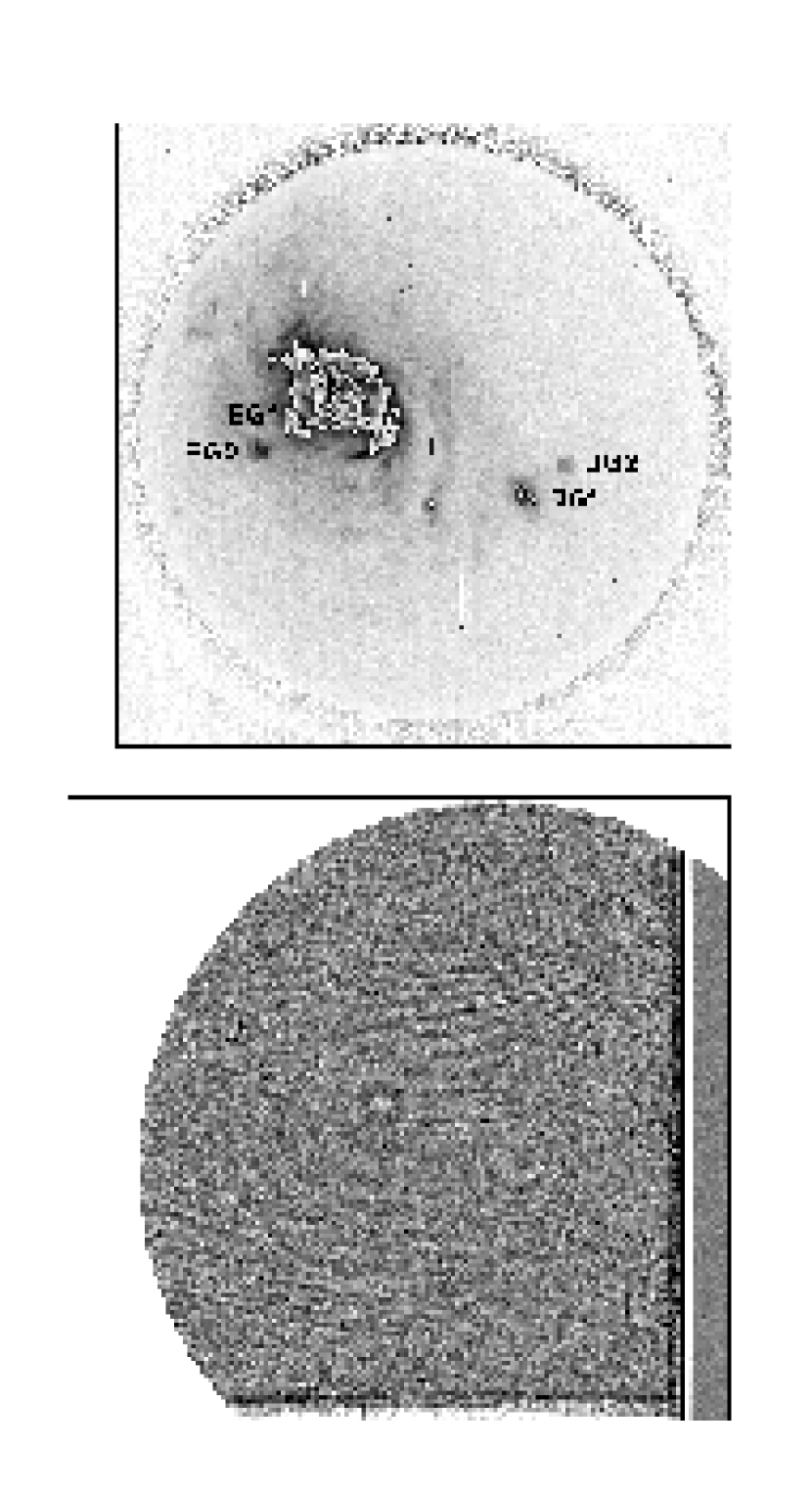
Figure B4: Top.- Two ghost families are seen in this image of NGC 1068 taken with the Rutgers Fabry-Perot on the CTIO 4.0 m telescope. The optical axis is indicated by the cross. N is placed slightly to the north of the Seyfert nucleus. DG1 is the diametric ghost of the active nucleus; EG1 is an exponential ghost of the Seyfert nucleus. DG2 is the diametric ghost of EG1 and EG2 is the exponential ghost of EG1. Bottom.- The ‘extraneous etalon’ ghost pattern from the downstream etalon plate (lower right quadrant) and from an air gap in the MOSFP camera (central). The data were taken at the CFHT by illuminating the dome with an H$\alpha$ lamp. The fringe pattern of the Loral #3 CCD has a similar peak to trough amplitude.

A more difficult reflection problem arises from the optical blanks which form the basis of the etalon. These can act as internally reflecting cavities since, from Sect. 3.1, if we let ${\cal R}_{1}=0.96$ and ${\cal R}_{2}={\cal AR}_{1}=0.04$ (air-glass), it generates a ripple pattern with a finesse close to unity. The large optical gap of the outer plates produces a high-order Airy pattern at the detector (Fig. B4). Traditionally, the outer surfaces have been wedge-shaped to deflect this spurious signal out of the beam. However, if the surfaces are not coated with suitable anti-reflection coatings then the problem is compounded by an additional set of ghosts (Fig. B6). These spurious reflections diverge as a result of the wedge angle. Furthermore, reflections from the front plate only occur for monochromatic sources, thereby complicating identification in fields containing both stars and emission-line sources.

Even after we have paid full attention to minimizing air-glass reflections, there remains one fundamental ghost arising from the CCD. As we see from the equation above, silicon ($\mu_{\rm Si}=3.5$) leads to an air-silicon reflection of 30%. A modern prescription broadband AR coating for a CCD reduces this by a factor of 3, meaning that ghosts reside at around 10%. Since we cannot customize the CCD response for a narrow wavelength range, bright ‘in-focus’ diametric ghosts must always occur with a tunable filter imager. A good way to track these down is to place a regular grid of holes in focus at the focal plane and illuminate the optical system with a whitelight source (Sect. 4.2), tilting the etalon such that ghost images of the grid avoid the detector area. If tilting is not possible, then dithering and median filtering are required, (Sect. 5.3).

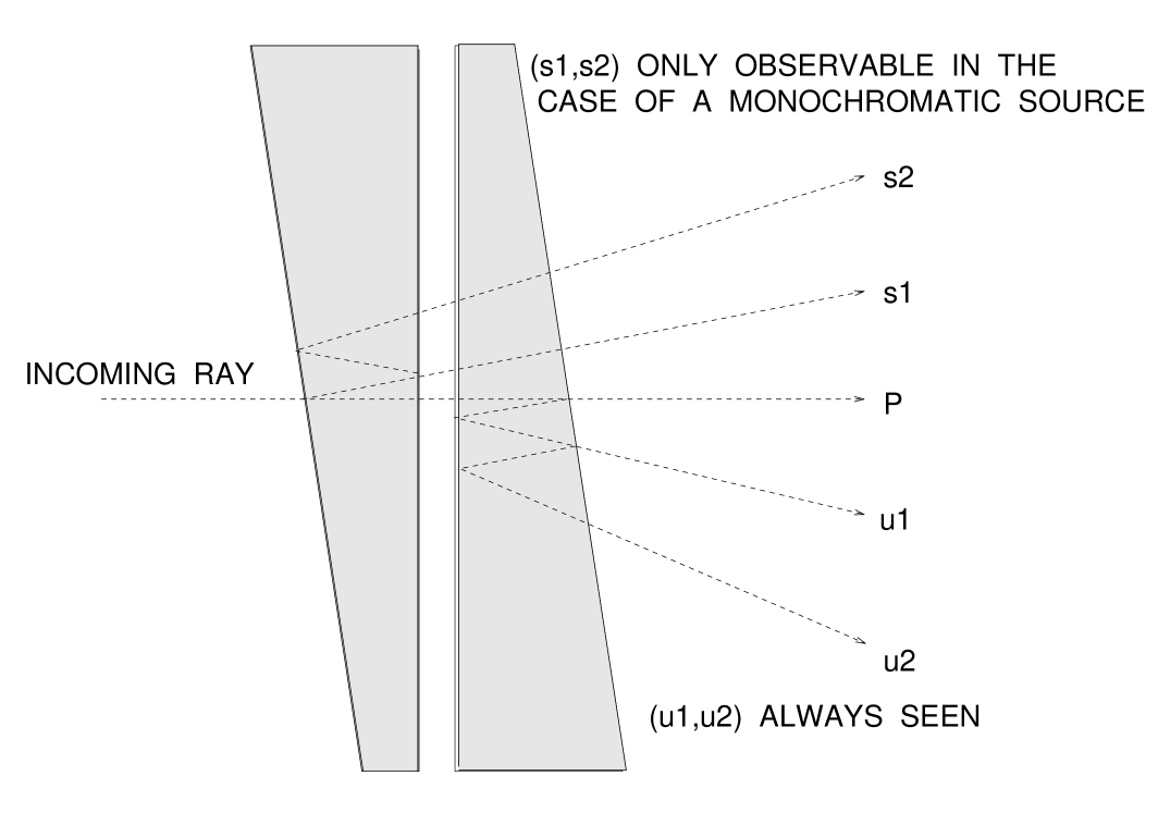
Figure B6: The diverging ghost families arising from wedged Fabry-Perot plates with poor anti-reflection coatings on the outer surfaces.

C Weak Cosmic Rays

Here, we describe a simple test to evaluate the effectiveness of any software in removing weak cosmic-ray events. The method is to compare the probability distribution function (PDF) of cosmic ray events between an observation and a dark frame matched in exposure time. We illustrate the basic idea using dark exposures from a Tektronix $1024\times 1024$ CCD with varying exposure lengths and read-out times.

We used the Tekronix CCD at the AAT 3.9 m with varying exposure lengths (15, 30, 60, 120 min) and read-out times (FAST, SLOW, XTRASLOW). The histogram of each frame shows the contribution from the bias, read and dark noise. A millisecond exposure was used to remove the bias and read noise contribution to each histogram. The additional contribution from the dark noise was well calibrated at 0.11 cts pix^-1 ksec^-1. It is assumed that the remaining events are related to cosmic rays.

We define $n(E)\ dE$ to be the number of cosmic ray events with energies (expressed in counts) in the range $(E,E+dE)$. The cumulative distribution is then

$$P(E)=\int_{0}^{E}n(E)\ dE$$ (C1)

When $n(E)\propto E^{\beta}$, the slope of the plot $\log P$ vs. $\log E$ is proportional to $\beta+1$. In Fig. C2 (top), the noisy histogram is the bias/dark/read noise subtracted dark frame. The monotonic curve is a plot of $\log P$ vs. $\log E$ which is found to be rather well defined and reproducible over the different exposures. The PDF for the data is determined from all events identified by the deglitch algorithm. Since the energetic events are easier to find, the bright end of both PDFs will be well matched. In Fig. C2 (bottom), where the deglitch PDF turns over at low energy — presumably but not necessarily at an energy greater than or equal to the turnover in the dark PDF — gives some idea as to how effective the algorithm has been in removing the weaker events.

Figure C2: Top. Histogram of cosmic ray events in a two hour dark frame. The monotonic curve is the cumulative histogram of these events. The error bars are Poissonian and not independent. Bottom. The cumulative histogram from above with which to compare the performance of a deglitch algorithm. Three cases are illustrated: algorithm A is too conservative, algorithm B more reliable, and algorithm C has mistaken real data with faint cosmic rays.

	$f(x)$	$\int f(x)\ dx$
G	$\exp[-\ln 16\ {\rm mod}[x,\Delta x]^{2}/(\delta x)^{2}]$	$({{\delta x}\over 2})\sqrt{{\pi\over{\ln 2}}}\;{\rm erf}[({{2\sqrt{\ln 2}}\over{\delta x}})\ {\rm mod}[x,\Delta x]]$
L	$(1+({2\over{\delta x}})^{2}\ {\rm mod}[x,\Delta x]^{2})^{-1}$	$({{\delta x}\over 2})\ \tan^{-1}[({2\over{\delta x}})\ {\rm mod}[x,\Delta x]]$
A	$(1+\alpha\sin^{2}({{\pi x}\over{\Delta x}}))^{-1}$	$({{\Delta x}\over{\pi\sqrt{1+\alpha}}})\ \tan^{-1}[\sqrt{1+\alpha}\ \tan({{\pi x}\over{\Delta x}})]$

Table 2: Cyclic functions which are periodic over $\Delta x$ with FWHM $\delta x$. The (G)aussian, (L)orentzian and (A)iry functions are illustrated in Fig. 6. The mod function is the modulo function and $\alpha=({{2\ \Delta x}\over{\pi\ \delta x}})^{2}$. Note that for large $\alpha$, $({{\Delta x}\over{\pi\sqrt{1+\alpha}}})\approx({{\delta x}\over 2})$. The gap scanning variable $x$ is offset by ${{\Delta x}\over{2}}$ in practice.

Source	Useful Range
	(nm)
zinc	308 – 636
thallium	352 – 535
mercury-cadmium	370 – 450
deuterium-helium	450 – 550†
cesium	456 – 921
neon	500† – 700
copper-argon	700 – 1000

Table 4: Arc lamps used for wavelength calibration of the tunable filter system at the AAT, showing the range of wavelengths over which they are useful. $\dagger$ For calibrations around 500 nm, the astrophysical lines H$\beta$ $\lambda$4861 and [O iii] $\lambda\lambda$4959,5007 found in planetary nebulae (Acker et al.  1992) may be more suitable.