ABBOTT WAVE-TRIGGERED RUNAWAY IN LINE-DRIVEN WINDS FROM STARS AND ACCRETION DISKS

Abstract

Line-driven winds from stars and accretion disks are accelerated by scattering in numerous line transitions. The wind is believed to adopt a unique critical solution, out of the infinite variety of shallow and steep solutions. We study the inherent dynamics of the transition towards the critical wind. A new runaway wind mechanism is analyzed in terms of radiative-acoustic (Abbott) waves which are responsible for shaping the wind velocity law and fixing the mass loss. Three different flow types result, depending on the location of perturbations. First, if the shallow solution is perturbed sufficiently far downstream, a single critical point forms in the flow, which is a barrier for Abbott waves, and the solution tends to the critical one. Second, if the shallow solution is perturbed upstream from this critical point, mass overloading results, and the critical point is shifted inwards. This wind exhibits a broad, stationary region of decelerating flow and its velocity law has kinks. Third, for perturbations even further upstream, the overloaded wind becomes time-dependent, and develops shocks and dense shells.

Submitted to the Astrophysical Journal

and

1 Introduction

Radiation-driven winds which are accelerated by absorption and re-emission of continuum photons in spectral lines form an interesting class of hydrodynamic flows, termed line-driven winds (LDWs). They occur in OB and W-R stars, cataclysmic variables, and probably in active galactic nuclei and luminous young stellar objects. These winds are characterized by a unique dependence of line force on the velocity gradient in the flow. This causes a new, radiative wave type.

The nature of these waves was first discussed by Abbott (1980, hereafter ‘Abbott waves’), who found two modes, a slow, acoustic one propagating downstream, and a fast, radiative one propagating upstream. The critical point found by Castor, Abbott, & Klein (1975, hereafter CAK) from analysis of the stationary Euler equation is a barrier for these waves, the same way as the sonic point is to sound waves. The intriguing property of Abbott waves is that they propagate downstream slower than the sound speed, while they propagate upstream at very large speeds, highly supersonically. The latter fact reflects essentially the radiative nature of Abbott waves.

No such upstream propagating, radiative mode was found by Owocki & Rybicki (1986), who calculated the Green’s function for winds driven by pure line absorption. The explanation is that the pure absorption case suppresses the radiative upstream mode, as photons can propagate only downstream. The radiative upstream mode is back when line scattering is included (Owocki & Puls 1999).

The question arises for the physical interpretation of Abbott waves. Do they represent a physical entity which is responsible for shaping the flow by communicating essential flow properties between different points in the wind? In particular, could Abbott waves be the prime cause for evolution of LDWs towards a CAK-type, steady-state solution?

The analysis by CAK of the steady-state Euler equation for LDWs has revealed an infinite family of mathematical solutions, but only one, hereafter ‘critical solution,’ which extends from the photosphere to arbitrary large radii. Other solutions either do not reach infinity or the photosphere. The former solutions are called shallow and the latter ones — steep. The unique, critical wind starts as the fastest shallow solution and switches smoothly to the slowest steep solution at the critical point.

The shallow wind solutions found by CAK are the analog to solar wind breezes, in that they are sub-abbottic everywhere. They were abandoned by CAK because they cannot provide the required spherical expansion work at large radii. This exclusion of shallow solutions can be criticized in different respects: (i) the breakdown happens only around 300 stellar radii, where basic assumptions of the model (fluid description; spherical symmetry; isothermality) may become invalid. (ii) Shallow solutions could be extended to infinity by jumping at some large radius to a decelerating wind branch. The latter was excluded a priori by CAK. However, this jump can occur beyond a few stellar radii, where the wind has already reached its local escape speed. (iii) For models of disk LDW, even the critical solution itself does not extend to infinity, and becomes imaginary beyond a certain radius (Feldmeier & Shlosman 1999). Jumps to the decelerating branch are unavoidable then.

With shallow solutions being valid stationary solutions, the question arises, what forces the wind to adopt the critical CAK solution? Numerical aspects of this question have been discussed by Feldmeier, Shlosman & Hamann (2001), who noted that outer boundary conditions and a Courant time step which do not account for Abbott waves can set off numerical runaway, often towards the critical solution.

In the present paper, we focus on a physical interpretation of Abbott waves, extending our previous work on this subject (Feldmeier & Shlosman 2000). We show that these waves are the prime driver of evolution of LDWs towards a unique, steady-state solution characterized by a specific velocity law and mass loss rate. In particular, we find that as is the case for solar wind breezes, shallow solutions can evolve due to waves which propagate upstream to the wind base (the photosphere). As a new effect in LDWs, Abbott waves ‘drag’ the solution in one preferred direction, towards larger velocities. The wind becomes stable when a critical point forms, through which outer perturbations can no longer penetrate inwards.

2 Abbott waves

2.1 Wind model

Only wind acceleration due to a line force in Sobolev approximation for radiative transfer is considered in this paper. The large number of lines driving the wind is dealt with using a CAK line distribution function. The latter is characterized by a power law index $\alpha$, which lies between 0 and 1. The Sobolev force is proportional to

$$g_{\rm l}\sim\int d\omega\,{\bf n}I_{\bf n}\tau_{\bf n}^{-\alpha},$$ (1)

where ${\bf n}$ is the unit vector pointing in the direction of the surface angle element $d\omega$, $I$ is the frequency integrated specific intensity, and $\tau$ is the Sobolev optical depth,

$$\tau_{\bf n}={\kappa\rho v_{\rm th}\over{\bf n}\cdot({\bf n}\cdot(\nabla{\bf v}))},$$ (2)

with rate-of-strain tensor $\nabla{\bf v}$, mass absorption coefficient $\kappa$, and ion thermal speed $v_{\rm th}$. The force proportionality constant is fixed later in terms of the critical solution. Through $\nabla{\bf v}$, the line force depends on the streamline geometry. To simplify, we take $\tau$ in (1) out of the integral and replace it by an average or equivalent optical depth in one direction. Specifically, the latter is assumed to be the flow direction. This approach corresponds to the CAK ‘radial streaming approximation.’ For a planar flow with height coordinate $z$, the line force becomes, assuming constant $\kappa$ and $v_{\rm th}$,

$$g_{\rm l}\sim F(v^{\prime}/\rho)^{\alpha},$$ (3)

where $v^{\prime}=\partial v/\partial z$, and the radiative flux $F$ is a function of $z$. Even this highly idealized line force depends in a non-linear way on the hydrodynamic variables $v^{\prime}$ and $\rho$.

So far, the following assumptions were introduced: (i) the line force is calculated in Sobolev approximation, using (ii) a CAK line distribution function (without line overlap), and (iii) applying the radial streaming approximation for (iv) planar flow. To these, we add the further assumptions: (v) the flux $F$ is constant with $z$, but gravity $g$ may depend arbitrarily on $z$. This can serve to model winds from thin, isothermal accretion disks, in which case $g$ grows first linearly with $z$ and at large distances drops off as $z^{-2}$. Alternatively, with $F$ and $g$ being constants, one can model the launch region of a stellar wind, but a well-known degeneracy occurs here (Poe, Owocki, & Castor 1990). (vi) Zero sound speed is assumed, $a=0$, and (vii) we fix $\alpha=1/2$. Note that the Sobolev line force is independent of $v_{\rm th}$ and therefore of $a$. LDWs are hypersonic, and except near the photosphere, gas pressure plays no role. The 1-D continuity and Euler equations are,

$${\partial\rho\over\partial t}+v{\partial\rho\over\partial z}+\rho{\partial v\over\partial z}=0,$$ (4)

$$E\equiv{\partial v\over\partial t}+v\,{\partial v\over\partial z}+g(z)-C_{0}\,F\sqrt{{\partial v/\partial z\over\rho}}=0,$$ (5)

with constant $C_{0}$. We consider first stationary solutions, $\rho v={\rm const}$. A normalized quantity $m=\rho v/\rho_{\rm c}v_{\rm c}$ is introduced, where $\rho_{\rm c}(z)$ and $v_{\rm c}(z)$ are the density and velocity law of the critical wind, which is defined below. Besides $m$, a second, new hydrodynamic variable, $w^{\prime}=vv^{\prime}$, is defined, and the Euler equation becomes,

$$w^{\prime}+g(z)-C\sqrt{w^{\prime}/m}=0.$$ (6)

The flux $F$ was absorbed into the constant $C$. At each $z$, (6) is a quadratic equation in $\sqrt{w^{\prime}}$, with solutions,

$$\sqrt{w^{\prime}}={1\over 2\sqrt{m}}\left(C\pm\sqrt{C^{2}-4gm}\right).$$ (7)

The velocity law $v(z)$ is obtained from $w^{\prime}$ by quadrature. Solutions with ‘$-$’ are termed shallow, those with ‘$+$’ are termed steep. If $m<1$ (see below), shallow and steep solutions exist from $z=0$ to $\infty$. If $m>1$, shallow and steep solutions become imaginary in a certain $z$ interval. In this region, the line force $\sim C/\sqrt{m}$ cannot balance gravity $g$.

Within the family of shallow wind solutions, the mass flux $\rho v$ increases monotonically with terminal speed, while for steep solutions the trend is opposite. The largest mass flux which keeps the solution everywhere real defines the critical wind, $m_{\rm c}=1$. Setting the square root in eq. (7) to 0, this implies for $C$,

$$C=2\sqrt{g_{\rm c}},$$ (8)

where $g_{\rm c}=g(z_{\rm c})$ means gravity at the critical point of the critical solution. How is $z_{\rm c}$ found? Differentiating the stationary Euler equation, $E\bigl{(}z,w^{\prime}(z)\bigr{)}=0$, with respect to $z$ and using $\partial E/\partial w^{\prime}_{\rm c}=0$ at the critical point (crossing of solutions), one finds

$$0={dE\over dz_{\rm c}}={dg\over dz_{\rm c}}.$$ (9)

Hence, the critical point coincides with the gravity maximum. This is not an accident, but expresses that the critical point lies at the bottleneck of the flow, as for a Laval nozzle (Abbott 1980). If the flux $F$ varies with $z$, the generalized area function depends also on $F$, and the critical point no longer coincides with the gravity maximum (see Feldmeier & Shlosman 1999 for examples). If $g={\rm const}$, the critical point degenerates, and every point in the flow becomes critical. In stellar wind calculations, the correct critical point location is found by including the finite cone correction factor for the stellar disk as an ‘area’ function (Pauldrach, Puls, & Kudritzki 1986; Friend & Abbott 1986).

The wind solution becomes,

$$w^{\prime}={g_{c}\over m}\left(1\pm\sqrt{1-{mg\over g_{c}}}\right)^{2}.$$ (10)

At the critical point, shallow and steep solutions with $m=1$ merge in such a way that the slope in passing from one to the other is continuous. Staying instead on either shallow or steep solutions introduces a discontinuity in $v^{\prime\prime}(z_{\rm c})$. Discontinuities in derivatives of hydrodynamic variables, termed weak discontinuities, lie on flow characteristics (Courant & Hilbert 1968). Characteristics are the space-time trajectories of wave phases. Indeed, we find below that the critical point is a barrier for Abbott waves.

It is at this point that the question arises, which solution the wind adopts — a shallow, steep, or critical one. This issue will be resolved by discussing runaway of shallow solutions. We shall find that Abbott waves are the prime driver of this evolution.

2.2 Green’s function

We derive the Green’s function for Abbott waves in Sobolev approximation. The Green’s function gives the response of a medium to a localized, delta function perturbation in space and time, and is complementary to the harmonic dispersion analysis of Abbott (1980) and Owocki & Rybicki (1984). Since localized perturbations contain many harmonics, a Green’s function describes wave interference. This is clearly seen for surface water waves, whose Green’s function is known from Fresnel diffraction in optics (Lamb 1932, p. 386). For simplicity, we consider only a single, optically thick line, with Sobolev force ($\alpha\equiv 1$),

$$g_{\rm l}=A\;{\partial v\over\partial z}.$$ (11)

Density $\rho$ was absorbed into the constant $A$. We assume WKB approximation to hold (slowly varying background flow) and consider velocity perturbations only. The characteristic analysis in the next section will show that the Abbott wave amplitude is $v^{\prime}/\rho$, hence, Abbott waves are not annihilated by this restriction to velocity perturbations. The linearized Euler equation for small perturbations is

$${\partial\over\partial t}\delta v(z,t)=\delta g_{\rm l}(z,t)=A\,\delta v^{\prime}(z,t).$$ (12)

The Green’s function problem is posed by specifying as initial conditions,

$$\delta v(z,0)=\delta(z-z_{0}).$$ (13)

Multiplying eq. (12) by $e^{-ikz}$ and integrating over $z$,

$${\partial\over\partial t}\overline{\delta v}(k,t)=ikA\overline{\delta v}(k,t),$$ (14)

where a bar indicates Fourier transforms, $\overline{\delta v}=$ $\int\delta v$ $e^{-ikz}dz$. The right hand side was obtained by integration by parts, assuming $\delta v(-\infty,t)=\delta v(\infty,t)=0$. This is shown a posteriori. The solution of (14) is

$$\overline{\delta v}(k,t)=be^{ikAt},$$ (15)

with constant $b$. Fourier transforming (13) from $z$ to $k$ space,

$$\overline{\delta v}(k,0)=e^{-ikz_{0}}=b,$$ (16)

and

$$\overline{\delta v}(k,t)=e^{ik(At-z_{0})}.$$ (17)

Fourier transforming back to $z$ space,

$$\delta v(z,t)={1\over 2\pi}\int_{-\infty}^{\infty}dk\,e^{ikz}e^{ik(At-z_{0})}=\delta(z-z_{0}+At).$$ (18)

Therefore, the initial delta function propagates without dispersion towards smaller $z$, at an Abbott speed $-A$. Furthermore, $\delta v=0$ at $z=\pm\infty$, as assumed. Since no wave dispersion occurs, the same Abbott speed $A$ is also obtained by considering harmonic perturbations. Inserting $\delta v=\overline{\delta v}\,e^{i(kz-\omega t)}$ in (12) gives as phase and group speed,

$${\omega\over k}={d\omega\over dk}=-A.$$ (19)

The Green’s function, $G$, is defined by ($F$ an arbitrary function),

$$F(z,t)=\int_{-\infty}^{\infty}dz^{\prime}\,G(z-z^{\prime},t)\,F(z^{\prime},0).$$ (20)

From (13) and (18),

$$G(z,t)=\delta(z+At),$$ (21)

a result first obtained by Owocki & Rybicki (1986).

The present case of optically thick lines only corresponds to $\alpha=1$. An explicit expression for the Abbott speed is not relevant then: opposed to all cases $\alpha<1$, $\alpha=1$ poses no eigenvalue problem for $m$. We return therefore to $\alpha=1/2$.

2.3 Abbott wave characteristics

Besides a harmonic and Green’s function analysis, a characteristic analysis can be given for Abbott waves. Especially, the latter is not restricted to linear waves. Inserting $C$ from (8), the equations of motion (4, 5) become (dots indicate time derivatives),

$$\dot{\rho}+v\rho^{\prime}+\rho v^{\prime}=0,$$ (22)

$$\dot{v}+v\,v^{\prime}+g(z)-2\Gamma\sqrt{v^{\prime}\over\rho}=0,$$ (23)

where we introduced the constant

$$\Gamma=\sqrt{g_{\rm c}\rho_{\rm c}v_{\rm c}}.$$ (24)

To bring these equations into characteristic form, we first write the continuity equation formally as $K(\rho,v)=0$, the Euler equation as $E(\rho,v)=0$. For non-linear, first order systems of partial differential equations, $K=0$ and $E=0$, in two unknown variables $\rho$ and $v$, the latter being functions of coordinates $t$ and $z$, the characteristic directions or speeds, $a$, are determined by (Courant & Hilbert 1968; vol. II, chap. 5, §3)

$$\begin{vmatrix}-aK_{\dot{\rho}}+K_{\rho^{\prime}}&-aK_{\dot{v}}+K_{v^{\prime}}\\ -aE_{\dot{\rho}}+E_{\rho^{\prime}}&-aE_{\dot{v}}+E_{v^{\prime}}\end{vmatrix}=0,$$ (25)

where $K_{\rho^{\prime}}=\partial K/\partial\rho^{\prime}$, $E_{\dot{v}}=\partial E/\partial\dot{v}$, etc. We use the symbol $a$, hitherto reserved for the sound speed, also for characteristic speeds. The meaning should be clear from the context. Inserting $K$ and $E$ in (25),

$$\begin{vmatrix}-a+v&\rho\\ 0&-a+v-{\displaystyle\Gamma\over\displaystyle\sqrt{\rho v^{\prime}}}\end{vmatrix}=0,$$ (26)

hence,

$$a_{+}=v,\qquad a_{-}\equiv A=v-{\Gamma\over\sqrt{\rho v^{\prime}}},$$ (27)

in the observers frame. The Abbott speed is again denoted $A$. In the comoving frame, $a_{+}=0$ and $a_{-}=-\Gamma/\sqrt{\rho v^{\prime}}$. The downstream ($+$), slow wave mode corresponds to sound waves. The upstream ($-$), fast mode is of radiative origin.

A simple, heuristic argument can be given for the occurence of Abbott waves. Consider a long scale perturbation of a stationary velocity law. At the node where the velocity gradient gets steepened, the Sobolev line force increases. The gas is accelerated to larger speeds, hence the node shifts inwards. Similarly, the node where the velocity law becomes shallower shifts inwards. The node shift corresponds to phase propagation of a harmonic wave.

Next, we bring the equations of motion into characteristic form. To this end, the Euler equation is quasi-linearized by differentiating it with respect to $z$ (Courant & Hilbert 1968), introducing a new, fundamental variable $f=v^{\prime}$,

$$\dot{f}+vf^{\prime}+f^{2}-{\Gamma\over\sqrt{f\rho}}\left(f^{\prime}-f{\rho^{\prime}\over\rho}\right)+g^{\prime}=0.$$ (28)

Re-bracketing and multiplying with $\rho$,

$$\rho\dot{f}+\rho Af^{\prime}+\rho f^{2}+{\Gamma\over\sqrt{f\rho}}f\rho^{\prime}+\rho g^{\prime}=0.$$ (29)

Using the continuity equation,

$$0 =\rho\dot{f}+\rho Af^{\prime}-f\dot{\rho}-\left(v-{\Gamma\over\sqrt{f\rho}}\right)f\rho^{\prime}+\rho g^{\prime}$$

$$=\rho\dot{f}+\rho Af^{\prime}-f\dot{\rho}-Af\rho^{\prime}+\rho g^{\prime}$$ (30)

$$=\rho^{2}\left(\partial_{t}+A\partial_{z}\right){f\over\rho}+\rho g^{\prime}.$$

The Euler equation in characteristic form is therefore,

$$\left(\partial_{t}+A\partial_{z}\right){v^{\prime}\over\rho}=-{g^{\prime}\over\rho},$$ (31)

with $A$ from (27). We assume that WKB approximation applies, i.e., that the temporal and spatial derivatives on the left hand side are individually much larger than the right hand side, hence the latter can be neglected. In a frame moving at speed $-A$, the function $v^{\prime}/\rho$ is constant, and can be interpreted as a wave amplitude. Note that $v^{\prime}/\rho$ is inversely proportional to the Sobolev line optical depth, indicating that Abbott waves are indeed a radiative mode.

Introducing $f$ in the continuity equation puts it into characteristic form,

$$\left(\partial_{t}+v\partial_{z}\right)\rho=-f\rho.$$ (32)

Here, $f\rho$ is an inhomogeneous term. WKB approximation cannot be assumed here, since $f$ may vary on short scales. The wave amplitude, $\rho$, is no longer constant along $v$ characteristics, but changes according to this (ordinary) differential equation. Since gas pressure $p$ scales with density, this equation shows that the outward mode corresponds to sound.

For stationary winds, the Abbott speed in the observers frame becomes ($\alpha=1/2$),

$$A=v\left(1-\sqrt{g_{c}\over mw^{\prime}}\right)=v\left(1-{1\over\sqrt{mw^{\prime}/w^{\prime}_{c}}}\right),$$ (33)

since $w_{\rm c}^{\prime}=g_{\rm c}$ from (7, 8). With $A_{\rm c}=0$, the critical point is a stagnation point for Abbott waves. For shallow winds, $m<1$ and $w^{\prime}/w^{\prime}_{c}<1$, hence $A<0$ and Abbott waves propagate upstream from any $z$ to the photosphere located at $z=0$. Shallow solutions are, therefore, sub-abbottic, and are the analog to solar wind breezes. For steep solutions, $\sqrt{mw^{\prime}/w^{\prime}_{c}}>1$ from (10). Hence $A>0$, and steep solutions are super-abbottic. Once the wind has adopted a steep solution, the flow can no longer communicate with the wind base: steep solutions cannot evolve by means of Abbott waves.

2.4 Negative velocity gradients

A surprising result occurs when we allow for negative velocity gradients, $v^{\prime}<0$, somewhere in the wind. This corresponds to flow deceleration, not necessarily to accretion instead of wind. The Sobolev force is blind to the sign of the velocity gradient. All that is important is the presence of a velocity gradient, to Doppler-shift ions out of the absorption shadow of intervening ions. Hence, a natural generalization of the Sobolev line force is,

$$g_{\rm l}=2\Gamma\sqrt{|v^{\prime}|\over\rho}.$$ (34)

This holds for a purely local force. However, if $v^{\prime}<0$, the velocity law is non-monotonic and multiple resonance locations occur. Radiative transfer is no longer local, as photons are absorbed and scattered at different locations. The incident flux is no longer determined by the photospheric flux $F$ alone, but forward and backward scattering has to be accounted for. The constant $C$ becomes frequency and velocity dependent. Rybicki & Hummer (1978) introduced a generalized Sobolev method for non-monotonic velocity laws, where the radiation field is found by iteration. This introduces interesting, non-local effects into Abbott wave propagation (action at a distance). We postpone such an analysis to a future paper, and proceed here in a simpler fashion. Together with $g_{\rm l}\sim\sqrt{|v^{\prime}|}$, the opposite extreme $g_{\rm l}\sim\sqrt{\max(v^{\prime},0)}$ is treated. In the latter force, all radiation is assumed to be absorbed at the first resonance location, where necessarily $v^{\prime}>0$. The line force according to Rybicki & Hummer (1978) lies in between these two extremes.

Repeating the above steps for these generalized line forces, the Euler equation maintains its characteristic form,

$$\left(\partial_{t}+A\partial_{z}\right){v^{\prime}\over\rho}=-{g^{\prime}\over\rho},$$

with Abbott speed $A=v-{\displaystyle\Gamma\over\displaystyle\sqrt{\rho v^{\prime}}}$ for $v^{\prime}>0$, and

$$A=\begin{cases}v+{\displaystyle\Gamma\over\displaystyle\sqrt{-\rho v^{\prime}}}&\text{if~{}$g_{\rm l}\sim\sqrt{|v^{\prime}|}$}\\ v&\text{if~{}$g_{\rm l}\sim\sqrt{\max(v^{\prime},0)}$}\end{cases}$$ (35)

for $v^{\prime}<0$. Therefore, if the velocity gradient is negative, Abbott waves propagate downstream, with a positive (or zero) comoving frame velocity along all solution types, whether shallow, steep, or critical. This is peculiar, since Abbott waves appeared so far as upstream mode. (Note that, for $g_{\rm l}\sim\sqrt{\max(v^{\prime},0)}$, the line force drops out of the Euler equation if $v^{\prime}<0$. Both wave modes become ordinary sound then.) We conclude that regions with $v^{\prime}<0$ cannot communicate with the wind base.

3 Abbott wave runaway

3.1 Method

In the remainders, we study wave propagation in LDWs numerically, using a standard time-explicit, Eulerian grid code (van Leer advection on staggered grids). Non-reflecting Riemann boundary conditions for Abbott waves are used (Feldmeier et al. 2001). As inner boundary, $z=0.1$ is chosen to avoid negative speeds when Abbott waves leave the mesh at the wind base: numerical artefacts may result when the $v$ characteristic changes its direction. For gravity, we assume $g=z/(1+z^{2})$, with a maximum at $z=1$. Since $g$ and $z$ are normalized, so are $v$ and $t$. Steep solutions are of no further interest here, since they are super-abbottic and, therefore, numerically stable. Furthermore, since they start supersonically at the wind base, they are unphysical. We are left with shallow winds, which can evolve towards the critical solution by means of Abbott waves. Shallow solutions are numerically unstable if pure outflow boundary conditions are used. The mechanism of this runaway is not easy to analyse, because of numerical complications in the vicinity of the boundary, where the nature of the difference scheme changes.

To clearly separate effects of boundary conditions from wave dynamics, we introduce controlled, explicit perturbations in the middle of the calculational domain.

3.2 Mechanism of the runaway

Figure 1 demonstrates the result derived above, that positive and negative velocity slopes propagate in opposite directions. The initial conditions are a shallow velocity law which is perturbed by a triangular wave train. The subsequent evolution of this wave train follows from the kinematics of the velocity slopes. In strict mathematical terms, the plateaus which form in Fig. 1 correspond to centered rarefaction waves. We postpone such an analysis to a forthcoming paper. The essential result from the figure is that the wind speed in the sawtooth evolves asymmetrically, towards larger values.

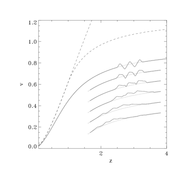
Figure 1: Evolution of a triangular wave train in a shallow wind (the latter shown as dotted line). For clarity, the velocity law is plotted with a negative, vertical offset which increases with time. The dashed lines show the shallow solution with $m=1$ and the critical solution.

Figure 2: Left panel: stable Abbott wave propagation along a shallow velocity law. A sinusoidal perturbation with amplitude $S=0.04$ and period $P=1$ is applied at $z_{\rm e}=2$. Right panel: Abbott wave runaway if the amplitude is doubled to $S=0.08$.

The whole sawtooth pattern moves upstream as an Abbott wave. This is of a prime importance for our understanding of the observed runaway.

Namely, if a perturbation is fed into the wind continuously over time, the whole inner wind is eventually lifted towards larger speeds and mass loss rates. The same is true for the outer wind, first directly by the runaway, and second as a consequence of the accelerated inner gas propagating outwards.

We consider a coherent, sinusoidal velocity perturbation of period $P$ and maximum amplitude $S$, which is fed into the flow at a fixed location $z$. The fundamental hydrodynamic variables used in the code are $\rho$ and $\rho v$. After each time step $\delta t$, perturbations

$$\rho v\rightarrow\rho v+\rho\,\delta v,\qquad\rho\rightarrow\rho(1-\delta v/|A|),$$ (36)

with

$$\delta v=\delta t\,{2\pi S\over P}\cos{2\pi t\over P}$$ (37)

are applied to $\rho v$ and $\rho$ on a single mesh point. The density fluctuations follow from the continuity equation, $\delta\rho/\rho\approx-\delta v/|A|$. For linear waves, the observers frame Abbott speed is $A\approx-1.05$ at $z_{\rm e}=2$ for $m=0.8$.

For sufficiently small amplitudes $S$, $v^{\prime}$ remains positive, and Abbott waves propagate in a stable fashion towards the wind base. This is shown in the left panel of Figure 2, for $P=1$ and $S=0.04$. Doubling the perturbation amplitude to $S=0.08$ implies wind runaway towards the critical solution, as is shown in the right panel of Figure 2. The wind converges to $m=1$ everywhere (not shown). Instead of adopting the critical, accelerating branch, the velocity law jumps at $z>z_{\rm e}$ to the decelerating branch. This is even true for the converged, stationary solution as $t\rightarrow\infty$. (The velocity slope is so mildly negative for $t\rightarrow\infty$ that the wind speed is almost constant above $z_{\rm e}=2$.) We add some further remarks on this issue below.

The runaway results from the occurence of negative velocity gradients. During excitation phases where $v^{\prime}<0$, the resulting line force perturbations are not sufficiently negative to compensate for positive line force perturbations during phases where $v^{\prime}>0$. Net acceleration of the wind results over a full excitation cycle is the consequence.

Figure 3: The runaway time series from Fig. 2, shown with a constant vertical displacement between snapshots. Dashed lines show phases where negative velocity perturbations are applied at $z_{\rm e}$, leading to self-annihilating slopes.

Figure 3 shows again the runaway time series of Fig. 2, with subsequent snapshots displaced vertically for clarity. During the negative perturbation half-cycle, $-\delta v(z_{\rm e})$, negative velocity slopes propagate outwards from below $z_{\rm e}$, and merge with positive slopes propagating inwards from above $z_{\rm e}$. The merging slopes mutually annihilate. After a time $P/2$, the velocity law is left largely unaltered in presence of the perturbation. This causes the dense spacing of curves in Figure 2, especially at $z>z_{\rm e}$, once every perturbation cycle. On this rather flat velocity law, a positive perturbation $+\delta v$ is added during the next half-cycle. Here, inner, positive slopes propagate inwards and separate from outer, negative slopes which propagate outwards. Obviously, runaway is caused by positive perturbations, but its deeper origin is that negative perturbations are self-annihilating, and cannot balance positive ones.

The runaway terminates when $z_{\rm e}$ comes to lie on the critical solution, and Abbott waves can no longer propagate inwards.

The velocity gradient at $z>z_{\rm e}$ is then still negative, and in most of our simulations remains negative at all times: at $z_{\rm e}$, the wind jumps to the decelerating branch with $m=1$, which causes a kink in $v(z)$. Runaway perturbations above $z_{\rm e}$ would be required to establish a critical, accelerating velocity law in the outer wind. For certain combinations of model parameters, we find instead a critical solution with $v^{\prime}>0$ over the whole mesh. The near-plateau above $z_{\rm e}$ evolves then towards larger speeds, and the velocity kink propagates outwards, eventually leaving the mesh. We believe that this is an artefact caused by boundary-induced, numerical runaway (Feldmeier & Shosman 2001). The latter can even occur when non-reflecting Abbott boundary conditions are used, via non-WKB (standing?) waves; our Riemann boundary conditions were formulated to annihilate WKB waves only. We prefer the situation $v^{\prime}<0$ for $z>z_{\rm e}$ over any numerical runaway which would assist the present, physical runaway in reaching the critical solution. A future analysis of outer boundary conditions has to clarify this issue of the outer wind velocity law.

We can still test the stability of the full, critical solution, as is done in Figure 4. Above the critical point, perturbation phases with $v^{\prime}>0$ and $v^{\prime}<0$ combine here, and propagate outwards as a smooth, marginally stable Abbott wave.

Figure 4: The critical, CAK solution is stable with respect to Abbott waves excited above the critical point. Perturbation phases with positive and negative $v^{\prime}$ combine to an outward propagating, harmonic Abbott wave.

3.3 Stationary overloaded winds

So far, we assumed that wind perturbations are located above the critical point. We consider now the opposite case, $z_{\rm e}<z_{\rm c}$.

Figure 5 shows the wind velocity law resulting from a perturbation location $z_{\rm e}=0.8$ on the critical solution. A period $P=0.3$ was chosen. A stationary wind with a broad deceleration region, $v^{\prime}<0$, develops. Abbott waves propagate outwards from $z_{\rm e}$ through the decelerating wind. Since the CAK critical point, which is the bottleneck of the flow, lies in the deceleration regime, the present solution should be overloaded. Indeed, the mass loss rate is found to be $m=1.05$.

Figure 5: Velocity law for a wind with harmonic perturbation at $z_{\rm e}=0.8$, below the critical point $z_{\rm c}=1$. The wind converges to a stationary, overloaded solution. The dotted line shows the initial conditions, the critical CAK solution.

This result is readily understood. The flow at $z_{\rm e}$ is still sub-abbottic, because $z_{\rm e}<z_{\rm c}$. Runaway to larger $v$ occurs until inward propagation from $z_{\rm e}$ becomes impossible. The velocity at $z<z_{\rm e}$ is then everywhere larger than the critical speed. The runaway stops when the inward Abbott speed becomes zero in the observers frame. We are interested in a stationary solution, hence, $A=0$ in (33), implying $mw^{\prime}=g_{\rm c}$. The square root in (10) has to vanish then, hence $m=g_{c}/g$.

So far, we restricted ourselves to $g=g_{c}$ and $m=1$. But critical points can also occur along overloaded solutions. In this case, $m=g_{\rm c}/g(z_{\rm c})>1$, and the square root in (10) becomes imaginary at $z>z_{\rm e}$. Remember that $g_{\rm c}$ refers to gravity at the critical point of the critical solution, which is the maximum of $g$. Hence, $g(z_{\rm c})<g_{\rm c}$ for any other possible critical point. The perturbation site $z_{\rm e}$ stops communicating with the wind base only when it becomes a critical point itself. At $z_{\rm e}$, the overloaded wind jumps to the decelerating branch, resulting in a kink in the velocity law. This kink has all the attributes of a critical point. Especially, as an Abbott wave barrier, it shuts off communication with the wind base.

It is easily seen that a critical point at $z<z_{\rm e}$ would imply that $z_{\rm e}$ is already super-abbottic, which cannot happen during runaway. Since $g(z)$ is a monotonically growing function with a maximum $g_{c}$, the perturbation site $z_{\rm e}<z_{\rm c}$ is the first one that becomes critical to Abbott waves on the evolving overloaded solution. We emphasize that the amount of overloading is solely determined by $z_{\rm e}$.

At some height above the gravity maximum, the decelerating solution jumps back to the accelerating branch, giving a second kink: the wind has overcome the bottleneck, and starts to accelerate again. In the present wind model, the (imaginary, overloaded) solution becomes real again at $z=1/z_{\rm e}$ ($z_{\rm e}$ being the location where the solution becomes first imaginary). For $z_{\rm e}=0.8$, the overloading is $m=1.025$ and the wind can start accelerating again at $z=1.25$. In the simulation however, $m=1.05$, and the second kink occurs at $z=1.6$. The discrepance in $m$ can be attributed to mesh resolution, which blurrs out $z_{\rm e}$. This leaves still unanswered why the wind ‘waits’ so long before it starts accelerating again.

Furthermore, starting with a shallow wind as initial conditions instead of a critical wind, the simulation converges again to an overloaded solution. However, the jump from the decelerating back to the accelerating branch does not terminate on the steep, but already on the shallow overloaded solution with $m=1.05$. This is a numerical artefact caused by non-reflecting, outer boundary conditions, which try to maintain shallow solutions. As above, we prefer this situation over any boundary-induced, numerical runaway.

A third kink may occur. For realistic radiative fluxes above accretion disks, we find that at still larger distances from the disk, the line force drops below absolute gravity for all solution types (Feldmeier & Shlosman 1999). Another jump to the decelerating branch is unavoidable. Since the local wind speed is much larger than the local escape speed, the velocity law stays essentially flat above this kink.

3.4 Time-dependent overloaded winds

Already a minor increase in the mass loss rate causes a broad deceleration region. This is a consequence of $g(z)$ having a broad maximum at $z_{c}$. Integrating $w^{\prime}(z)=vv^{\prime}$ numerically, we find that $v(1/z_{\rm e})=0$ for $z_{\rm e}=0.660$. If $z_{\rm e}$ is still smaller, the gas starts to fall back towards the photosphere before it reaches $1/z_{\rm e}$, and collides with upwards streaming gas. A stationary solution is no longer possible. Figure 6 shows, for $z_{\rm e}=0.5$, that an outward propagating sequence of shocks and dense shells forms. The shock spacing is determined by the perturbation period.

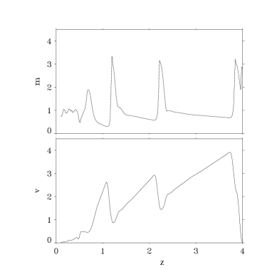
Figure 6: Velocity $v$ and mass flux $m$ of a wind perturbed at $z_{\rm e}=0.5$. During each perturbation cycle, gas falls back towards the photosphere and collides with upwards streaming gas. Shocks form, and propagate outwards.

As a technical comment, we add that the latter simulation tends to develop extremely strong rarefactions and, correspondingly, very large velocities. The latter cause the Courant time step to approach zero. This is a well-known artefact of the power law form of the CAK line force, $g_{\rm l}\propto(v^{\prime}/\rho)^{\alpha}$, implying $g_{\rm l}\rightarrow\infty$ as $\rho\rightarrow 0$. The true line force reaches instead a finite maximum in a flow which is optically thin even in very strong lines (Abbott 1982). This is achieved by truncating the line distribution function (Owocki, Castor, & Rybicki 1988). Using a simpler approach which suffices for the present purposes, we simply truncate $m$ at large values.

Even for $z_{\rm e}=0.660$ implying negative speeds, overloading is small, only 9% above the critical CAK value ($m=1.088$). This shows that the CAK mass loss rate is a significant upper limit for mass loss rates in LDWs, with or without mass overloading. If overloading occurs, it should be detectable only via broad, decelerating flow regions.

It is important to distinguish the present runaway from the well-known line-driven instability (Lucy & Solomon 1970; Owocki & Rybicki 1984; Lucy 1984), which leads to strong shocks and dense, narrow shells in the wind. For perturbations longer than the Sobolev scale, the instability can be understood as a linear process in second-order Sobolev approximation, including curvature terms $v^{\prime\prime}$. By contrast, runaway occurs already in first-order Sobolev approximation, yet, finite perturbations are required to achieve $v^{\prime}<0$.

3.5 Triggering perturbations

Amplitudes. Still, even perturbations with small amplitudes can lead to runaway, if their wavelength is sufficiently short to cause negative $v^{\prime}$. One expects, however, that dissipative processes like heat conduction prevent runaway for short wavelength perturbations.

Coherence. In a hydrodynamic instability, a feedback cycle amplifies small initial perturbations. Even perturbations of short duration trigger unstable growth. By contrast, the present wind runaway requires a continuously maintained perturbation seed. No feedback occurs. The runaway is a pure wave feature caused by the peculiar $v^{\prime}$-asymmetry of the line force.

Perturbations of short duration lead to a localized runaway. The wind is shifted towards larger $v$ and $m$ within a small $z$ interval. If the perturbation ceases, so does the runaway. The region of increased $v$ and $m$ propagates upstream as an Abbott wave, and eventually lifts the wind base to a stable shallow solution with slightly higher $m$. Successive Abbott waves lift the wind until the critical or an overloaded solution is reached.

Surrounding medium. One expects that mismatches at the outer boundary, where the wind propagates into a medium of given properties, create perturbations which can trigger runaway. This is supported by the fact that at large $z$ the velocity law is almost flat, and even small-amplitude perturbations can cause $v^{\prime}<0$. The Abbott speed is large at large $z$, since $A\sim 1/\sqrt{v^{\prime}}$, hence perturbations propagate inwards quickly. We performed tests with the outer boundary at $z=40$. Inherent interpolation errors are sufficient then to set off boundary runaway.

Other sources. Inner wind perturbations could occur due to prevalent shocks from the line driven instability (Owocki et al. 1988). The critical point lies usually close to the sonic point (Owocki & Puls 1999; Feldmeier & Shlosman 1999), and it is therefore not easy to contemplate strong shocks below the critical point. This means that perturbations at large and not at small $z$ dominate the runaway, and drive the wind to a critical solution. Hence, overloaded winds formed by internally-generated perturbations should be rare.

3.6 Critical points and mass loss rate

We discuss here some general issues related to critical points and mass loss rates in different types of stellar winds.

Holzer’s wind laws. The idea that upstream, inwards propagating waves adapt the wind base to outer (boundary) conditions is fundamental to solar wind theory. From this grew the recognition that an outward force which is applied above the sonic (critical) point does not affect the mass loss rate, but only accelerates the flow; whereas a force applied below the sonic point increases the mass loss rate, but has a vanishing effect on terminal wind speeds (Leer & Holzer 1980; Holzer 1987). These ‘wind laws’ have proven to be of interest for cases far beyond the coronal winds for which they were first applied. We refer to Lamers & Cassinelli (1999) for a detailed discussion.

Most relevant to us is the case of a force applied in the subcritical wind region, causing enhanced mass loss. For coronal winds, the subsonic region has essentially a barometric density stratification. Any extra force assisting the pressure gradient helps to establish a larger scale height. From the continuity equation, a shallower velocity gradient results, though the terminal speed is hardly affected. The corresponding situation, analyzed by us for LDWs, is even simpler. No outward force occurs besides line driving. Our choice of zero sound speed emphasizes that the barometric stratification plays no role for mass loss runaway or for establishing an overloaded solution. Overloaded LDW solutions have a steeper velocity gradient than the critical solution, as can be seen from eq. (7). Physically, a steeper velocity gradient is required to create a generalized critical point below the CAK critical point. In LDWs, a critical acceleration $w^{\prime}=vv^{\prime}$, not a critical speed $v$ is adopted at the critical point, and prevents further Abbott wave runaway.

Physical relevance of critical points. The physical relevance of the CAK critical point was questioned by Lucy (1975, 1998), arguing that it may be an artifact of Sobolev approximation. Holzer (1987, p. 296) doubts that critical points, i.e., singularities of the flow equations, generally coincide with those points beyond which “information relevant to the acceleration of the wind” can no longer be transported upstream. We have tried in the present paper to re-establish a more traditional viewpoint (Courant & Friedrichs 1948; Courant & Hilbert 1968), namely that a critical point as a mathematical singularity leaves certain derivatives of flow quantities undetermined. This is only possible along characteristics, which are the space-time trajectories of the specific waves in the problem. This establishes the transonic (or trans-abbottic, etc) nature of the critical point. Similarly, one can argue: the critical point is a singularity because different solution branches cross there. Hence, by passing continuously from one branch to another (actually: by staying on a certain branch), higher-order or weak discontinuities appear in the flow properties; for LDWs, in $v^{\prime\prime}$. Again, weak discontinuities propagate at characteristic wave speed, making the critical point transonic.

Mass loss rate as an eigenvalue. We remind the reader of a deep difference between coronal and line-driven winds. For coronal winds, the mass loss rate is a free parameter within wide margins, and is determined by the base density. For LDWs, on the other hand, the mass loss rate is a unique, discrete eigenvalue (CAK). This is a consequence of the line acceleration depending on $\rho$, see Lamers & Cassinelli (1999).

Abbott speed and speed of light. In the literature, the propagation speed of radiative waves is occasionally identified with the speed of light. This is not true in general: the Abbott speed and, in magnetized flows, the Alfvén speed are smaller than the speed of light. To make the point totally obvious, note that the diffusion speed of photons through stellar interiors is much smaller than the speed of light. The basic cause is here the same as for Abbott waves: optical depths larger than unity.

3.7 Deep-seated X-rays, infall, and mass-over-loading

Besides adapting the wind base to outer flow conditions, we find that Abbott waves can even lead to mass inflow. This seems like a novel feature of these waves and it leads to interesting observational consequences, like explaining the formation of hard X-rays anomalously close to the surfaces of hot stars. Formation depths of $r\approx 1.1\,R_{\ast}$ are deduced from X-ray emission lines observed with the Chandra satellite (for $\zeta$ Ori: Waldron & Cassinelli 2000; for $\zeta$ Pup: Cassinelli et al. 2001). The favored model for X-ray emission from hot stars is via strong shocks (Lucy 1982) from the de-shadowing instability (Lucy & Solomon 1970; Owocki & Rybicki 1984). The shocks become strongest in collisions of fast clouds with dense gas shells (Feldmeier, Puls, & Pauldrach 1997). From theoretical arguments (line drag effect: Lucy 1984) and numerical simulations it appears that this shock scenario cannot explain X-rays originating from the small heights mentioned above.

Howk et al. (2000) suggest gas infall as possible origin of X-rays from near the photosphere. They consider a ballistic model of stalled wind clouds falling back towards the star, to explain the hard X-rays observed from $\tau$ Sco (Cassinelli et al. 1994). At any instant, $\approx 10\%$ of the mass flux from the star resides in numerous, $\geq 1000$, clouds which barely reach distances of $r=2\,R_{\ast}$ before falling back inwards. The overall resemblance of this cloud model with time-dependent wind overloading as shown in Fig. 6 is striking. In the latter case, the overloading is sufficiently mild that upstreaming gas can push downfalling clumps outwards (cf. the drag force of ambient wind gas in Howk et al.). Stronger overloading is achieved by shifting the Abbott wave source further inwards, but cannot be addressed using our simple numerical approach. Clearly, two-dimensional simulations are required to model true infall. A systematic study relating the Howk et al. approach with ours is in preparation.

Note that the critical point in stellar wind models accounting for the finite cone effect lies at $r\leq 1.1\,R_{\ast}$ (Pauldrach et al. 1986). An overloaded wind starts to decelerate below the critical point, and may already reach negative or infall speeds at similarly small heights. This shows the relevance of overloading in understanding the Chandra observations mentioned above. The topic of stalling and backfalling gas has aquired some general attention in recent papers on LDWs, and is discussed in different contexts by Friend & Abbott (1986), Poe et al. (1990), Koninx (1992), Proga, Stone, & Drew (1998), and Porter & Skouza (1999).

We finally mention another idea related to overloaded flows, which has played some role in sharpening our understanding of coronal winds. Cannon & Thomas (1977) and Thomas (1982) challenged Parker’s (1958, 1960) theory of the solar wind. They postulated an outwards directed, sub-photospheric mass flux. In analogy with a Laval nozzle (e.g., Chapman 2000, Chapter 7) into which a too strong mass or energy influx is fed (Cannon & Thomas 1977 use the terminology ‘imperfect nozzle’ instead of ‘overloading’), the solar outflow should choke, creating shocks below the nozzle throat, or the critical point of the smooth (perfect nozzle) flow. The shocks are responsible for heating the chromosphere and corona, making the latter a consequence, not the origin of outflow from Sun. This model was ruled out by Parker (1981) and Wolfson & Holzer (1982).

Still, it leads over to another interesting difference between coronal and Laval nozzle flows on the one side and LDWs on the other: the former two do not allow for continuous, overloaded solutions; instead, overloaded flows have shocks in the $vr$ plane where the critical point resides. By contrast, overloaded LDWs show jumps in the critical $vv^{\prime}$-$r$ plane, i.e., jumps in the wind acceleration which correspond to kinks in a continuous velocity law.

4 Summary

We have studied the stability of shallow and steep solutions for accretion disk and stellar line driven winds. This was done by introducing flow perturbations into the wind at a fixed height. For sufficiently large perturbation amplitudes, negative velocity gradients occur in the wind and cause runaway towards the critical solution. The origin of this runaway is an asymmetry in the line force: negative velocity gradients cause a force decrease which cannot balance the force increase during phases where the velocity law gets steepened. Net acceleration results over a full perturbation cycle.

A new type of waves, termed Abbott waves, are exited by the perturbations. They provide a communication channel between different parts of the wind and define an additional critical point in the flow, downstream from the sonic point. Shallow solutions are subcritical everywhere, steep solutions are supercritical. Along shallow solutions, Abbott waves propagate upstream towards the photosphere at a high speed as a radiative mode, and creep downstream at a fraction of the sonic speed as an acoustic mode. The critical solution is the one that switches continuously from the shallow to the steep branch at the critical point.

Inward propagating Abbott waves turn the local, asymmetric response to velocity perturbations into a global runaway towards the critical solution. The converged, steady wind solution depends on the location of seed perturbations. Three spatial domains can be distinguished. (i) If perturbations are prevalent in outer wind regions, above the critical point, the wind settles on the critical solution. (ii) If perturbations occur just below the critical point, runaway proceeds to a stationary, so-called overloaded solution. Such a flow is characterized by a broad deceleration domain. The line force cannot balance gravity in a vicinity of the critical point (the bottleneck of the flow) because of a supercritical mass loss rate. (iii) Perturbations close to the photosphere result in the wind being decelerated to negative speeds. Gas falls back towards the photosphere, and collides with upwards streaming gas. A time-dependent, overloaded wind results with a train of shocks and shells propagating outwards.

The runaway mechanism discussed here depends solely on the asymmetry of the line force with respect to velocity perturbations which cause local flow deceleration, $dv/dr<0$. It should, therefore, be a robust feature and not depend on Sobolev approximation.

- [1]
- [2] Abbott, D.C. 1980, ApJ, 242, 1183
- [3] Abbott, D.C. 1982, ApJ, 259, 282
- [4] Cannon, C.J. & Thomas, R.N. 1977, ApJ, 211, 910
- [5] Cassinelli, J.P., Cohen, D.H., MacFarlane, J.J., Sanders, W.T. & Welsh, B.Y. 1994, ApJ, 421, 705
- [6] Cassinelli, J.P., Miller, N.A., Waldron, W.L., MacFarlane, J.J. & Cohen, D.H. 2001, ApJ, 554, L55
- [7] Castor, J.I., Abbott, D.C. & Klein, R.I. 1975, ApJ, 195, 157 (CAK)
- [8] Chapman, C.J. 2000, High Speed Flow (Cambridge: Cambridge Univ. Press)
- [9] Courant, R. & Friedrichs, K.O. 1948, Supersonic Flow and Shock Waves (New York: Interscience Publishers)
- [10] Courant, R. & Hilbert, D. 1968, Methoden der Mathematischen Physik (Berlin: Springer)
- [11] Feldmeier, A., Puls, J. & Pauldrach, A. 1997, A&A, 322, 878
- [12] Feldmeier, A. & Shlosman, I. 1999, ApJ, 526, 344
- [13] Feldmeier, A. & Shlosman, I. 2000, ApJ, 532, L125
- [14] Feldmeier, A., Shlosman, I. & Hamann, W.-R. 2001, ApJ, submitted
- [15] Friend, D.B. & Abbott, D.C. 1986, ApJ, 311, 701
- [16] Holzer, T.E. 1987, IAU Symp. #122, Circumstellar Matter (Dordrecht: Reidel), 289
- [17] Howk, J.C., Cassinelli, J.P., Bjorkman, J.E. & Lamers, H.J.G.L.M. 2000, ApJ, 534, 348
- [18] Koninx, J.-P. 1992, Ph. D. thesis, Utrecht Univ.
- [19] Lamb, H. 1932, Hydrodynamics (New York: Dover)
- [20] Lamers, H.J.G.L.M. & Cassinelli, J.P. 1999, Introduction to Stellar Winds (Cambridge: Cambridge Univ. Press)
- [21] Leer, E. & Holzer, T.E. 1980, JGR, 85, 4681
- [22] Lucy, L.B. 1975, Memoires Societe Royale des Sciences de Liege, 8, 359
- [23] Lucy, L.B. 1982, ApJ, 255, 286
- [24] Lucy, L.B. 1984, ApJ, 284, 351
- [25] Lucy, L.B. 1998, in Cyclical Variability in Stellar Winds, ed. L. Kaper & A.W. Fullerton (Berlin: Springer), 16
- [26] Lucy, L.B. & Solomon, P.M. 1970, ApJ, 159, 879
- [27] Owocki, S.P. & Rybicki, G.B. 1984, ApJ, 284, 337
- [28] Owocki, S.P. & Rybicki, G.B. 1986, ApJ, 309, 127
- [29] Owocki, S.P., Castor, J.I. & Rybicki, G.B. 1988, ApJ, 335, 914
- [30] Owocki, S.P. & Puls, J. 1999, ApJ, 510, 355
- [31] Parker, E.N. 1958, ApJ, 128, 644
- [32] Parker, E.N. 1960, ApJ, 132, 175
- [33] Parker, E.N. 1981, ApJ, 251, 266
- [34] Pauldrach, A., Puls, J. & Kudritzki, R.P. 1986, A&A, 164, 86
- [35] Poe, C.H., Owocki, S.P. & Castor, J.I. 1990, ApJ, 358, 199
- [36] Porter, J.M. & Skouza, B.A. 1999, A&A, 344, 205
- [37] Proga, D., Stone, J.M. & Drew, J.E. 1998, MNRAS, 295, 595
- [38] Rybicki, G.B. & Hummer, D.G. 1978, ApJ, 219, 654
- [39] Thomas, R.N. 1982, ApJ, 263, 870
- [40] Waldron, W.L. & Cassinelli, J.P. 2000, ApJ, 548, L45
- [41] Wolfson C.J. & Holzer, T.E. 1982, ApJ, 255, 610