Detecting Clusters of Galaxies in the Sloan Digital Sky Survey I : Monte Carlo Comparison of Cluster Detection Algorithms

Abstract

We present a comparison of three cluster finding algorithms from imaging data using Monte Carlo simulations of clusters embedded in a 25 $\mbox{deg}^{2}$ region of Sloan Digital Sky Survey (SDSS) imaging data: the Matched Filter (MF; Postman et al. 1996), the Adaptive Matched Filter (AMF; Kepner et al. 1999) and a color-magnitude filtered Voronoi Tessellation Technique (VTT). Among the two matched filters, we find that the MF is more efficient in detecting faint clusters, whereas the AMF evaluates the redshifts and richnesses more accurately, therefore suggesting a hybrid method (HMF) that combines the two. The HMF outperforms the VTT when using a background that is uniform, but it is more sensitive to the presence of a non-uniform galaxy background than is the VTT; this is due to the assumption of a uniform background in the HMF model. We thus find that for the detection thresholds we determine to be appropriate for the SDSS data, the performance of both algorithms are similar; we present the selection function for each method evaluated with these thresholds as a function of redshift and richness. For simulated clusters generated with a Schechter luminosity function ($M_{r}^{*}=-21.5$ and $\alpha=-1.1$) both algorithms are complete for Abell richness $\;\buildrel>\over{\sim}\;$ 1 clusters up to $z\sim 0.4$ for a sample magnitude limited to $r=21$. While the cluster parameter evaluation shows a mild correlation with the local background density, the detection efficiency is not significantly affected by the background fluctuations, unlike previous shallower surveys.

1 Introduction

Over the past few decades, clusters of galaxies have been used as valuable tools for cosmological studies: they are tracers of large scale structure (Bahcall 1988, Huchra et al. 1990, Nichol et al. 1992, Nichol et al. 1994, Peacock & Dodds 1994, Collins et al. 2000), their number density is a constraint on cosmological models (Gunn & Oke 1975, Hoessel, Gunn & Thuan 1980, Evrard 1989, Bahcall et al. 1997, Carlberg et al. 1997, Oukbir & Blanchard 1997, Reichart et al. 1999), and they act as laboratories for probing the formation and evolution of galaxies and their morphologies (Dressler 1980, Butcher & Oemler 1984, Gunn & Dressler 1988, Dressler et al. 1997). While it is sometimes sufficient simply to have a large sample of clusters, most cosmological studies require a homogeneous sample with accurate understanding of the selection biases and the completeness of the catalog.

The Abell cluster catalog is by far the most widely used catalog to date (Abell 1958; Abell et al. 1989, hereafter ACO). Like some of the other cluster catalogs that are available (e.g., Zwicky et al. 1968; Gunn et al. 1986), the Abell catalog was constructed entirely by visual inspection of photographic plates. Although the human eye is a sophisticated and efficient detector for galaxy clusters, it suffers from subjectivity and incompleteness, and visual inspection is extremely time consuming. For cosmological studies, the major disadvantage of such visually constructed catalogs is that it is difficult to quantify selection biases and the selection function.

The main motivation for automated cluster finding schemes is thus to overcome these major drawbacks of visual catalogs, namely speed, objectivity and reproducibility. The first automated cluster finding in optical surveys was attempted by Shectman (1985), and was followed by several variants of this peak finding method; Lumsden et al. (1992) with the EDSGC (Nichol, Collins, & Lumsden 2001) and Dalton et al. (1992) with the APM survey (Maddox et al. 1990). Lahav & Gull (1989) introduced the concept of fitting the observed apparent diameter distribution to the absolute distribution to obtain an estimate of the distance to each cluster, which led to the development of the Matched Filter Algorithm (Postman et al. 1996, hereafter P96). The matched filter technique has been widely used, and several variants have been further developed (Kawasaki et al. 1998; Schuecker & Böhringer 1998; Lobo et al. 2000), including the Adaptive Matched Filter (Kepner et al. 1999; hereafter K99, Kepner & Kim 2000). In addition, thanks to the availability of multi-band CCD imaging data, several cluster finding methods have been put forward that utilize the color characteristics of galaxy clusters (Annis et al. 2001, Gladders & Yee 2000, Goto et al. 2001, Nichol et al. 2000b). While these methods can be efficient, each inevitably has its own biases, depending on the nature and extent of constraints that have been imposed for the selection. Little effort has been made to date to compare the performances of these different methods.

In this paper, we present a comparison of three different cluster finding algorithms, using a Monte Carlo experiment with simulated clusters. The algorithms we analyze are the Matched Filter algorithm (P96), the Adaptive Matched Filter algorithm (K99), and the Voronoi Tessellation Technique, which is introduced in detail in §2.2. The last technique, which uses color information, is in part based on previous cluster finding efforts that use the classical Voronoi Tessellation as a peak finder (Ramella et al. 1998, Ebeling 1993, Kim et al. 2000), but is introduced here for the first time in its current form. These three methods constitute the basis of a cluster catalog derived from 150 $\mbox{deg}^{2}$ of Sloan Digital Sky Survey (York et al. 2000; hereafter SDSS) commissioning data, which we present in Paper II (Kim et al. 2001). Work in progress (Bahcall et al. 2001) will present cluster catalogs using a wide range of finding techniques. This paper is thus geared towards understanding the behaviour of the cluster finding algorithms in the SDSS data.

In §2 we describe the various cluster detection algorithms, and in §3 we present the Monte Carlo experiment in which these cluster finding algorithms were run. The results and comparison between methods are presented in §4. We summarize in §5. Throughout this paper we assume a cosmology in which $\Omega_{m}=0.3$, $\Omega_{\Lambda}=0.7$ and $H_{0}=70\mbox{km}\,\mbox{s}^{-1}\,\mbox{Mpc}^{-1}$ unless noted otherwise.

2 Cluster Selection Algorithms

The Matched Filter algorithm, which was first presented as a fully automated cluster finding scheme in P96, has been widely adapted for a variety of cluster detection efforts (e.g., Olsen et al. 1999, Scodeggio et al. 1999, Bramel et al. 2000; hereafter BNP00, Postman et al. 2001, Willick et al. 2001). The Adaptive Matched Filter algorithm (K99, Kepner & Kim 2000), which is described below, should be a substantial improvement both in content and efficiency over the original Matched Filter algorithm; the major changes being the adoption of a full likelihood function and the incorporation of 3-D (redshift) information. Nevertheless, unlike the P96 Matched Filter, the Adaptive Matched Filter algorithm has not yet been applied to real data, and therefore lacks the optimizations and adaptations that exposure to real data would give. Thus we have chosen to apply both the original Matched Filter (hereafter MF) and the Adaptive Matched Filter (hereafter AMF) for comparison and cross-checking purposes. Although the AMF should in theory converge to the MF results in the 2-D case, there are various differences in the details of the two codes (e.g., peak selection criteria, final parameter evaluations, likelihood function detailed further below) that can cause the final results to differ somewhat. The fact that they are two completely independent codes written in two different languages (C and IDL) also makes the cross check particularly useful.

The Matched Filter technique is an efficient likelihood method for finding clusters in two dimensional imaging data. A model cluster radial profile and galaxy luminosity function are used to construct a matched filter in position and magnitude space from which a cluster likelihood map is generated. Using the magnitudes rather than simply searching for density enhancements suppresses false detections that occur by chance projection. Of course, the results are dependent on the assumed filter shape and extent; they are thus affected by the assumptions made for the universal radial profile and cluster luminosity function used in the algorithm. In other words, the cluster parameters that are derived from the algorithm are somewhat dependent on the model that was assumed for the cluster, and the probability for detecting a certain cluster may differ as the cluster shape varies (e.g., spherical vs. elongated), or as the cluster parameters deviate from the assumed cluster model. In fact most clusters are elongated, and are known to have a variety of shapes (e.g., Bautz-Morgan (1970) type, Rood-Sastry (1971) type). The third method, the Voronoi Tessellation Technique (hereafter VTT), was in part motivated by this model-dependent aspect of the Matched Filter algorithms (MF and AMF), to examine if any severe biases occur in the selection due to model assumptions. In addition to the fact that the VTT assumes no intrinsic cluster properties (except for very mild constraints in color-magnitude space, see below), it is simple and fast (for $n=10^{6}$ galaxies, it takes seconds on a 400 MHz CPU to evaluate Voronoi Tessellation).

The details of the MF and the AMF are given in the respective references, so here we only describe them briefly (§2.1), mainly comparing them carefully and emphasizing their differences. This is followed by a detailed recipe for the VTT in §2.2.

2.1 The Matched Filter Techniques

The foundation for both matched filter techniques is the model for the total number of galaxies per unit area per unit observed flux $l$:

$$n_{\mbox{model}}(\theta,l,z_{c})\,dA\,dl=[n_{f}(l)+\Lambda_{cl}n_{c}(\theta,l,z_{c})]\,dA\,dl,$$ (1)

which consists of contributions from background field galaxies ($n_{f}$) and the cluster galaxies ($\Lambda_{cl}n_{c}$) at redshift $z_{c}$, where $\Lambda_{cl}$ is the cluster richness measure (see below). Here, $\theta$ is the angular distance from the cluster center, and $dA=2\pi\theta\,d\theta$. The background number density ($n_{f}$) is simply taken from the global number counts of the survey. The essential ingredient of the matched filter is the model for the cluster number density, $\Lambda_{cl}n_{c}$, which is a product of a projected cluster density profile and a luminosity profile for a cluster at redshift $z_{c}$:

$$\Lambda_{cl}n_{c}(\theta,l;z_{c})=\Lambda_{cl}\Sigma_{c}(r)\left({dr\over d\theta}\right)^{2}\phi_{c}(L)\left({dL\over dl}\right),$$ (2)

where $r$ is the projected comoving radius and $L$ is the absolute luminosity. The conversion from physical units to apparent units includes proper treatment for cosmology and the K-correction. For the projected density profile we use the modified Plummer law model (see K99 Appendix A),

$$\Sigma_{c}(r)\propto\left\{\begin{array}[]{l}[1+(r/r_{c})^{2}]^{-n/2}-[1+(r_{\mbox{max}}/r_{c})^{2}]^{-n/2}\ \ \ \ \mbox{for}\ (r<r_{\mbox{max}})\\ 0\ \ \ \ \mbox{for}\ (r\geq r_{\mbox{max}})\end{array}\right.$$ (3)

where $n\approx 2$, the slope of the profile, $r_{c}$ is the core radius and $r_{\mbox{max}}$ is a cutoff radius which approximates the extent of a cluster. This cutoff radius naturally constrains the radius of the search; forcing $\Sigma_{c}(r_{\mbox{max}})=0$ is equivalent to putting a “taper” on the filter which reduces the “sidelobes” and narrows the “beam”. This is standard practice in detection theory, which improves the spatial accuracy and makes the process more robust (at the cost of slightly reducing the sensitivity of the filter), as well as reducing the contamination that arises from other nearby clusters.

Any method of smoothing the data consists of choosing a filter shape and a filter bandwidth. Numerical experiments show that the efficiency of the estimator is much more sensitive to the filter bandwidth than is the filter shape itself (Silverman 1986). Hence determining the appropriate values of $r_{\mbox{max}}$ and $r_{c}$ is more important than our particular choice of the cluster profile functional form. P96 (see §4 in their paper) discuss the effect that the cutoff radius has on their detection efficiency and conclude $r_{\mbox{max}}=1$$h^{-1}$ Mpc as an optimal choice, which we adopt as an appropriate value. Increasing the value of $r_{\mbox{max}}$ further will significantly degrade the signal-to-noise ratio; the cluster signal will go down since less weight is given to the core, and noise from the background and nearby clusters will increase as more weight is given to galaxies at larger radii.

For the luminosity profile we adopt a standard Schechter luminosity function (Schechter 1976),

$$\phi_{c}(L)dL\propto(L/L^{*})^{\alpha}e^{-L/L^{*}}d(L/L^{*}).$$ (4)

The overall normalizations of $\Sigma_{c}$ and $\phi_{c}$ are chosen such that the cluster richness measure $\Lambda_{cl}$ is the total cluster luminosity within $r_{\mbox{max}}$ in units of $L^{*}$, i.e., $L_{cl}(\leq r_{\mbox{max}})=\Lambda_{cl}L^{*}$ (see P96 and K99 for details). The Abell richness $N_{A}$ is defined by the number of cluster galaxies (within $r<1.5$$h^{-1}$ Mpc) with magnitudes between $m_{3}$ and $m_{3}+2$, where $m_{3}$ is the magnitude of the third brightest galaxy in the cluster. The Abell Richness Class (RC; Abell 1958) is determined by this quantity $N_{A}$; $30\leq N_{A}\leq 49$ for RC = 0, $50\leq N_{A}\leq 79$ for RC = 1, $80\leq N_{A}\leq 129$ for RC = 2, and $130\leq N_{A}\leq 199$ for RC = 3. The relation between $N_{A}$ and $\Lambda_{cl}$ (with $r_{max}=1$$h^{-1}$ Mpc) is found to be approximately $N_{A}\sim(2/3)\Lambda_{cl}$ (Bahcall & Cen 1993, P96) but with large scatter (P96). This relation is addressed further in Paper II with the clusters detected from the Sloan Digital Sky Survey imaging data.

The difference between the MF and the AMF starts from the definition of the likelihood function. The MF adopts a Gaussian likelihood function, which is based on the assumption that there are enough galaxies in each virtual bin ($j$) in (position, magnitude) space that the Poisson probability distribution can be approximated by a Gaussian. Furthermore, it assumes that the background galaxy distribution ($n_{f}$) is uniform and large enough to dominate the noise, therefore the likelihood can be written as,

$${\cal L}(\theta)=\sum_{j}-2\ln P_{j}=-2\sum_{j}\ln\left[{1\over\sqrt{2\pi n_{f}^{(j)}}}\exp\left(-{(n^{(j)}_{\mbox{data}}-n^{(j)}_{\mbox{model}}(\theta))^{2}\over 2n_{f}^{(j)}}\right)\right].$$ (5)

By approximating the summation with an integral, using Eq. (1) for $n_{\mbox{model}}$, setting $\delta\equiv n_{c}/n_{f}$, and dropping all terms irrelevant to $\theta$, one obtains a likelihood function that is linear in the data and easy to calculate:

$${\cal L}=\Lambda_{cl}\sum_{i}\delta_{i},\ \ \ \ \mbox{where}\ \ \ \Lambda_{cl}={\sum_{i}\delta_{i}\over\int\delta(\theta,l)n_{c}(\theta,l)dAdl},$$ (6)

where $i$ stands for each galaxy, and the sum is over every galaxy within $r_{\mbox{max}}$. The richness measure $\Lambda_{cl}$ is obtained by first solving the equation $\partial{\cal L}/\partial\Lambda_{cl}=0$ (see K99 Appendix C or P96 for details).

In the AMF, this likelihood function is referred to as the “coarse filter”. Since it is simple and easy to calculate, AMF uses Eq. (6) to construct a “coarse” likelihood map in order to select clusters, by identifying peaks from this map. However, the Gaussian approximation breaks down when there are not enough galaxies, i.e., especially for poor clusters or those at high redshift, and in general the parameters that are evaluated by this “coarse filter” are found to be somewhat biased (P96 discuss empirical correction factors for this bias, which we will not discuss here in detail). Hence, the AMF defines a second likelihood function that assumes a Poisson likelihood instead of a Gaussian (Dalton et al. 1994). This is called the “fine filter” and reduces to:

$${\cal L}_{\mbox{fine}}=-\Lambda_{cl}N_{c}+\sum_{i}\ln(1+\Lambda_{cl}\delta_{i}),$$ (7)

where $\Lambda_{cl}$ is obtained by solving

$$N_{c}=\sum_{i}{\delta_{i}\over 1+\Lambda_{cl}\delta_{i}}.$$ (8)

$N_{c}$ is the number of galaxies expected in a $\Lambda_{cl}=1$ cluster (see K99 Appendix C for the derivation). The resulting fine filter likelihood function is nonlinear and requires more computations to evaluate. However, as it is based on correct statistics, the evaluated cluster parameters (redshift and richness) are expected to be more accurate. The AMF thus adopts a two-layered approach, first to identify clusters by peaks in the coarse filter likelihood map, and then to evaluate proper parameters by the fine filter on those selected cluster positions. The computing time difference between the coarse and the fine filter is due to solving Eq. (8), which must be done at every grid position; using only the fine filter would take approximately 10 times longer. In addition, the AMF approach allows an internal cross check for the evaluation of $z$ and $\Lambda_{cl}$.

The MF and AMF have further differences that turn out, as we will see, to be quite important. The MF uses a uniform grid in 2D space on which the likelihood function is evaluated for a series of redshift values that span the desired redshift range for the cluster search. The grid size is a function of redshift assumed; we use a grid size of 1/2 the core radius at each redshift to ensure proper sampling. Hence the result is a series of likelihood maps evaluated for each assumed redshift, i.e., a map indicating the likelihood for the existence of a cluster at that redshift. The AMF instead uses a so-called “naturally adaptive grid”, evaluating the likelihood function at the galaxy positions themselves, meaning that as we go to higher redshift, the effective resolution becomes finer as necessary. Such a non-uniform grid is slightly more complicated to handle, but ensures that a unique galaxy lies at the center of each cluster, and no computation is wasted on unnecessary positions. As a result, instead of producing series of likelihood maps to be stored at each assumed redshift value, the AMF calculates the likelihood values on a redshift grid for each galaxy separately, and records the redshift and likelihood at which the likelihood is maximized. In other words, the outcome is two quantities at each galaxy: the peak likelihood that a cluster lies at this point, and the corresponding estimated redshift. This saves a significant amount of disk space relative to the MF, and is cleverly structured to reduce an intermediate step in the analysis (step 5 in Table 1), but as we shall see below, this approach has drawbacks.

Once the coarse likelihood map is generated, the two algorithms differ in the final steps of the cluster selection process. The MF, having stored likelihood maps for each redshift bin, finds local maxima in each map, and registers them as candidate clusters when they lie above a prescribed threshold for each map (e.g., 95 percentile within the map; approximately $2\sigma$ level). This is repeated for every redshift bin, then all the cluster candidates from all redshift bins are combined together to filter out overlaps and to find the most likely redshift for each cluster – the redshift where the peak signal is maximized. Each cluster also has a significance of detection $\sigma_{\mbox{det}}$ which is translated from the pixel distribution of the likelihood signals at the final redshift assuming Gaussian statistics. We perform a final cut on this quantity ($\sigma_{\mbox{det}}\geq\sigma_{\mbox{cut}}$), to select significant detections. On the other hand, the AMF has already stored the most likely redshift of each galaxy point, and therefore simply locates the position of the highest likelihood signal, registers it as a cluster, eliminates all galaxies around this point within a sphere of a given cluster size ($r_{\mbox{max}}$), and then looks for the next highest peak, and so on until the likelihood signal (${\cal L}_{\mbox{coarse}}$) drops below a prescribed threshold (${\cal L}_{\mbox{cut}}$). The difference between the two algorithms is not merely the order in which the procedures are executed (the MF locates clusters in angular space first and then determines the redshift, while the AMF determines the redshift first for every point in space and then filters out the clusters in angular space), but that the AMF uses a threshold in likelihood that is constant, thus redshift independent, while the MF uses a threshold that differs for each redshift. The effect that is caused by these differences is discussed in §5.

Finally, the AMF is completed by evaluating the fine filter on the cluster positions that have been selected, then determining the redshift at which the peak of the fine likelihood occurred, and calculating the richness $\Lambda_{cl}$ for that redshift. Table 1 summarizes the procedures and the parameters outlined above for the two Matched Filter algorithms.

2.2 The Voronoi Tessellation Technique

The Voronoi Tessellation made its debut in astrophysics as a convenient way of modeling the large-scale structure of the universe (Icke & van de Weygaert 1987, Ling 1987). With a distribution of seeds (nuclei), Voronoi Tessellation creates polyhedral cells that contain one seed each, enclosing all the volume that is closest to its seed. This is the definition of a Voronoi cell. This natural partitioning of space by Voronoi Tessellation has been used to model the large scale distribution of galaxies. This is achieved by envisioning the seeds to be the expansion centers of “voids”, the planes that intersect two adjacent cells as “walls”, the ridges where three walls intersect as “filaments”, and the vertices where four filaments come together as galaxy clusters (van de Weygaert & Icke 1989).

A slightly different application of the Voronoi Tessellation is to identify X-ray sources by locating the overdensity in X-ray photon counts (Ebeling 1993, Ebeling & Wiedenmann 1993); this is directly related to our application for cluster finding, as we now describe. The galaxy positions are input as the seeds for the Voronoi Tessellation, and the Voronoi cell around each galaxy is interpreted as the effective area that each galaxy occupies in space. Taking the inverse of these areas gives a local density at each galaxy in two dimensions. This information is then used to threshold and select galaxy members that live in highly over-dense regions, which we identify as clusters. We do so by calculating the density contrast at each galaxy position $\delta\equiv(\rho-\bar{\rho})/\bar{\rho}=(\bar{A}-A)/A$, where $A$ is the area of the Voronoi cells, and $\bar{A}$ is the mean area of all cells. We then impose a cut in the density contrast $\delta>\delta_{c}$ to select galaxies in high density environments. One can, in fact, use a more rigorous statistical approach for the detection criteria, using statistics of Voronoi Tessellation for a random distribution of seeds (Kiang 1966; see Ramella et al. 1999, 2001 for details). However, as our approach described below is empirical, we adhere to a simple cut in constant density contrast whose value is tested by a Monte Carlo method using simulated clusters, as described in section 3.3.

The SDSS is currently working on determining photometric redshifts for galaxies in the imaging data, but until they are available, we are confined to working with the two dimensional projected distribution; therefore we need to divide the galaxy sample to group them into comparable redshifts in order to enhance the cluster detectability. Therefore, our recipe for the Voronoi Tessellation Technique utilizes a priori knowledge of characteristics of cluster member galaxies, namely, the color-magnitude relation.

Galaxies within a cluster usually exhibit a tight correlation between their colors and magnitudes. It is well known that the core of a typical rich cluster consists mainly of early type galaxies (i.e., Hubble Types E and S0; Hubble 1936, Oemler 1974, Postman & Geller 1984, Dressler 1980, 1984) which all have very similar red colors. This includes the Brightest Cluster Galaxy (hereafter BCG), whose properties have been well studied (Schneider, Gunn & Hoessel 1983, Postman & Lauer 1995). Figures 1a and b show the color-magnitude relation (C-M diagram) of Abell Clusters 168 and 295 respectively, observed with the SDSS camera; the diagram shows only those galaxies whose cluster membership has been confirmed spectroscopically by the ENACS survey (Katgert et al. 1998). The BCG is marked with a cross, and the narrow horizontal line of galaxies at nearly constant color is referred to as the E/S0 ridgeline (Visvanathan & Sandage 1977, Annis et al. 1999). The color-magnitude relation for E/S0 galaxies has been well known since Baum (1959), who first noted that fainter early type galaxies tend to be bluer, showing a negative slope of the E/S0 ridgeline in C-M diagrams (see also Visvanathan & Sandage 1977, Lugger 1984, Metcalfe et al. 1994). It has been suggested that this slope evolves with redshift (Gladders et al. 1998) and even differs with richness (Stoughton et al. 1998). However, as we see in the C-M diagrams, the slope is very shallow in $(g^{*}-r^{*})$ vs. $r^{*}$ space, and is a negligible effect for the recipe that we now describe.

We will use this characteristic shape in the C-M diagram to select against foreground and background galaxies. Thus we carry out the following approach: first select a redshift, then apply a Voronoi Tessellation on all galaxies in a restricted region of the C-M diagram. This region is shown as solid lines in Figures 1a and b, for a redshift of $z=0.045$, whose limits enclose most of the galaxies that are confirmed members of the cluster. Figures 1c and d show similar C-M diagrams of cluster candidates at higher redshifts, found by both the MF and the AMF from the SDSS. These clusters were visually confirmed with SDSS images, and the redshifts of their BCGs were obtained by the SDSS spectroscopic survey (York et al. 2000). Since membership information is not available, we simply plot all the galaxies that are within 1$h^{-1}$ Mpc radius from the cluster center as circles. For comparison, the C-M distribution of all the galaxies in a survey region of 25 $\mbox{deg}^{2}$ is shown in contours and small dots. The difference in these distributions illustrates the efficiency of using C-M information in discriminating cluster members against the background population. Here again, the areas enclosed by the solid lines are those that are selected for detecting a cluster at $z=0.22$ and $0.35$ respectively, which includes most of the galaxies within $r=1$$h^{-1}$ Mpc around the cluster center.

The empirical C-M limits we use are as follows:

$$r^{*}_{bcg}-1< r^{*} <r^{*}_{bcg}+5$$ (9)

$$ar^{*}+b< (g^{*}-r^{*}) <(g^{*}-r^{*})_{bcg}+0.3$$ (10)

where $a$ and $b$ are given by a simple linear relation with redshift,

$$a=-1.295z-0.084,\ \ \ \ b=30.13z+0.88$$ (11)

where $r^{*}_{bcg}$ and $(g^{*}-r^{*})_{bcg}$ are the Petrosian $r^{*}$ magnitude and the model $g^{*}-r^{*}$ color of the BCG, respectively (see §3.1 for description of magnitudes and colors). These relations are established empirically, by examining the C-M relations of known clusters (e.g., Fig. 1 a,b) and rich clusters of galaxies found by the Matched Filter algorithms and the MaxBCG technique (Annis et al. 2001) from the SDSS data itself. The limits are chosen to generously include most of the galaxies within 1$h^{-1}$ Mpc of the cluster center. The lower limit in magnitude, 5 magnitudes fainter than that of the BCG, is chosen to cover the magnitude range of spectroscopically confirmed cluster members from the ENACS (Katgert et al. 1998) for low redshift clusters ($z<0.1$). This is a moderate coverage of cluster galaxies for a typical cluster luminosity function (corresponding to $M_{lim}\sim L^{*}+3$); also note the recent findings of fossil groups whose difference between the BCG and the second luminous galaxy can be as large as 4-5 magnitudes (Zabludoff & Mulchaey 1998).

These C-M limits are shown in summary for a range of redshifts, from $z=0.04$ to $z=0.5$, in Figure 2. Here, the track of BCGs for the above redshifts are also shown as large dots (filled and open), which provides the basis for determining these limits for each redshift (Eqs. (9) and (11)). Finally, the C-M distribution of all galaxies in the survey region are shown as contours and small dots for comparison. The BCG track is computed assuming a constant absolute magnitude $M(r^{*})_{bcg}=-23$ with no evolution (see Eisenstein et al. 2001). We use the PEGASE evolutionary synthesis model (Fioc & Rocca-Volmerange 1997) to generate the spectral energy distribution of the BCG; this is then redshifted and convolved with the SDSS filter responses to obtain color K-corrections.

Once we have applied these cuts for a given redshift, we apply the Voronoi Tessellation on the resulting distribution of galaxies. We then select all galaxies that satisfy $\delta>\delta_{c}$, where $\delta_{c}$ is a constant overdensity threshold defined above. We will set this threshold to $\delta_{c}=3$. Figures 3 and 4 illustrate this procedure: Figure 3 shows Voronoi Tessellation executed on all galaxies in the region of Abell 957, whereas Figure 4 shows only those galaxies that satisfy the C-M cut for the cluster redshift ($z=0.045$). The large circle indicates a 1$h^{-1}$ Mpc  radius around the cluster center. In both cases, the dots highlight the overdense galaxies with $\delta>3$. Figure 4 shows remarkable enhancement of the cluster while Figure 3 does not. As we can see, although the C-M limits are chosen generously in order to ensure proper coverage of the observed cluster galaxy characteristics, using these limits provides an important enhancement in the efficiency of cluster selection due to the elimination of a significant background population.

Once we have selected galaxies that highlight densely populated regions, we have to identify regions with a concentration of these “high-density” galaxies. This is done by selecting regions in which the number of such galaxies, $N_{hdg}$, within a radius of 0.7$h^{-1}$ Mpc at the assumed redshift, exceeds a certain threshold, such that $N_{hdg}\geq N_{cut}$. This is executed around each “high-density” galaxy, and the center of a cluster is determined by the one that gives the largest $N_{hdg}$. We repeat this process as a function of redshift. Once we obtain all the cluster candidates for each redshift bin, we go through a process to filter out significant overlaps to finalize our selection of clusters. For every significant overlap we choose the final cluster and its redshift to be the one that yields the largest value of $N_{hdg}$. The distribution of $N_{hdg}$ with respect to redshift is generally highly peaked and therefore justifies this simple method of determining the redshifts.

Here, we take the high-density galaxy number cut $N_{cut}$ to be a constant value, independent of redshift. This may introduce a bias with redshift; the same cluster at higher redshift will contain fewer galaxies, since the faint magnitude limit in the C-M cuts (5 magnitudes fainter than the BCG) soon exceeds the survey magnitude limit as we go to higher redshift. In order to find the optimal threshold that changes with redshift, the algorithm needs to be tested carefully to assure ourselves that the contamination level (false-positives) does not increase too much. We do not carry out such an analysis here, as it requires quantitative assessment of false-positives which is only possible with full N-body simulations, with complete knowledge of cluster identities. This would also require proper assignments of colors for the background and cluster galaxies. Another way to investigate this matter is to use the real data itself; although properly identifying false-positives can be a slightly tricky business, we do address this issue of variable $N_{cut}$ using visual inspection of cluster candidates in Paper II. However for the current paper, we keep our VTT threshold $N_{cut}$ constant. Therefore, as with every method, having such potential biases motivates us to evaluate the selection function to assess the fraction of clusters selected at each redshift and richness (§4.2). In addition, $N_{hdg}$ is not intended to measure the richness of the cluster, but is rather a measure of the significance of detection. In Paper II, the final VTT selected clusters will be run through the AMF fine filter for consistent estimation of the cluster richness and redshift.

3 Testing the Algorithms Using Simulated Clusters

The MF was originally developed for the Palomar Distant Cluster Survey (PDCS; P96) which is deep ($V\leq 23.8$) and narrow (5.1 $\mbox{deg}^{2}$), and has been applied to similar data by others (e.g., Scodeggio et al. 1999 : 12 $\mbox{deg}^{2}$, $I<23$; Postman et al. 2001 : 16 $\mbox{deg}^{2}$, $I_{AB}<24$). Naturally, the algorithm is optimized for this type of survey, whereas the SDSS is shallower ($z<0.5$) and much wider (Paper II will present results for data over 150 $\mbox{deg}^{2}$, which is less than 2% of the complete SDSS survey). The shallower depth makes the large-scale structure variations much more pronounced in the two dimensional distribution, which can affect the matched filter algorithm’s performance, as it assumes a uniform and homogeneous background (BNP00). Second, covering a large area increases the probability of intersecting very nearby clusters ($z\lower 2.15277pt\hbox{$\;\buildrel<\over{\sim}\;$}0.05$) which have angular extents as large as a few degrees. This increases the rate of cluster overlaps, especially because we go to $z\sim 0.5$ for the SDSS. In a 2D projection, discriminating between two different overlapping clusters at two different redshifts using the algorithms outlined above can be difficult unless the redshift gap is sufficiently large (usually $\Delta z\lower 2.15277pt\hbox{$\;\buildrel>\over{\sim}\;$}0.4$); this can affect the completeness of intermediate redshift clusters. The narrow pencil beam surveys on the other hand, are carried out in regions known not to have foreground clusters so they suffer less from this effect. Wide angle, shallow surveys such as the APM survey or the EDSGC have less range in redshift, and thus also suffer less from this effect. Combining the local space density of Abell clusters and P96 results, and assuming an unclustered distribution of clusters for simplicity yields a $\sim 15\%$ rate of overlap for Abell richness class $\geq 0$ clusters (using a 1$h^{-1}$ Mpc radius for each cluster) for the redshift range of $0.05\leq z\leq 0.5$. This rate of overlap will be further enhanced by taking the non-zero two point correlation function into account, and shall be addressed further in future work with the observed space density of clusters from the SDSS.

Each method for detecting clusters has its own biases; moreover, the sample selected depends sensitively on the detection threshold. For example, a 20% change in $\sigma_{cut}$ can result in doubling the final number of clusters in a given field. Therefore it is crucial for any cluster identification study to understand the behavior of the results with respect to the selected thresholds. Hence in this section we attempt to understand the parameters and their limits that play a crucial role in determining the final cluster selection, for the three algorithms.

Tests of the algorithms are performed on a set of artificial clusters embedded in two different versions of a background galaxy distribution: a uniform background and a clustered one. The latter is taken to be the real galaxy distribution itself, from the SDSS. The major objectives for these tests are to determine the best detection thresholds for the final cluster catalog, to evaluate a realistic selection function for these thresholds and to examine biases with respect to the local background density.

In the following we describe these tests, starting with a brief description of the SDSS data that we used for the background.

3.1 Sloan Digital Sky Survey Imaging Data

The SDSS imaging data is taken with an imaging camera (Gunn et al. 1998) on a wide-field 2.5 telescope, in five broad bands ($u,g,r,i,z$) centered on [3551Å, 4686Å, 6166Å, 7480Å, and 8932Å] respectively (Fukugita et al. 1996, Stoughton et al. 2001), in drift-scan mode at sidereal rate. This results in an effective exposure time of $54.1s$, which yields a point source magnitude limit of $r^{*}\approx 22.5$ (at $1.5^{\prime\prime}$ seeing). More details of the observations and data are covered in York et al. (2000), Stoughton et al. (2001) and Paper II (and references therein).

The data used here and in Paper II are Equatorial scan data taken in September 1998 during the early part of the SDSS commissioning phase, and are part of the SDSS Early Data Release (runs 94 and 125; Stoughton et al. 2001). A contiguous area of about 150 $\mbox{deg}^{2}$ was obtained during two nights, where the seeing varied from $1.1^{\prime\prime}$ to $2.5^{\prime\prime}$ (85% of the data was below $1.8^{\prime\prime}$), and coordinates ranging from $-5^{\circ}<\mbox{RA}<55^{\circ}$ and $-1.25^{\circ}<\mbox{Dec}<1.25^{\circ}$. We include galaxies to $r^{*}=21^{m}$ (Petrosian magnitude; see below), a conservative limit at which star-galaxy separation is reliable (see Paper II for details). For the present paper, a subset of 25 $\mbox{deg}^{2}$ from this data was taken for the test region described in §3.3. The coordinates of this region are $10^{\circ}<\mbox{RA}<20^{\circ}$ and $-1.25^{\circ}<\mbox{Dec}<1.25^{\circ}$, which was chosen because it exhibits prominent large scale structure and clumpiness.

The magnitude of all objects quoted here are measured in Petrosian quantities (Petrosian 1976) through the SDSS photometric pipeline (Lupton et al. 2001). However, the colors of each object quoted are computed from “model magnitudes”. Each galaxy is fit to two profiles in the $r$ band : a de Vaucouleurs law and an exponential law. The model magnitudes in all five bands are computed from the better of the two $r$ band fits; the colors obtained from model magnitudes are thus a meaningful quantity as it uses the same profile in all bands.

3.2 The Uniform Background Case and the Hybrid Matched Filter

In order to produce a uniform galaxy background distribution, we took the 25 $\mbox{deg}^{2}$ region from the SDSS data described above, and randomly repositioned the galaxies while keeping their photometric properties fixed. This creates a uniform galaxy background distribution while ensuring that the galaxies otherwise have SDSS-like properties (luminosity function and colors). The number-magnitude relation $N(r^{*})$ to the limiting magnitude $r^{*}=21$ is presented in Yasuda et al. (2001): it shows power-law behaviour to $r^{*}=17$, curving below this model at fainter magnitudes, as expected from K-corrections and relativistic corrections.

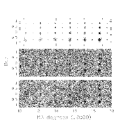
Figure 5: Distribution of simulated clusters with different richnesses and redshifts is shown in the top panel. The clusters are distributed such that the richness increases from left to right, and the redshift from bottom to top. The values are $\Lambda_{cl}=[20,40,70,110,160,220],\,z=[0.08,0.14,0.20,0.26,0.32,0.38,0.44,0.5]$. Every two columns correspond to a cluster of a given richness at eight different redshifts. The bottom panel shows these clusters embedded in a 25 $\mbox{deg}^{2}$ region of SDSS equatorial scan data. The middle panel shows the same clusters embedded in a uniform background generated by randomly repositioning the background galaxies shown in the bottom.

Artificial clusters with 6 different richnesses were embedded at 8 different redshifts each, giving a total of 48 clusters with different properties. The clusters were generated with a Schechter luminosity function ($\alpha=-1.1,\,M_{*}(r^{*})=-21.5$; Blanton et al. 2001) and a modified Plummer law radial profile ($r_{\mbox{max}}=1h^{-1}\mbox{Mpc},\,r_{\mbox{core}}=0.1r_{\mbox{max}}$; see Eq. (3)). Each cluster, properly normalized according to its richness $\Lambda_{cl}$, was placed at the corresponding redshift and then trimmed to the survey magnitude limit ($r^{*}=21$). The ($g^{*}-r^{*}$) color for each galaxy was assigned characteristic for a cluster at each redshift (as shown in Fig. 2). The insertion of simulated cluster galaxies increased the total number of galaxies in the 25 $\mbox{deg}^{2}$ region by 7%, to $105,600$ galaxies in total. The upper panel of Figure 5 shows the distribution of the 48 artificial clusters over a $10\times 2.5$ deg area (the parameters of the clusters themselves are given in the figure caption), and the resulting distribution when inserted into our uniform background is shown in the middle panel.

All three cluster finding algorithms (MF; AMF; VTT) were first run on this distribution of clusters in a uniform background of galaxies. The goal for this was to test each algorithm in the simplest case, and to find a reasonable detection threshold for each of them that maximizes the number of successful detections, while keeping the false detection rate minimal. Although this uniform background case is far from realistic, it has the advantage of unambiguously recognizing false detections. However, note that the number of clusters inserted and their distribution of $z$ and $\Lambda_{cl}$ are arbitrary. Thus, neither the fraction of false detections nor the absolute value of the recovery fraction that we quote below have physical significance; it is the relative values for different algorithms that should be noted.

Figure 6 shows the detection efficiencies for all three algorithms; each panel shows the number of successfully recovered clusters (solid curve) and the number of false detections (dotted curve) for one of the algorithms as a function of the detection threshold for the 48 clusters inserted into the uniform background. As the detection thresholds are decreased (going rightward in each panel of Figure 6), the number of successful detections increases, but naturally the rate of false detections due to Poisson statistics increases as well. Beyond a certain threshold value, the number of false detections start to increase extremely rapidly, while the number of successful detections only increases slowly; this implies a large drop in efficiency. Figure 7 shows this in another way, plotting the rate at which the number of successful detection increases as a function of the number of false detections for all three algorithms. We thus find a cut at which the success rate starts to flatten out with respect to the false detection rate; the vertical dotted line in Figure 7 shows an appropriate choice drawn just after the steepest part of the efficiency curve. This cut gives 14 false detections over 25 $\mbox{deg}^{2}$ for all three methods, $0.56\mbox{deg}^{-2}$, an acceptable level given the expected surface density of real systems ($>5\mbox{deg}^{-2}$; see Paper II). The vertical dashed lines in each panel of Figure 6 also show this cut, corresponding to $\sigma_{cut}=5.5$ for the MF and ${\cal L}_{cut}=210$ for the AMF. For the VTT the line indicates $N_{cut}=9$ (with a constant density contrast cut of $\delta_{c}=3$). We will refer to this cut in subsequent sections as the detection limit chosen for the uniform background case (note that $\sigma_{cut}$ will be slightly lower for the final results; §4.1). As Figure 7 demonstrates, of all methods, the MF is the most efficient in recovering clusters for a given number of false detections.

The additional clusters detected by the MF are clusters with a weaker signal (low $\Lambda_{cl}$, high $z$), as seen in Figures 8 a and b. These results are obtained using the cuts determined above. Although the AMF (crosses in Figure 8a) should in principle converge to the MF (squares in Figure 8a) in the 2-D case, they differ for weak clusters due to the fact that their peak selection method in the final step is done differently (refer to §2.1; Table 1). The parameter evaluation, on the other hand, is most accurate with the AMF fine filter. Figures 8 c and d show the input parameters for the clusters, $z$ and $\Lambda_{cl}$, plotted against the parameters evaluated by the AMF fine filter. They include the additional clusters found by the MF. The MF $z$ estimates show a factor of $\sim 1.5$ increase in standard deviation for higher redshift clusters ($z>0.25$), which translates into a larger deviation in $\Lambda_{cl}$ as well, by a similar amount. This result thus calls for a marriage of the two algorithms in order to maximize the efficiency of the final result. We have therefore adopted the following hybrid method for the final Matched Filter based cluster finder (HMF: Hybrid Matched Filter),

           $\bullet$ First the MF creates likelihood maps.
           $\bullet$ We threshold at $\sigma_{det}=\sigma_{cut}$ according to the MF to choose final cluster candidates.
           $\bullet$ Finally, we evaluate the AMF fine filter on these cluster positions to determine $\Lambda_{cl}$ and $z_{est}$.

We use this recipe as the standard Matched Filter method throughout the rest of this paper.

3.3 Monte Carlo with a “Realistic” Background

The previous test, using a uniform background, allowed us to determine the detection threshold necessary to minimize false detections due to projections in random fields. We need to apply a realistic background in order to get an accurate determination of the selection function, including the effect of large-scale structure and cluster projection along the line-of-sight. In relatively shallow surveys like the APM or the EDSGC the cluster detection efficiency has been shown to depend significantly on the local background density (see BNP00). The SDSS is considerably deeper ($z\sim 0.5$ compared to $z\sim 0.2$) and therefore this effect should be less dramatic, due to projection in 2D of the real large-scale structure. Nevertheless as the lower panel of Figure 5 shows, the SDSS galaxy distribution is still far from uniform, and the effect of large-scale structure on the selection needs to be quantified.

We now place the same set of simulated clusters on the real SDSS distribution as shown in the lower panel of Figure 5. The effect of the real background is immediately noticeable even by eye; the low richness clusters ($\Lambda_{cl}\leq 40$) are nearly washed out and the intermediate richness clusters ($\Lambda_{cl}=70,110$) start to blend in with the clumpy background.

The 48 simulated clusters with the properties given in Figure 5 were inserted into the data at random positions (unlike the grid distribution in the lower panel of Figure 5), but avoiding overlap with one another. Both the HMF and the VTT were run on this catalog. This was repeated 100 times. We use the results to test both the detection and recovery of clusters, and the evaluation of their parameters, $z$ and $\Lambda_{cl}$. In the next section we discuss the results from these tests in three parts. First, we study the effect of the imposed detection limits; second, we evaluate the selection function; and finally we examine the dependence of the detection efficiency and the recovered parameters on the local background.

4 Results

4.1 Detection Limits

A set of clusters embedded in a uniform background distribution is an ideal case. In the real universe, non-uniformity comes in many forms: from large scale modulations (great wall, voids etc.) down to small scale fluctuations (e.g., compact groups, close pairs and triplets etc.), in addition to actual clusters of galaxies. It is mainly the small scale features aided by projection that will cause the false-positive rate to increase. Therefore, the false detection rate that was determined with the uniform background ($0.56/{\mbox{deg}}^{2}$ for $\sigma_{cut}=5.5$ and $N_{cut}=9$) can be regarded as a lower limit for those thresholds in a realistic background. In addition, the structure exhibited on a range of scales diminishes the contrast of real clusters, making them more difficult to recover. This implies that these detection thresholds are upper limits on what they should be in the real universe. As we will see below, the detection threshold has to be set lower with a realistic background in order to recover a similar range of clusters.

For each cluster finder, we determine how many of the clusters that were detected in the uniform background case (with the corresponding detection thresholds $\sigma_{cut}=5.5$ and $N_{c}=9$; see Figure 8), were also recovered in each Monte Carlo realization with the SDSS galaxy background. This recovery ratio was evaluated for different detection thresholds, and averaged over all realizations. Figure 9 shows the results for both the HMF and the VTT, for a range of detection thresholds that are equivalent to those used in Figure 7. This recovery ratio (relative to the uniform background case) changes quite rapidly as a function of $\sigma_{cut}$ for the HMF, but stays rather robust as a function of $N_{cut}$ for the VTT. This comparison can be misleading since there is no formal correspondence between $N_{cut}$ and $\sigma_{cut}$. However, as noted above, these ranges are calibrated to yield approximately the same number of false detections in a uniform background distribution (c.f., Fig. 6). Given this relation as a yardstick, the noticeable difference in the slope of the two curves suggests that the Matched Filter algorithm results will be more sensitive to the detection threshold that is chosen, while a sample based on the VTT is robust to the exact value of $N_{cut}$. This implies in addition, that the Matched Filter is more subject to the effects of a non-uniform background, i.e., the detection efficiency is affected by the background distribution.

This argument is further supported by the lower recovery rate of the HMF shown in Figure 9 at the thresholds of $\sigma_{cut}=5.5$ for the HMF and $N_{cut}=9$ for the VTT (dotted lines; where both algorithms yielded 14 false detections in the uniform background case). Thus the detection efficiency of the HMF appears to be more affected by a non-uniform background than is the VTT. Indeed, this is not too surprising as the Matched Filter algorithm explicitly assumes a uniform background in its model. In order for the HMF to achieve the same recovery rate as the VTT, the detection threshold would need to be lowered to a value of $\sigma_{cut}\sim 4.7$ (which greatly increases the number of false detections, this would yield $\sim 60$ false detections in a uniform background; Fig. 6). These fractional recovery rates refer to the sample of 48 clusters over their entire range of $z$ and $\Lambda_{cl}$; hence it does not apply to an observed sample of clusters with a true richness function distribution. The clusters that are missed in the selection are those at the weaker end of the distribution of signal, which are the most abundant in the universe (i.e., poor, distant), therefore the gap between the recovery fractions shown above could be even larger for a more realistic configuration.

These result do not immediately mean, however, that the VTT does better overall. Recall from Figure 6 that the HMF was more efficient in recovering clusters in the uniform background to begin with. Given the right choice of detection thresholds we show that their performances are in fact similar in the end. Figure 10 shows the absolute recovery fraction of inserted clusters, rather than that relative to the uniform background (Fig. 9), for both the HMF (solid) and the VTT (dashed). This is shown in four different subgroups in cluster parameter space: low $z$, low $\Lambda_{cl}$ (lower left); high $z$, low $\Lambda_{cl}$ (upper left); low $z$, high $\Lambda_{cl}$ (lower right); and high $z$, high $\Lambda_{cl}$ (upper right). For clusters with the strongest signals (rich and nearby), both algorithms agree well with very high efficiencies, constant with respect to the detection thresholds. For clusters with weakest signals (poor, high $z$) both methods have very low recovery rate. Apart from the rich nearby regime, the HMF indeed shows slightly lower efficiencies than the VTT for the thresholds determined above ($\sigma_{cut}=5.5$, $N_{cut}=9$) suggesting a drop in efficiency due to the presence of a non-uniform background. However, the slopes of the HMF efficiency curves are much steeper, and allow us to bring up the detection efficiency easily to the VTT performance level, by lowering the detection threshold slightly to $\sigma_{cut}=5.2$. This naturally increases the false detection rate of the HMF in the uniform background case (refer to Fig. 6) by approximately 80% to $1\,\mbox{deg}^{-2}$, but as it is less than 20% of the expected surface density of real clusters (Paper II) we adopt this new value for $\sigma_{cut}$ as appropriate for selecting clusters from the SDSS imaging data. The final detection thresholds determined for both algorithms, $\sigma_{cut}=5.2$ and $N_{cut}=9$, are shown as dotted lines in Figure 10, indicating that the performance of the two algorithms is very similar.

4.2 Cluster Selection Function

With these detection thresholds, we now assess the overall performances of both cluster finders for these values in more detail, an important task for any study that requires a complete sample. We present selection functions evaluated from the fraction of clusters in each redshift and richness class that are recovered in the Monte Carlo simulations (using a realistic background). These selection functions for the HMF and the VTT are shown in Figures 11 and 12 with $\sigma_{cut}=5.2$ and $N_{cut}=9$, respectively. The two methods are qualitatively similar in terms of their overall performances; for clusters with $\Lambda_{cl}\geq 70$, over 80% are recovered to redshift $z\sim 0.45$, falling off rapidly as one goes to $z\sim 0.5$. There are still slight differences; the HMF does better in the high $\Lambda_{cl}$ intermediate $z$ ($0.2\lower 2.15277pt\hbox{$\;\buildrel<\over{\sim}\;$}z\lower 2.15277pt\hbox{$\;\buildrel<\over{\sim}\;$}0.4$) domain, while the VTT seems to perform slightly better for clusters with low $\Lambda_{cl}$ and low $z$ ($z\lower 2.15277pt\hbox{$\;\buildrel<\over{\sim}\;$}0.2$). This can be explained in terms of the generous C-M cuts adopted for the VTT, intended to account for possible fluctuations in the cluster color-magnitude properties. As a result, as one goes to higher redshift, where the C-M limits start to move in towards the core of the C-M distribution of normal galaxies (see Fig. 2), the population of galaxies that are rejected by this procedure reduces significantly, making this filtering less effective and therefore reducing the efficiency of recovering the clusters. At low redshifts $z\lower 2.15277pt\hbox{$\;\buildrel<\over{\sim}\;$}0.2$, on the other hand, it rejects most of the galaxy background, making the search most efficient. If we were to narrow these C-M limits, we might bias ourselves against clusters with unusual properties. This will be tested with real SDSS clusters by investigating their color-magnitude properties, to determine how tightly we can impose the limits without biasing the cluster selection.

We compare our selection functions to those of BNP00 (see their Fig. 2), evaluated for cluster detections in the EDSGC data. The redshift range probed with the EDSGC is much shallower ($z\lower 2.15277pt\hbox{$\;\buildrel<\over{\sim}\;$}0.15$; $b_{j}<20.5$, which corresponds roughly to $r<19$ for a typical elliptical galaxy) than that of the SDSS, however, they use the same Monte Carlo technique by inserting simulated clusters in the real data itself, making the comparison meaningful. Recall that the cluster detection completeness depends significantly on the use of different background distributions, as we have shown in Figures 9 and 10.

Figure 2 of BNP00 shows the selection function for four different richnesses as a function of redshift. Their richnesses correspond to $\Lambda_{cl}=10.15,20.3,40.6,\mbox{and}~{}81.2$, allowing a straightforward comparison to Figures 11 and 12. For $\Lambda_{cl}=20$ clusters, their efficiency drops from 70% to 40% over the redshift range of $0.05\leq z\leq 0.15$. Neither the HMF nor the VTT does significantly better for the same range of parameters, and beyond $z\sim 0.2$, clusters with $\Lambda_{cl}=20$ are virtually invisible even in the SDSS. However, for richer clusters, the SDSS clearly does better. For $\Lambda_{cl}=40$ clusters, BNP00 shows a steep drop in efficiency to $\sim 60\%$ at $z=0.15$, whereas the SDSS efficiencies stay at $\sim 80\%$ out to $z=0.2$. Similarly, the recovery of $\Lambda_{cl}=70$ clusters in the SDSS stays highly efficient ($\lower 2.15277pt\hbox{$\;\buildrel>\over{\sim}\;$}90\%$) and constant out to $z\sim 0.4$, while BNP00 efficiency for $\Lambda_{cl}=80$ clusters shows a clear drop from 100% to 80% already at $z=0.15$. The above comparison conforms to what we would expect: While going deeper in magnitude helps the recovery of clusters at higher redshifts, there is a limit in the cluster richness for which this is true. In other words, poor clusters are hard to find at high redshifts no matter what the depth of the survey is. Apart from those differences in the SDSS and EDSGC, the overall performances are qualitatively similar, which is reassuring given that our HMF is quite similar to their method.

4.3 Dependence on Local Background

The final issue we examine from this Monte Carlo experiment is the extent to which the results depend on the local background density. First, we look at the behavior of the detection efficiency at different locations. We divide our $2.5\times 10$ degree Monte Carlo region into $5\times 20$ subregions, $\sim 0.5$ deg on a side. This bin size is chosen to be large enough to get an appreciable number of clusters in each bin, for reliable statistics. We then count the number of background galaxies within each bin $N_{g}$ (excluding cluster galaxies), and evaluate the detection efficiency of clusters that fall into each bin. Figure 13 shows a scatter plot of the cluster detection efficiency as a function of the background density contrast $\delta_{g}=(N_{g}-\bar{N})/\bar{N}$. We have performed Spearman Rank Correlation tests (Press et al. 1990) and find that $r_{s}=-0.17,t=-1.72$ for the HMF and $r_{s}=-0.14,t=-1.39$ for the VTT, where $r_{s}$ is the Spearman rank-order correlation coefficient, and $t=r_{s}\sqrt{(N-2)/(1-r_{s}^{2})}$ which is distributed like a Student’s t distribution with $N-2$ degrees of freedom. This translates into correlations at only 5% and 8% confidence for the HMF and VTT respectively, confirming that neither method shows any significant correlation between their detection efficiency and the local background density. This is very encouraging, considering the unambiguous dependence that BNP00 have shown for their shallower sample (see Figure 3 in their paper). This suggests that our SDSS sample is deep enough to subdue the background fluctuations by projection effects, to a level that it does not affect the detection efficiency significantly. However, we have seen in §4.1 that the overall performance is still highly influenced by the presence of a non-uniform background, especially for the Matched Filter.

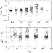
Figure 14: The input and output parameters evaluated by the HMF (equivalent to the AMF fine filter). The input values are discrete, $\Lambda_{cl}=[20,40,70,110,160,220],\,z=[0.08,0.14,0.20,0.26,0.32,0.38,0.42,0.5]$, and are therefore shown with a random scatter along the x-axes with a width of $\delta z=0.03$ and $\delta\Lambda_{cl}=20$, to facilitate visual identification.

We next investigate how HMF parameter evaluations depend upon the local background density. First, we show in Figure 14 the input and output values of $z$ and $\Lambda_{cl}$ for all detections in the Monte Carlo simulation. The distribution of $\Delta z$ is somewhat positively skewed, implying an overestimation of redshifts, which is pronounced as we go to higher $z$: the median values of $\Delta z$ are 0.007, 0.02 and 0.05 for input redshift ranges $0<z\leq 0.2,0.2<z<0.35$ and $z>0.35$, respectively. Also, half of the clusters with input redshifts $z\lower 2.15277pt\hbox{$\;\buildrel>\over{\sim}\;$}0.4$ are recovered with $z$ estimates at the upper $z$ limit ($z=0.5$). This trend was noted in the Matched Filter algorithm by P96, which usually happens with weak signals (poor and/or high redshift clusters), or in the field where there are no clusters, where the number-magnitude distribution of the background is such that the cluster likelihood calculated yields a monotonically increasing function with redshift. This could possibly be remedied by tweaking the input luminosity function to avoid such a trend in the likelihood function (e.g., flatter faint end slope), but this could bias parameter estimation in other ways, and we will not pursue this here.

We also find that the overestimation of redshift is amplified by the use of a non-uniform background. We have carried out the experiment of running the HMF on a given set of simulated clusters in both a uniform and a clustered background. We find that using the real background indeed increases the median redshift by about $10-15\%$, but also creates a long tail of under-estimated redshifts. We suggest that this is partly due to real clusters in the data that intercept the inserted clusters, thus affecting the output redshifts. The other concern pertains to the centroid of recovered clusters. While we may recover unbiased values exactly at the input center, the recovered clusters are always somewhat “offset” from the real center, and this could lead to some systematic effects. We thus repeated the Monte Carlo simulation using the true centers and the recovered centers, and found no sigificant systematic bias in the richness between the two runs. However, we do find that the number of clusters falsely estimated to be at $z=0.5$ was reduced by $\sim 15\%$ with the true centers.

The $\Lambda_{cl}$ input and output values are tightly correlated and do not show much systematic effects, but there is an extended tail of clusters with overestimated $\Lambda_{cl}$. These are the clusters that were falsely assigned to $z=0.5$, which boosts the estimated $\Lambda_{cl}$ to make up for the loss of galaxies beyond the magnitude limit. In what follows, we have left out all detections with $z_{est}=0.5$ to avoid such complications.

For each cluster recovered by the HMF, Figure 15 shows the difference between the input value and recovered value of $z$ and the ratio of the input and output values of $\Lambda_{cl}$, plotted against the density contrast of the local background, $\delta_{g}$. The value of $\delta_{g}$ at each cluster position is evaluated from counts in cell statistics on the background with a radius of 5 arcmin. This radius is chosen to represent the immediate local background of a cluster ($\sim$ 1 Abell radius at the median redshift of 0.2), much smaller than what was used for Figure 13, $(0.5\mbox{deg})^{2}$, where the bin was kept large in order to contain enough clusters to do statistics. The figure shows a slight correlation between the parameters and the local background density contrast. This is to some degree expected, since the model assumes a uniform background, therefore, a higher background density results in a higher estimation of richness $\Lambda_{cl}$, and vice versa. The redshift dependence shown in the lower panel of Figure 15 is due to the way in which the evaluation of the two parameters $z$, $\Lambda_{cl}$ are correlated. There are two effects operating. If the redshift is overestimated, then the angular extent of the cluster ($r_{\mbox{max}}$), within which $\Lambda_{cl}$ is calculated, is underestimated, resulting in a underestimated value of $\Lambda_{cl}$. However, if the redshift is overestimated, the value of $\Lambda_{cl}$ is over-compensated for the loss of galaxies fainter than the survey limit, but this effect is only significant near the faint limit of the survey (at the high-$z$ limit). Since the majority of recovered clusters are those at lower redshifts, the results exhibit an anti-correlation between the evaluated $z$ and $\Lambda_{cl}$. Figure 15 also demonstrates that most of the outliers in the parameter evaluations are high redshift clusters ($z>0.3$), shown as circles in the scatter plot.

5 Discussion and Summary

We have presented a comparison of three cluster finding algorithms which are being used to define a cluster catalog from commissioning data of the Sloan Digital Sky Survey. The three algorithms are two Matched Filter Algorithms (MF and AMF), and the Voronoi Tessellation Technique (VTT) which is introduced in its current form in this paper. By applying both Matched Filters on the same galaxy distribution, we have found that the MF is more efficient in locating the clusters, whereas the AMF evaluates the cluster parameters more accurately. This has motivated us to put forward a hybrid method (HMF) which uses the MF to select clusters and the AMF to evaluate the redshifts and the richnesses for those clusters.

The MF is more efficient in selecting clusters than the AMF is because its thresholding method is redshift dependent. The AMF locates peaks in redshift space first, and selects candidates with a signal above a prescribed threshold regardless of the redshift. On the other hand, the MF selects cluster candidates from peaks in the likelihood map of each assumed redshift; those lying above a threshold that is newly determined from each map. As similar clusters at different redshifts will have very different signals (weakening as one goes to higher $z$), it is not surprising to find that a redshift-dependent cut results in a better performance. Hence in future work, the AMF should be modified to adopt the peak selection procedure of the MF for better performance, in order to make use of the further advantages in the AMF (e.g., using three dimensional information and a parallelization scheme; Kepner & Kim 2000).

In the VTT method we have applied a filter in color-magnitude space to select galaxies that are most likely members of clusters at a certain redshift. This greatly enhances their contrast relative to the background. This idea is in principle yet another example of a matched filter; this time in color-magnitude space, although it is not a maximum likelihood method like the MF or the AMF. There are a number of existing algorithms that efficiently use this color-magnitude relation as a filter, but are more restrictive: the red-sequence method of Yee & Gladders (1999; Gladders & Yee 2000) and the maxBCG technique (also applied to the SDSS) of Annis et al. (2001). While using a restrictive color-magnitude relation could enhance the efficiency quite a bit, it is also likely to suffer from selection biases, such as missing clusters with significant blue populations of galaxies, namely, the Butcher-Oemler (1984) clusters.

Our current C-M filter for the VTT is generous, so that we can focus on the differences from the Matched Filter algorithms, where a specific cluster model is used. These differences will be further discussed in Paper II with real clusters; in the current paper we investigate the performance of this new method only with simulated clusters that exactly follow the spatial and luminosity profile assumed by the Matched Filter. Despite this advantange for the MF, the VTT has a similar selection function and better false positive rate compared to the MF, which points to the power of the technique, and suggests that photometric redshifts (which use color information) will significantly improve the performance of the AMF.

A Monte Carlo test for the HMF and the VTT was carried out with simulated clusters inserted in $25\mbox{deg}^{2}$ of SDSS background. We found that the HMF shows a larger drop in detection efficiency in the presence of a non-uniform background than does the VTT. This effect may be due not only to the non-uniformity, but also to overlapping foreground and background clusters in the data, which can cause some of the inserted clusters to be overlooked. This effect is roughly 15% for Abell richness class $\geq 0$ clusters in the redshift range of our interest, if we assume a random distribution of clusters. The VTT uses color information (although generous) that provides stability against such contamination, while the HMF assumes a uniform background and hence is affected more by this non-uniformity. Thus using a proper model of the background as a function of position can further improve the efficiency of the HMF (Lobo et al. 2000).

We have determined appropriate detection thresholds for the final cluster catalog that is to be drawn from the SDSS data itself. These thresholds are: $\sigma_{cut}=5.2$ and $N_{cut}=9$ for the HMF and the VTT respectively. These values give a reasonable recovery fraction; only 15% of clusters detected in the uniform background case are not recovered with the realistic background, while the lower limit on false detections, being a small fraction of the expected surface density of real systems, is acceptable ($1\mbox{deg}^{-2}$ for the HMF and $0.56\mbox{deg}^{-2}$ for the VTT).

The selection functions for both algorithms were evaluated using these detection thresholds. The performance of both methods are very similar, although the VTT efficiency tends to drop in the intermediate redshift range compared to the HMF, and is slightly better for lower redshift. Both methods are complete for rich clusters ($\Lambda_{cl}\geq 70$) up to $z\lower 2.15277pt\hbox{$\;\buildrel>\over{\sim}\;$}0.4$. We compare our selections functions to those of BNP00, where a similar cluster finding technique was used to find clusters in shallower data. We find that the performances are similar for the very low richness clusters ($\Lambda\sim 20$), while the SDSS outperforms BNP00 by going deeper for the richer clusters ($\Lambda\geq 40$).

Finally, we have shown that the detection efficiencies of both the HMF and the VTT are nearly independent of the local density of the background, while the estimated redshift and richness from the HMF are only slightly biased as a function of the local background density.

In Paper II, we present the cluster catalog compiled from the SDSS data using these two methods, the HMF and the VTT. With this we will be able to test various properties of the algorithms using real clusters. Photometric redshifts for the SDSS, soon available, will significantly improve the AMF in particular. In future work, it should be very interesting to compare the above methods with other existing techniques, e.g., the maxBCG technique (Annis et al. 2001) that uses far more restrictive color-magnitude information than the VTT, Cut and Enhance (Goto et al. 2001) that uses the proximity in color-space as an enhancement method, or the Expectation Maximization algorithm (Nichol et al. 2000), which does not impose any model constraints at all. Different algorithms show different results mainly for the fainter clusters – poor or distant clusters – the regime where clusters are abundant but our understanding is poor. Their detection will inevitably depend on different aspects of the method that is used. If one were to explore the properties of cluster parameters such as the luminosity function or the density profile, using the Matched Filter that constrains these models a priori will be highly inappropriate; when exploring the density-morphology relation of clusters, one should avoid using any color constraints in their selection. Therefore, there will be no one technique ideal for all aspects of cluster science; each cluster catalog should be accompanied with a proper understanding of the nature of the detection method, so that it can be used for appropriate cluster studies.

Figure 1: Color-magnitude (C-M) diagrams of four different clusters. (a) and (b) are known Abell clusters, and plotted here are the data from only those galaxies with confirmed membership according to the ENACS (Katgert et al. 1998). All data are taken from SDSS photometry. (c) and (d) show C-M diagrams of new clusters found in the SDSS itself by the matched filter techniques. Both clusters were confirmed visually through 3 color ($g,r,i$) composite images and their redshifts ($z=0.219$ and $z=0.345$) were obtained by the SDSS spectroscopic survey (York et al. 2000). The circles represent galaxies within 1 $h_{70}^{-1}$Mpc of the detected center ($r=4.74^{\prime}$ and $r=3.45^{\prime}$) and the contours represent the C-M distribution of all galaxies from a 25 $\mbox{deg}^{2}$ region around the cluster. The thick solid lines in all four panels show the C-M filtering for the VTT (see text) at the corresponding redshifts, enclosing the region which most cluster galaxies inhabit for a given redshift. $g^{*}-r^{*}$ colors are from model magnitudes and $r^{*}$ is in Petrosian magnitudes.

Figure 2: The empirical color-magnitude limits used in the Voronoi Tessellation Technique displayed for a range of redshifts ($0.04\leq z\leq 0.5,\Delta z=0.02$). These limits are used as a filter to enhance the signal of clusters at a given redshift (see text and Eq. (9) & (11)). The large dots trace the evolutionary track of a bright red galaxy with a constant luminosity $M_{r^{*}}=-23$, intended to represent the Brightest Cluster Galaxy. Each C-M limit encloses one BCG, and the redshift range of the C-M limits are labeled. The dots alternate as filled and open for each redshift range labeled, for easy identification. The contours and the small dots show the C-M distribution of all galaxies in the SDSS survey (taken from a 150 $\mbox{deg}^{2}$ region of the SDSS commissioning data) for comparison.

Figure 3: Example of Voronoi Tessellation executed on the galaxy distribution around Abell cluster 957 (see Figure 1(a)). These are all galaxies with $r^{*}<21$. Each cell encloses one galaxy. The data presented here has a lower boundary in declination of $\delta_{\mbox{J2000}}=-1.25^{\circ}$, which is why the Voronoi Tessellation seems to diverge below. The filled dots mark galaxies with $\delta>3$ (see text), and the large circle has a radius of 1$h^{-1}$ Mpc at a redshift of $z=0.044$ ($r=26.4^{\prime}$). We do not find any significant overdensity of the filled dots around Abell 957 when using the entire distribution of galaxies.

Figure 4: Same as Figure 3, but the Voronoi Tessellation is evaluated only on the galaxies that satisfy the color-magnitude criteria used in the VTT. See the solid lines in Figure 1(a) or Figure 2 for these limits. Unlike Figure 3, the cluster is now strikingly enhanced by the filled dots, which denote galaxies with $\delta>3$ evaluated from this Voronoi map.

Figure 6: The number of successful detections (solid) and the number of false detections (dotted) as a function of the detection threshold for each cluster finding algorithm: MF (left), VTT (middle), and AMF (right). These results are from 48 clusters inserted into a uniform background (see middle panel of Fig. 5). The MF is more efficient in detecting clusters than the AMF, due to differences in the thresholding method. The vertical dashed line is drawn at the thresholds that yield 14 false detections in a uniform background of 25 $\mbox{deg}^{2}$; this corresponds to $\sigma_{cut}=5.5$, $N_{cut}=9$ and ${\cal L}_{cut}=210$, yielding maximum completeness while still keeping the false detection rate less than 10% of the expected surface density of real clusters. Note that for all three algorithms, the ranges shown for the detection thresholds are calibrated to yield similar numbers of false detections.

Figure 7: The number of successful detections as a function of the number of false detections, as the detection threshold is changed for all three algorithms, in the uniform background case. This is an alternative representation of the data in Figure 6. The ranges for the detection thresholds represented here are $7\geq\sigma_{cut}\geq 4.5$ for the HMF (solid), $13\geq N_{cut}\geq 5$ for the VTT (dashed) and $450\geq{\cal L}_{cut}\geq 160$ for the AMF (dotted). The vertical dotted line shows the cut for $\sigma_{cut}=5.5$, $N_{cut}=9$ and ${\cal L}_{cut}=210$, at which the rapid increase of success rate stops with respect to the number of false detections (same cut as in Fig. 6). For a given number of false detections, the MF is most efficient in recovering clusters in a uniform background.

Figure 8: The results for 48 clusters embedded in a uniform background, using the detection threshold from Figure 6 (see caption), which yields 14 false detections for each techniques. (a) The parameters of the recovered clusters by the MF (squares) and the AMF (crosses). The MF selection method is more sensitive to weaker signals, i.e., higher $z$ and lower richness. (b) The clusters that were recovered by the VTT. The VTT is also slightly less efficient than the MF but more efficient than the AMF. All three algorithms show similar recovery patterns. (c) AMF fine filter determination of redshift for MF selected clusters (squares in (a)), versus the input value. (d) Same as (c), for the richness measure, $\Lambda_{cl}$. (c) and (d) are equivalent to the results for the HMF (Hybrid Matched Filter; see text for details).

Figure 9: The recovery rate of clusters in our Monte Carlo experiment as a function of the detection thresholds $\sigma_{cut}$, $N_{cut}$ for the HMF (solid) and the VTT (dashed) respectively. These recovery rates are evaluated relative to the clusters that were detected in the uniform background case, i.e., the average fraction of those clusters recovered in 100 Monte Carlo realizations. The standard deviations between realizations are traced with thin lines. The range of $\sigma_{cut}$ and $N_{cut}$ shown here are coincident with the values that were used to plot Figure 7. The dotted lines show the performance for $\sigma_{cut}=5.5$ and $N_{cut}=9$, which are the values that were determined from the uniform background case (vertical lines in Fig. 6 and 7).

Figure 10: Similar to Figure 9, but this shows the absolute recovery rates of clusters in 4 different ranges of cluster parameters for the HMF (solid) and the VTT (dashed), averaged over 100 Monte Carlo realizations. The $1\sigma$ dispersion is traced with thin curves. Four different panels show those for poor low $z$ clusters (lower left), poor high $z$ clusters (upper left), rich low $z$ clusters (lower right), and rich high $z$ clusters (upper right). Both algorithms agree very well for clusters with the highest signals (rich, low $z$) but VTT does slightly better in general for the thresholds determined from the uniform background case: $\sigma_{cut}=5.5$ and $N_{cut}=9$. The dotted lines show where $N_{cut}=9$ for the VTT, and $\sigma_{cut}=5.2$ for the HMF, lowered to this value to match the performance of the VTT.

Figure 11: The selection function evaluated for the HMF ($\sigma_{cut}=5.2$) as a function of redshift for clusters with different richness measures $\Lambda_{cl}$. Both $z$ and $\Lambda_{cl}$ shown are the input values of the simulated clusters generated with a Schechter luminosity function using $M_{r}^{*}=-21.7$ and $\alpha=-1.1$, and a modified Plummer law profile with $r_{max}=1$$h^{-1}$ Mpc and $r_{c}=0.1$$h^{-1}$ Mpc.

Figure 12: The selection function evaluated for the VTT ($N_{cut}=9$), in the same Monte Carlo experiment as Figure 11.

Figure 13: The detection efficiency as a function of the local background density contrast. Each circle represents the average fraction of clusters that were detected amongst those that were inserted in each independent cell of area $(0.5\,\mbox{deg})^{2}$. The density contrast is $\delta_{g}=(N_{g}-\bar{N})/\bar{N}$, where $N_{g}$ is the number of background galaxies in each cell and $\bar{N}$ is the average number of background galaxies in all cells. The top panel shows the results for the HMF and the bottom for the VTT. The Spearman Rank-Order Correlation test confirms that neither distribution shows any correlation with the background density (see text).

Figure 15: The dependence of the parameters evaluated by the HMF (equivalent to the AMF fine filter), on the local background density contrast. Each point represents one cluster; the difference in the input and output values of $z$ and the ratio of input and output $\Lambda_{cl}$ are plotted against $\delta_{g}$ of the background galaxy distribution, evaluated within a circle of $r=5^{\prime}$ around each cluster. The distributions of the points are shown as histograms on the left. The crosses are clusters which have an input redshift $z\leq 0.3$, the circles are clusters with input redshift $0.3<z<0.5$. The outliers are mostly high redshift clusters whose signals are weaker.

Table 1: Summary of the Procedures for the Two Matched Filter Algorithms

Step	Original Matched Filter (MF)	Adaptive Matched Filter (AMF)
1	Input galaxy catalog [position, magnitude]	same
2	Evaluate ${\cal L}_{\mbox{coarse}}$ on a uniform grid for assumed $z_{i}$	Calculate ${\cal L}_{\mbox{coarse}}$ on a $z$-grid for a galaxy position $x_{i}$
3	Repeat step 2 for $i=0,n$ ($n=$ # of $z$ bins)	Repeat step 2 for $i=0,m$ ($m=$ # of galaxies)
4	Save all likelihood maps for all $z_{i}$’s	Save $z_{\mbox{coarse}}$ and ${\cal L}_{\mbox{coarse}}$ where ${\cal L}_{\mbox{coarse}}(z)$ is
		maximum, for all $x_{i}$’s
5	Calculate $\sigma$ for each local maximum within each
	map, register cluster candidates if $\sigma>\sigma_{\mbox{cut}}$
6	Combine all candidates from all $z_{i}$ maps, filter	Find $x_{i}$ with highest ${\cal L}_{\mbox{coarse}}$, register as a cluster,
	overlaps and define $z_{\mbox{est}}$ for each cluster	eliminate nearby $x_{i}$’s, repeat until ${\cal L}_{\mbox{coarse}}<{\cal L}_{\mbox{cut}}$
7		Rerun fine filter on cluster positions from step 6,
		determine $z_{\mbox{fine}}$ and $\Lambda_{\mbox{fine}}$
	Final Product : Cluster positions, $z_{\mbox{est}}$, $\Lambda_{cl}$, $\sigma_{\mbox{det}}$	Final Product : Cluster positions, $z_{\mbox{fine}}$, $\Lambda_{\mbox{fine}}$, ${\cal L}_{\mbox{fine}}$
	using $\sigma_{\mbox{det}}>\sigma_{\mbox{cut}}$	using ${\cal L}_{\mbox{coarse}}>{\cal L}_{\mbox{cut}}$

References

- (1) Abell, G. 1958, ApJS, 3, 211
- (2) Abell, G., Corwin, H., & Olowin, R. 1989, ApJS, 70, 1
- (3) Annis, J. et al. for the SDSS collaboration 1999, AAS, 195, 1202
- (4) Annis, J. et al. 2001 in preparation
- (5) Bahcall, N. 1988, ARA&A, 26, 631
- (6) Bahcall, N. et al. for the SDSS collaboration 2001, in preparation
- (7) Bahcall, N., & Cen, R. 1993, ApJ, 408, L77
- (8) Bahcall, N., Fan, X., & Cen, R. 1997, ApJ, 485, L53
- (9) Baum, W. A. 1959, PASP, 71, 106
- (10) Bautz, L. P. & Morgan, W. W. 1970 ApJ, 162, 149
- (11) Blanton, M. et al. 2001, AJ, 121, 2358
- (12) Bramel, D. A., Nichol, R. C., & Pope, A. C. 2000, ApJ, 533, 601 (BNP00)
- (13) Butcher, H., & Oemler, A. 1984, ApJ, 285, 426
- (14) Carlberg, R., Morris, S., Yee, H., & Ellingson, E. 1997, ApJ, 478, L19
- (15) Collins, C. A. et al. 2000, MNRAS, 319, 939
- (16) Dalton, G., Efstathiou, G., Maddox, S., & Sutherland, W. 1992, ApJ, 390, L1
- (17) Dalton, G., Efstathiou, G., Maddox, S., & Sutherland, W. 1994, MNRAS, 269, 151
- (18) Dressler, A. 1980, ApJ, 236, 351
- (19) Dressler, A. 1984, ARA&A, 22, 185
- (20) Dressler, A., Oemler, A., Couch, W. J., Smail, I., Ellis, R. S., Barger, A., Butcher, H., Poggianti, B. M., & Sharples, R. M. 1997, ApJ, 490, 577
- (21) Ebeling, H. 1993, Ph.D. Thesis, Ludwig Maximilians Universitat Munich (Germany)
- (22) Ebeling, H., & Wiedenmann, G. 1993, PhRvE, 47, 704
- (23) Eisenstein, D. et al. 2001, AJ, in press, astro-ph/0108153
- (24) Evrard, A. 1989, ApJ, 341, L71
- (25) Fioc, M., & Rocca-Volmerage, B. 1997, A&A, 326, 950
- (26) Gal, R.R., DeCarvalho, R.R., Odewahn, S.C., Djorgovski, S.G., & Margoniner, V.E. 2000, AJ, 119, 12
- (27) Gladders, M.D., López-Cruz, O., Yee, H.K.C. & Kodama, T. 1998 ApJ, 501, 571
- (28) Gladders, M.D., & Yee, H.K.C. 2000, AJ, 120, 2148
- (29) Goto, T. et al. 2001, AJ, submitted
- (30) Gunn, J. E., & Dressler, A. 1988, in Towards Understanding Galaxies at Large Redshift, Ed., R. Kron & A. Renzini (Kluwer Academic, Dordrecht), 29
- (31) Gunn, J. E. & Oke, J. B. 1975, ApJ, 195, 255
- (32) Gunn, J. E., Hoessel, J. G., Oke, J. B. 1986, ApJ, 306, 30
- (33) Hoessel, J. G., Gunn, J. E., & Thuan, T. X. 1980, ApJ, 241, 486
- (34) Hubble, E. 1936, The Realm of the Nebulae, Yale University Press
- (35) Huchra, J., Geller, M., Henry, P., & Postman, M. 1990, ApJ, 365, 66
- (36) Icke, V. & van de Weygaert, R. 1987, A&A, 184, 16
- (37) Katgert, P., Mazure, A., den Hartog, R., Adami, C., Biviano, A. & Perea, J. 1998, A&AS, 129, 399
- (38) Kawasaki, W., Shimasaku, K., Doi, M., & Okamura, S. 1998 A&AS, 130, 567
- (39) Kepner, J., Fan, X., Bahcall, N., Gunn, J., Lupton, R. & Xu, G., 1999, ApJ, 517, 78 (K99)
- (40) Kepner, J. V. & Kim, R. S. J. 2000, Data Mining and Knowledge Discovery, submitted, astro-ph/0004304
- (41) Kiang, T. 1966, Z.f. Astroph., 64, 433
- (42) Kim, R.S.J., Strauss, M.A., Bahcall, N.A., Gunn, J.E., Lupton, R.H., Vogeley, M.S., Schlegel, D. for the SDSS collaboration 2000, ASP Conference Series Vol. 200, Clustering at High Redshift Les Rencontres Internationales de l’IGRAP, ed. A. Mazure, O. Le Fèvre, V. Lebrun, P.422 (astro-ph/9912302)
- (43) Kim, R.S.J. et al. 2001, in preparation (Paper II)
- (44) Lahav, O., & Gull, S. F. 1989, MNRAS, 240, 753
- (45) Ling E.N. 1987, Ph.D. Thesis, Sussex Univ., Brighton (England)
- (46) Lobo, C., Iovino, A., Lazzati, D., & Chincarini, G. 2000, A&A, 360, 896
- (47) Lugger, P. M. 1984, ApJ, 278, 51
- (48) Lumsden, S., Nichol, R., Collins, C., & Guzzo, L. 1992, MNRAS, 258, 1
- (49) Lupton, R. H., et al. 2001, in preparation
- (50) Maddox, S. J., Efstathiou, G., Sutherland, W. J., & Loveday, J. 1990, MNRAS, 243, 692
- (51) Metcalfe, N., Godwin, J.G. & Peach, J.V., 1994, MNRAS, 267, 431
- (52) Nichol, R. C., Briel, O. G., & Henry, J. P. 1994, MNRAS, 267, 771
- (53) Nichol, R. C., Collins, C. A., Guzzo, L., & Lumsden, S. L. 1992, MNRAS, 255, 21
- (54) Nichol, R. C., Collins, C. A., & Lumsden, S. L. 2001, ApJS, submitted, astro-ph/0008184
- (55) Nichol, R. C., Connolly, A. J., Moore, A. W., Schneider, J., Genovese, C., & Wasserman L. 2000a, Proceedings from “Virtual Observatories of the Future” Ed. R. J. Brunner, S. G. Djorgovski, A. Szalay, astro-ph/0007404
- (56) Nichol, R. C., et al. 2000b, conference proceedings from “Mining the Sky” in Munich, Germany
- (57) Oemler, A. 1974, ApJ, 194, 1
- (58) Olsen, L. F. et al. 1999, A&A, 345, 681
- (59) Oukbir, J., & Blanchard, A. 1997, A&A, 317, 1
- (60) Peacock, P. J. E., & Dodds, S. 1994, MNRAS, 267, 1020
- (61) Petrosian, V. 1976, ApJ, 209, L1
- (62) Postman, M. & Geller, M. J., 1984, ApJ, 281, 95
- (63) Postman, M., & Lauer, T. R. 1995, ApJ, 440, 28
- (64) Postman, M., Lauer, T. R., & Oegerle, W. 2001, in preparation
- (65) Postman M., Lauer, T.R., Szapudi, I., & Oegerle, W. 1998, ApJ, 506, 33
- (66) Postman M., Lubin, L., Gunn, J. E., Oke, J. B., Hoessel, J. G., Schneider, D. P., & Christensen, J. A. 1996, AJ, 111, 615 (P96)
- (67) Ramella, M., Nonino, M., Boschin, W., & Fadda, D. 1999, in Observational Cosmology: The Development of Galaxy Systems, ed. G. Giuricin, M. Mezzetti, and P. Salucci, ASP conference series, 176, 108
- (68) Ramella, M., Boschin, W., Fadda, D., & Nonino, M 2001, A&A, 368, 776
- (69) Reichart, D. E., Nichol, R. C., Castander, F. J., Burke, D. J., Romer, A. K., Holden, B. P., Collins, C. A., & Ulmer, M. P. 1999, ApJ, 518, 521
- (70) Rood, H. J., & Sastry, G. N. 1971, PASP, 83 313
- (71) Schneider, D. P., Gunn, J. E., Hoessel, J. G. 1983, ApJ, 264, 337
- (72) Schuecker, P. & Böhringer, 1998, A&A, 339, 315
- (73) Scodeggio, M., Olsen, L. F., da Costa, L., Slijkhuis, R., Benoist, C., Deul, E., Erben, T., Hook, R., Nonino, M., Wicenec, A., & Zaggia, S. 1999, A&AS, 137, 83
- (74) Schechter, P. 1976, ApJ, 203, 297
- (75) Shectman, S. A. 1985, ApJS, 57, 77
- (76) Silverman, B. 1986, “Density Estimation for Statistics and Data Analysis”, pp 40-43, Chapman and Hall, New York
- (77) Stoughton, C. et al. for the SDSS collaboration 2001, in preparation
- (78) Stoughton, C., Annis, J., Tucker, D. L., Hashimoto, Y., McKay, T. A. & Smith, J. A., 1998, BAAS 192, 51.03
- (79) van de Weygaert, R., & Icke, V. 1989, A&A, 213, 1
- (80) Visvanathan, N. & Sandage, A. 1977, ApJ, 216, 214
- (81) Willick, J. A., Thompson, K. L., Mathiesen, B. F., Perlmutter, S., Knop, R. A., Hill, G. J. 2001, PASP, 113, 658
- (82) Yasuda, N. et al. for the SDSS collaboration 2001, AJ, in press, astro-ph/0105545
- (83) Yee, H. K. C., Gladders, M. D. & López-Cruz, O., 1999, ASP Conference Series, Vol. 191, Photometric Redshifts and the Detection of High Redshift Galaxies, Ed. R. Weymann, L. Storrie-Lombardi, M. Sawicki & R. Brunner, P. 166
- (84) York, D. et al. 2000, AJ, 120, 1579
- (85) Zabludoff, A. I., & Mulchaey, J. S. 1998, ApJ, 496, 39
- (86) Zwicky, F., Herzog, E., Wild, P., Karpowicz, M., & Kowal, C. 1961-1968, Catalog of Galaxies and Clusters of Galaxies, Vol. 1-6 (Pasadena: Caltech)