Analysis of the First Disk-Resolved Images of Ceres from Ultraviolet Observations with the Hubble Space Telescope

Abstract

We present HST Faint Object Camera observations of the asteroid 1 Ceres at near-, mid-, and far-UV wavelengths ($\lambda=3636$, 2795, and 1621 Å, respectively) obtained on 1995 June 25. The disk of Ceres is well-resolved for the first time, at a scale of $\sim 50$ km. We report the detection of a large, $\sim 250$ km diameter surface feature for which we propose the name “Piazzi”; however it is presently uncertain if this feature is due to a crater, albedo variegation, or other effect. From limb fits to the images, we obtain semi-major and semi-minor axes of $R_{1}=484.8\pm 5.1$ km and $R_{2}=466.4\pm 5.9$ km, respectively, for the illumination-corrected projected ellipsoid. Although albedo features are seen, they do not allow for a definitive determination of the rotation or pole positions of Ceres, particularly because of the sparse sampling (two epochs) of the 9 hour rotation period. From full-disk integrated albedo measurements, we find that Ceres has a red spectral slope from the mid- to near-UV, and a significant blue slope shortward of the mid-UV. In spite of the presence of Piazzi, we detect no significant global differences in the integrated albedo as a function of rotational phase for the two epochs of data we obtained. From Minnaert surface fits to the near- and mid-UV images, we find an unusually large Minnaert parameter of $k\approx 0.9$, suggesting a more Lambertian than lunar-like surface.

The Astronomical Journal, January 2002 (in press)

1 Introduction

In the latter part of the 18th century, the Titius-Bode law led scientists to believe there was a “missing planet” in the region between Mars and Jupiter. On January 1st, 1801 — the first day of the 19th century — Giuseppe Piazzi serendipitously discovered the first minor planet: 1 Ceres

Ceres is a G-type asteroid (Tholen, 1984; Barucci et al., 1987) that orbits the Sun with a 4.4 yr period, a semi-major axis of 2.7 AU, and an eccentricity of 0.097. It has a rotational period of 9.075 hours (Lagerkvist et al., 1989). Lebofsky et al. (1986) reported that thermal observations of Ceres before and after opposition indicate that it is a prograde rotator (i.e., the pole is in the ecliptic North). Ceres has an absolute magnitude of $H=3.32$, and a magnitude slope parameter $G=0.12\pm 0.02$ (Lagerkvist & Magnusson, 1990). Ceres has measured optical colors of $U-B=0.43$ and $B-V=0.72$, and a visual geometric albedo $\sim 0.10$ (Tedesco, 1989).

In this paper we present Hubble Space Telescope/Faint Object Camera (HST/FOC) observations, which are the first images to resolve the disk of Ceres sufficiently to detect surface features. We present the observations, an analysis of the photometric results, and we discuss a few tantalizing features suggested by the data. Though the images are not sufficient to provide definitive new results regarding such issues as pole position and composition (due to restricted temporal and wavelength coverage), they do provide a basis data set to direct further observations that should answer these questions.

2 Observations and Data Reduction

The observations we report here were made by HST with the FOC over a 5-hour period on 1995 June 25. Table 1 describes the observations.

Table 1: Summary of Observations

Data Set	Band	$\lambda_{\rm center}$	$\Delta\lambda$	Filters	Start Time	Exp. Time	Rotational
		(Å)	(Å)		(1995 Jun 25, UT)	(sec)	Phase $\phi$ (deg)
x2og0101t	mid-UV	2795	134	F4ND F275W F278M	10:02:56	716.5	0.00
x2og0102t	near-UV	3626	106	F6ND F342W F1ND F372M	10:22:47	910.5	14.19
x2og0103t	far-UV	1621	159	F175W F152M	11:29:33	896.5	58.26
x2og0104t	far-UV	1621	159	F175W F152M	11:49:28	1292.5	73.61
x2og0105t	mid-UV	2795	134	F4ND F275W F278M	13:05:58	1016.5	122.67
x2og0106t	near-UV	3626	106	F6ND F342W F1ND F372M	13:30:49	1001.5	139.01
x2og0107t	far-UV	1621	159	F175W F152M	14:42:34	896.5	185.87
x2og0108t	far-UV	1621	159	F175W F152M	15:02:29	1292.5	201.22

At the time of observations, the Sun-Ceres-Earth phase angle was $\alpha=19.4$ deg, producing an observed illuminated fraction of 97.2% of the disk of Ceres; the corresponding defect of illumination was 0.012 arcseconds.

Ceres’ heliocentric distance was $r=2.57$ AU and its geocentric distance was $\Delta=2.97$ AU. At this distance, one arcsecond equates to about 2150 km, so the 0.01435 arcsec width of one FOC pixel corresponded to a physical scale of 30.9 km on the surface of Ceres. As stated in the HST/FOC Instrument Handbook, the FWHM of the FOC PSF for the filters we used in these observations is approximately 0.03 arcsec, giving a Rayleigh criterion resolution of $\sim 0.024$ arcsec (the width of $\sim 1.7$ pixels) or a spatial resolution of $\sim 52$ km on the surface of Ceres. From previous estimates of its size, we expected Ceres to have an angular diameter of about 0.43 arcsec (the width of 30 FOC pixels), giving us over 700 FOC pixels covering the disk of Ceres. This is significantly better spatial resolution and sampling than has been obtained previously with ground-based adaptive optics observations (Saint-Pé et al., 1993; Drummond et al., 1998).

Our HST/FOC observations consisted of two sets of exposures in three wavelength bands: the far-UV (using a F175W+F152M filter combination; $\lambda_{c}=1621$ Å, $\Delta\lambda=159$ Å), the mid-UV (F275W+F278M; $\lambda_{c}=2795$ Å, $\Delta\lambda=134$ Å), and near-UV (F342W+F372M; $\lambda_{c}=3626$ Å, $\Delta\lambda=106$ Å). Neutral density filters were used in the two longer-wavelength observations to keep the count rates at reasonable levels. We selected these UV bands because compared to visible wavelengths they provide better resolution, ice diagnostics, and surface contrast to search for features.

The FOC images, obtained with the COSTAR optical correction (Jedrzejewski et al., 1994), were reduced in the standard STScI Routine Science Data pipeline, which performed flatfielding and geometric corrections. The resulting images have a field of view of $7.3\times 7.3$ arcsec² ($512\times 512$ pixels, with each pixel $14.35\times 14.35$ mas² in size). Figure 1 shows the four mid-UV and near-UV FOC images of Ceres we obtained. The far-UV images are not shown here because they do not contain sufficient signal for displaying the disk or detecting features. However, as we show later, there is sufficient signal in the far-UV images to measure total disk-integrated counts (and thus determine the far-UV flux) from Ceres, which we compare to the total fluxes in the other bands as a measure of Ceres’ UV color slope.

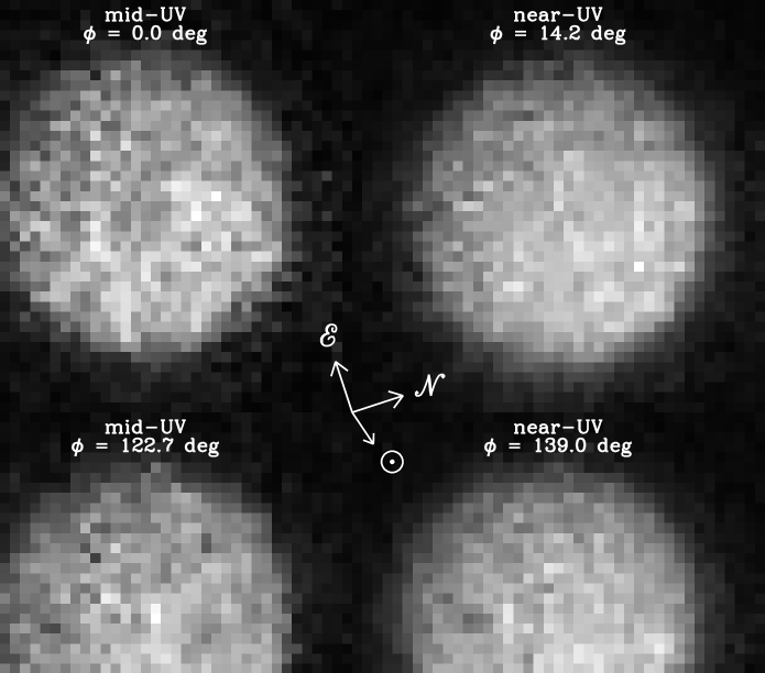
Figure 1: The mid-UV and the near-UV HST/FOC images of Ceres. Vectors show the direction of the Sun and the image orientation. The values for the relative rotational phase, $\phi$, of each image were calculated assuming a synodic rotational period of $P=9.075$ h (Lagerkvist et al., 1989). The images have been scaled such that they are all normalized to their peak pixel value (given in Table 3) for optimal contrast and ease of cross-comparisons. The Piazzi feature is near the center of the first mid-UV image ($\phi=0.0$ deg).

3 Discussion and Results

3.1 Regarding Shape and Pole Position

Ceres is the largest asteroid, but even after two hundred years of observations, its size is still in dispute. Estimates of the radius of Ceres have ranged from 391 km (Barnard, 1900) to 600 km (Dunham et al., 1974). Infrared Astronomical Satellite (IRAS) observations made in 1983 imply a radius of $457\pm 22$ km (Matson, 1986). More recent observations have considerably improved measurements to quoted uncertainties better than 1%, but with values differing by at least a few percent. The best direct size measurements available are the stellar occultation observations of Millis et al. (1987) and the adaptive optics images obtained by Saint-Pé et al. (1993) and Drummond et al. (1998). Millis et al. found projected equatorial and polar radii of $R_{1}=479.6\pm 2.4$ km and $R_{2}=453.4\pm 4.5$ km, respectively, and an equivalent radius of $R=\sqrt{R_{1}R_{2}}=466.3\pm 2.6$ km. Saint-Pé et al. find values that imply $R_{1}\sim 499$ km and $R_{2}\sim 469$ km, giving $R=484$ km. The Drummond et al. observations were rotationally resolved, allowing them to determine a fully triaxial shape with radii of $a=508$ km, $b=473$ km, and $c=445$ km, with uncertainties of about 5 km; their projected ellipse values are about 4% larger than those determined from the occultation observations of Millis et al..

We measured the disk center and the projected semi-major and semi-minor radii of Ceres by performing ellipse fits to each of the four good-signal HST images; this method was previously used to obtain shape parameters of the HST/WFPC2 images of Vesta (Thomas et al., 1997). Each image was scanned along columns or lines, depending on which is more nearly perpendicular to the limb. The resulting values were used to position a sharp edge along the scan; this was fit using the predicted disk brightness and a Gaussian smear from disk brightness to pixel brightness. (The predicted brightness on the disk was simply taken from the scan across the edge, where pixels that are 5–7 from the initial edge are averaged for an “on disk” value.) The position of the sharp edge was determined to 0.1 pixel-width by least squares matching of the predicted brightness along the scan to the actual one as a function of the modeled position of the sharp edge. For these images, obtained at modest phase angle, we performed a full-disk scan and corrected the down-sun (terminator) position to a predicted limb position of the raw data, and then ellipses were fit. Fits of the half ellipses (illuminated limb only) produced similar results, but have more uncertainty due to the greater uncertainty of the fit center. Table 2 gives the sub-Earth and sub-solar pixel coordinates in the FOC images resulting from our fits.

Table 2: Fitted Sub-Earth and Sub-Solar Pixel Coordinates

Data Set	Sub-Earth [$X_{c},Y_{c}$]	Sub-Solar [$X_{s},Y_{s}$]
x2og0101t	[197.80, 398.19]	[200.63, 393.95]
x2og0102t	[196.38, 396.50]	[199.21, 392.26]
x2og0105t	[192.41, 390.66]	[195.24, 386.42]
x2og0106t	[190.67, 389.53]	[193.50, 385.29]

Using this method, we obtain average values for Ceres’ illumination-corrected, projected semi-major and -minor radii of $R_{1}=484.8\pm 5.1$ km and $R_{2}=466.4\pm 5.9$ km, respectively, and an equivalent radius of $R=475.5\pm 3.9$ km. Since at the time of these observations the pole is within 1–18 deg of the plane of the sky for all of the published pole solutions, these radii of the projected ellipsoid are expected to be close to the true values. Our radii values are consistent with, though slightly larger than (by 1 to $2\sigma$), the sizes obtained from the occultation measurements by Millis et al. (1987), and are in better agreement with the adaptive optics values. Some of the differences could be due to the effect of differing rotational phase and sub-Earth latitude for the different observations. Observations taken at different epochs see the disk cross-section at different sub-Earth latitudes and longitudes, so comparisons are problematic since only the Drummond et al. (1998) observations provide an estimated 3-dimensional shape for Ceres. However, for an object rotating this slowly, the equilibrium shape is expected to be a Roche ellipsoid with axes of $a=b>c$, so the maximum projected axis is equal to the the equatorial axes; the minimum projected axis is between $a$ and $c$.

Using our projected radii we can determine the mean density of Ceres for a given mass. There have been several mass estimates for Ceres based on its perturbations on other asteroids (e.g., Schubart, 1974; Landgraf, 1988; Goffin, 1991; Sitarski & Todororovic-Juchniewicz, 1995; Viateau & Rapaport, 1998; Hilton, 1999; Michalak, 2000) and on Mars (Standish & Hellings, 1989). Table 1 shown by Michalak (2000) provides a complete list of mass estimates of Ceres, showing a range of masses from $6.7\times 10^{-10}{\cal M}_{\odot}$ (Schubart, 1970) to $4.3\times 10^{-10}{\cal M}_{\odot}$ (Kuzmanoski, 1996), though most of the values are within the range 4.6–$5.0\times 10^{-10}{\cal M}_{\odot}$. Millis et al. (1987) estimate a mean density of $\rho=2.7\pm 0.1~{}{\rm gm~{}cm}^{-3}$ using one of the higher mass estimates of $(5.9\pm 0.3)\times 10^{-10}{\cal M}_{\odot}$ (Schubart, 1974). For this mass, we obtain a similar density of $\rho=2.6\pm 0.2~{}{\rm gm~{}cm}^{-3}$. Using a lower mass estimate for Ceres of $(4.39\pm 0.05)\times 10^{-10}{\cal M}_{\odot}$ from Hilton (1999), our measurements imply a density $\rho=1.90\pm 0.05~{}{\rm gm~{}cm}^{-3}$.

The implications of these different density values are significant. Given the measured shape (specifically, the observed difference between the projected radii, $R_{1}-R_{2}$), the higher density is consistent with the assumption that Ceres is homogeneous and in hydrostatic equilibrium. However, at the lower density value, an object with the size and rotation period of Ceres would have a difference in the semi-major and -minor axes of $a-c\gtrsim 40$ km due to rotational flattening. The difference of the Millis et al. (1987) projected radii is $R_{1}-R_{2}=26.2\pm 5.1$ km, and the difference in our fit is even less: $18.4\pm 7.8$ km. Therefore, our results appear more consistent with the higher mass and density values: an object with the lower mean density value and the size and rotation period of Ceres should have greater flattening than is observed. However, if the lower density value is correct, then the observed lack of significant rotational flattening would imply that Ceres is not internally homogeneous. Another possible explanation for this discrepancy between the predicted and measured flattening would be that the pole position affected our measurement of the projected radii, such that the difference between the true axes, $a-c$, is significantly larger than our observed projected values, $R_{1}-R_{2}$; if that were the case, then Ceres could be homogeneous at the lower density. However, as discussed below, such a pole position is unlikely, again making our results more consistent with a higher mass value.

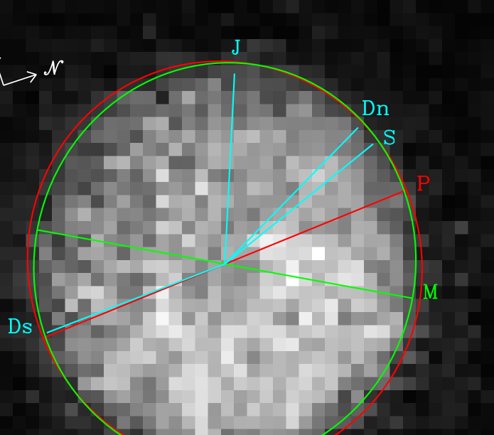
Figure 2: The first mid-UV image ($\phi=0.0$ deg) from Figure 1 showing the shape and pole position angles determined from various sources: “P” = this paper, “M” = Millis et al. (1987), “J” = Johnson et al. (1983), “S” = Saint-Pé et al. (1993), and “Dn” and “Ds” are the Drummond et al. (1998) north and south pole positions, respectively.

Because of the sparse rotational sampling of our HST data, we are not able to unambiguously track sufficient surface features to obtain a pole solution. If we assume that the slight flattening we find in the profile fit is due to rotation, then the best fit for our data put the projected pole angle at about 4 deg from North, with an uncertainty of roughly $\pm 15$ deg. We show our pole position angle and ellipse fit compared to those of other observations in Figure 2. These different values for the pole position show a range of over 90 deg. An initial analysis by Merline et al. (1996) of the motion of possible surface features seen in the FOC images suggested that the pole position might be more consistent with the Johnson et al. (1983) than with the Saint-Pé et al. (1993), but that result could not be convincingly re-established in our analysis. The uncertainties in our ellipsoidal fit do not allow combination with other results to constrain the pole. For example, the difference in projected axes reported by of Millis et al. (1987) of $R_{1}-R_{2}=26.2$ km could be reduced to agree with our value of 18.4 km by viewing an ellipsoid of $a=479.6,b=479.6,c=453.4$ km from 30 deg latitude. However, the published range of pole positions do not yield any viewing at greater than 18 deg latitude. Thus, we may only say the shape determined here, within our error bars, is consistent with the occultation results, but does not further constrain the spin pole.

3.2 Regarding Surface Characteristics

3.2.1 The Piazzi Feature

From examination of the images in Figure 1, no surface features could be easily tracked because of the large rotational phase difference between the pairs of FOC images within the same filter, and comparing images between different filters can lead to misidentifications due to differing reflectances at the different wavelengths.

However, while not trackable, there is one noticeable feature we are compelled to discuss. This is a significantly large, roughly circular, and centrally darkened spot, which appears face-on in the center of the first mid-UV image (rotational phase $\phi=0.0$ deg; upper left image in Figure 1), and covers about 40 pixels. Using these same HST/FOC images, this feature was independently noted by Landis et al. (1998). Because of the low number of counts, this is clearly not an artifact of nonlinear or wrapped count effects. It also is not a blemish from one of the FOC reseau marks, which are $3\times 3$ pixels in size (smaller than this feature); a map of the reseau marks shows that none are closer than $\sim$27 pixel-widths from the center of the disk of the Ceres image.

To determine the reality of this feature, we compared the average number of counts per pixel within the feature (allowing the radius and center point to vary) to the average number of counts per pixel in an annulus outside of the measurement aperture. We also repeated the same measurements for a annular ring rather than a photometric aperture. The results of these measurements are shown in Figure 3 and give us the following parameters: (i) the center point has an albedo about 30% lower than in the region surrounding the feature, and it monotonically increases to the edge of the feature; (ii) the optimal diameter of the feature is 8 pixel-widths (consistent with our by-eye estimate of 7 pixel-widths), or about 250 km; and (iii) the center of the dark feature is roughly 0.5 and $-0.5$ pixel-widths in the X and Y directions, respectively, from the center of the disk image as determined from our limb fits described earlier.

Figure 3: The photometric profile of the “Piazzi” feature on the first mid-UV image ($\phi=0.0$ deg) from Figure 1. The solid lines show the average number of counts per pixel (thick line) and associated photometric uncertainty (thin lines) within a circular aperture as a function of aperture radius. Similarly, the dashed line shows the average number of counts within a 1-pixel-wide photometric annulus. The horizontal dotted lines show the average number of counts and associated errors in a region beyond the feature. Note the annular photometry of the feature matches this background value at a radius of $\sim$4 pixel-widths, which is our estimate for the mean radius of the feature.

We also used the Kolmogorov-Smirnov (K-S) test (Press et al., 1992) to examine the statistical significance of this feature. We generated a featureless model of Ceres based on the Minnaert surface fit discussed in Section 3.2.3 and added Poisson noise to that model. We generated a cumulative distribution function based on 1000 such random models, which was then used to compare to our data as well as to 1000 more individual noise models to determine the distribution of K-S statistics. Comparing the FOC image to the models indicates a significant ($\sim 6\sigma$) difference, implying that this feature is not likely due to random noise. To check that this difference is not just due to a poor model, we repeated the same tests after masking out the feature’s pixels in both the FOC image and in the models; in this case the data agreed well ($\sim 2\sigma$) with the models, indicating that the model is a good match to the image, and only the pixels in the area of this feature are statistically deviant. To test that this change was not just an effect of masking out pixels from the analysis, we masked out other portions of the disk, but in those cases, the difference between the data and model remained large ($\sim$ 5–9$\sigma$), again indicating that only the region containing the feature is statistically unique. As a final check, we ran all the same tests on the second mid-UV image (labeled “$\phi=122.7$ deg” in Figure 1). Since that image does not show any obvious feature, we would expect that the model would fit the data in all cases (whether we were using all pixels, or masking out any region) better than the 5–9$\sigma$ deviations found for the first image with the feature not masked out. We found that the data in the second image were indeed better fit to the model in all cases, typically at the 3–4$\sigma$ level (only one case had a $5\sigma$ deviation), but not as good a match as one might hope. This could indicate that the model does not fit the data for the second mid-UV image quite as well, or perhaps the feature had rotated to another area of the visible disk and, though not easily identifiable by eye, is still statistically significant. However, these tests indicate that the models fit reasonably well.

Although our analysis cannot determine the nature of this feature, i.e., whether it is a crater, an albedo spot, or something else, we believe its existence is sufficiently established (to be definitive, we need higher-resolution images with adequate time sampling to see the motion of surface features). With that in mind, we propose the name “Piazzi” for this feature, in honor of the discoverer of Ceres.

3.2.2 The Geometric Albedo

Table 3: Summary of Photometry

Data Set	Band	Exp. Time	PHOTFLAM	Counts		Flux	Geometric Albedo
		(sec)		Peak	Total	(erg s-1 cm-2 Å-1)
x2og0102t	near-UV	910.5	9.720899$\times 10^{-15}$	79.1	37793	4.035$\times 10^{-13}$	$0.0558\pm 0.0010$
x2og0106t	near-UV	1001.5	9.720899$\times 10^{-15}$	86.8	41088	3.988$\times 10^{-13}$	$0.0552\pm 0.0010$
x2og0101t	mid-UV	716.5	3.302684$\times 10^{-15}$	28.6	13152	6.062$\times 10^{-14}$	$0.0298\pm 0.0006$
x2og0105t	mid-UV	1016.5	3.302684$\times 10^{-15}$	42.5	18068	5.871$\times 10^{-14}$	$0.0288\pm 0.0006$
x2og0103t	far-UV	896.5	6.379518$\times 10^{-15}$	5.8	677	4.820$\times 10^{-15}$	$0.1238\pm 0.0128$
x2og0104t	far-UV	1292.5	6.379518$\times 10^{-15}$	4.9	468	2.310$\times 10^{-15}$	$0.0593\pm 0.0068$
x2og0107t	far-UV	896.5	6.379518$\times 10^{-15}$	4.8	575	4.089$\times 10^{-15}$	$0.1059\pm 0.0091$
x2og0108t	far-UV	1292.5	6.379518$\times 10^{-15}$	5.0	560	2.764$\times 10^{-15}$	$0.0710\pm 0.0069$

The albedo of Ceres was determined in the standard manner and our results calculated from the FOC data are given in Table 3. The geometric albedo is defined as:

$$p(\lambda,\alpha)=\frac{r^{2}\Delta^{2}}{R^{2}_{\rm obj}}\left[\frac{F_{\rm obj}(\lambda)}{F_{\sun}(\lambda)}\right]f_{\alpha}$$ (1)

where $r$ and $\Delta$ are the heliocentric (in AU) and geocentric (in km) distances of the object at the time of the observation (these values for Ceres are given in Table 3), $R_{\rm obj}$ is the object’s radius in km (we use on our measured equivalent radius of $R=475.5$ km), $F_{\rm obj}(\lambda)$ is the measured flux, and $F_{\sun}(\lambda)$ is the solar flux at 1 AU over the same bandpass. For $F_{\rm obj}$ we use the background-subtracted disk-integrated flux calculated from the aperture photometry measured total counts listed in Table 3. The appropriate UV solar flux for these observations was obtained from the UARS satellite UV spectrometer, and the spectrum was modified by the FOC instrument response function using the synphot tasks in iraf. The parameter $f_{\alpha}$ is the dimensionless correction for solar phase angle. The UV phase function for Ceres is unknown; for our analysis here, we will use the value of the visible phase function: $f_{\alpha}=2.56$, which was calculated using the equations of Bowell et al. (1989) with a phase angle of $\alpha=19.4$ deg and slope parameter of $G=0.12$ (Lagerkvist & Magnusson, 1990).

The albedo uncertainties quoted in Table 3 are $1\sigma$-values based on the uncertainties in the equivalent radius of Ceres and in the aperture photometry using a 0.29 arcsec (20 pixel-widths) radius aperture that has been sky-subtracted using the modal value in a sky annulus with radii of 0.43–0.72 arcsec (30–50 pixel-widths); the FOC absolute photometric error is roughly 10–15%.

Figure 4: The UV geometric albedo of Ceres determined from the HST observations using a phase correction factor of $f_{\alpha}=2.56$ in Equation  1. The triangles ($\triangle$) indicate data from the first epoch of observations, and the squares ($\square$) indicate data from the second epoch. The number by each point indicates the rotational phase, $\phi$, of that observation. $1\sigma$ error bars are plotted representing aperture photometry and equivalent radius uncertainties only; for the near-UV and mid-UV data the error bars are comparable to the size of the plotted symbols.

The albedo values and their uncertainties are plotted in Figure 4. Even within the lower limit uncertainties shown, the albedo at the mid- and near-UV wavelengths display no evidence of rotational phase dependent variation. However, the data do show that Ceres has a red color slope longward of the mid-UV (0.032 per 1000 Å for $\lambda\gtrsim 2800$ Å); Ceres has a red color slope (though not as steep) through the visible bands as well (Butterworth & Meadows, 1985). Even within the large uncertainties in the far-UV photometry, there is a significant blue slope ($-0.051$ per 1000 Å for $\lambda\lesssim 2800$ Å) from the far-UV to the mid-UV, indicative of a minimum around 2800 Å. This break in slope is consistent with the differing mechanisms for formation of features as discussed by Gaffey et al. (1989): absorption shortward of $\sim 2500$ Å results from electron-hole pair formation, whereas the longer wavelength ($\sim 2500$ to 3500 Å) absorptions are produced primarily by charge-transfer mechanisms. There is no sign of significant absorption due to water across the disk, as that feature would occur in the far-UV filter, and no significant drop is seen in that bandpass. However, this does not rule out the possibility of water ice at the poles.

Butterworth & Meadows (1985) analyze International Ultraviolet Explorer (IUE) spectra of Ceres combined with data at longer wavelengths to determine albedo values from 2100–10000 Å. Their values of $p\approx 0.05$ at near-UV wavelengths and $p\approx 0.03$ at mid-UV wavelengths are in excellent agreement with our results. Roettger & Buratti (1994) also provide albedo measurements of Ceres from IUE observations in the wavelength range 2450–3150 Å, which nicely brackets our mid-UV measurements. Their calculated albedo values range from $p=0.024$–0.030, with an interpolated value of $p=0.025\pm 0.001$ at our mid-UV wavelength (2795 Å) whereas our averaged value is $p=0.029\pm 0.001$. The small difference could be due to values used for the phase angle correction (as noted above, we use the visible phase function correction for these UV data). The agreement of these IUE values and our near-UV and mid-UV results give us additional confidence in the reality of the large blue slope we find in the far-UV. Roettger & Buratti (1994) point out that G-type asteroids have higher albedos than C-type asteroids in the visible, but the UV albedos of the two type are similar. However, our HST observations also provide the first published far-UV data of any asteroid, so we cannot compare the far-UV blue slope to any other asteroid observations in order to understand how unique is this feature.

3.2.3 The Minnaert Parameters

Since the FOC images typically resolve Ceres’ disk into over 700 sunlit pixels, we can calculate the incidence and emission angles for each pixel, and in principle determine the Minnaert parameter, $k$, for Ceres. In practice, the brightness measured at each pixel will be a combination of Ceres’ intrinsic albedo distribution as well as the surface’s scattering properties. We therefore compare full-disk solutions for $k$ for each of the near- and mid-UV images, which should give us results that are reasonably insensitive to surface albedo variations given the large number of illuminated pixels and having images of Ceres at different rotational phases.

The Minnaert law (Minnaert, 1941) is an empirical approximation describing scattering from a surface. It has the form:

$$I/F=B_{0}\mu_{0}^{k}\mu^{k-1},$$ (2)

where $\mu_{0}$ and $\mu$ are cosines of the angles of emission and incidence, respectively, and $B_{0}$ and $k$ are the two Minnaert parameters (central $I/F$ and limb darkening parameter, respectively). The parameter $k$ typically depends strongly on the phase angle, although for a Lambert surface $k=1$ for all phase angles. When fitting the model to the data, there is a correlation between $k$ and the estimated radius as discussed below; we use our effective radius value of $R=475.5$ km (equivalent to 15.4 pixel-widths), although the fact that Ceres’ disk is not circular contributes to the uncertainty in the result.

We performed fits to the data using two independent methods: the $\chi^{2}$ minimization used by Veverka et al. (1989) in their analysis of Voyager 2 observations of Uranian satellites, and fitting a linearized logarithmic version of Eq. 2. Both methods agree within the estimated 2$\sigma$ uncertainties; Table 4 shows the results of our fits. If we vary the radius by $\pm 10$ km, the fitted values of $k$ typically vary by $\pm 0.04$, which are on the order of the uncertainties of the fits listed in Table 4. The values for $B_{0}$ do not appear to be correlated with radius.

Table 4: Fit Results for Minnaert Coefficients

Data Set	Band	$B_{0}$	$k$
x2og0101t	mid-UV	$22.8\pm 0.9$	$0.89\pm 0.03$
x2og0102t	near-UV	$65.4\pm 2.5$	$0.90\pm 0.03$
x2og0105t	mid-UV	$32.1\pm 1.3$	$0.92\pm 0.04$
x2og0106t	near-UV	$71.4\pm 2.7$	$0.92\pm 0.03$

The limb darkening parameter, $k$, is typically a strong function of the phase angle at the instant the observations were made, e.g., see Fig. 4 of Veverka et al. (1989). Ceres’ phase angle was $\alpha=19.4$ deg in these observations. Regardless of the phase angle, however, Ceres’ limb parameter is quite high (around $k=0.9$) relative to $k$ values for Uranian, Galilean, and Saturnian satellites (Buratti, 1984; Veverka et al., 1989). The simplest interpretation is that Ceres scatters more like a Lambertian surface ($k=1$) than a lunar-like surface ($k=0.5$), which implies that much of the light we see from the surface of Ceres undergoes multiple reflections. Interestingly, Saint-Pé et al. (1993) find just the opposite in their infrared images: they find that the center-to-limb brightness profile in the $H$ and $K$ bands is better fit by a (lunar-like) flat disk than a Lambertian sphere. This disagreement could be the result of their lower resolution and/or possible surface reflectance differences between the IR and the UV wavelengths. Hestroffer & Mignard (1997) also find a lower value for the Minnaert parameter, $k=0.61$, using a technique of analyzing the signal modulation of Hipparcos Satellite data (Ceres is not resolved in their data). Although they use an average phase angle of $\alpha=18$ deg, a value similar to ours, they use the smaller IRAS-based radius, $R=456.5$ km, which would account for much of the difference (their $\Delta k/\Delta R\approx 0.092$ km^-1): using the radii values we find from our HST data, the calculations of Hestroffer & Mignard (1997) would yield values of $k=0.74-0.87\pm 0.05$, in better agreement with our results.

4 Conclusions

Our analysis of HST/FOC near-, mid-, and far-UV images of Ceres have produced the following results:

1. These are the first, well-resolved ($\sim 50$ km) images of Ceres.

2. We have made a detection of an apparently large, $\sim 250$ km diameter surface feature for which we propose the name “Piazzi”.

3. The semi-major and semi-minor axes are $R_{1}=484.8\pm 5.1$ km and $R_{2}=466.4\pm 5.9$ km, respectively, for the projected ellipsoid.

4. Disk-integrated photometry in the three bandpasses show that Ceres has averaged geometric albedo values of: $p=0.056$ in the near-UV, $p=0.029$ in the mid-UV, and $p=0.090$ in the far-UV. These values give a red spectral slope (0.032 per 1000 Å) from the mid- to near-UV, and a significant a blue slope ($-0.052$ per 1000 Å) shortward of the mid-UV. The relatively high albedo value in the far-UV implies there is no significant absorption due to ice across the disk.

5. We detect no significant global differences in the full-disk integrated albedo as a function of rotational phase for the two epochs of data we obtained.

6. From Minnaert surface fits to the near- and mid-UV images, we find an unusually large Minnaert parameter of $k\approx 0.9$, suggesting a more Lambertian than lunar-like surface.

It is clear that more such imaging observations are needed with better sampling of the rotation period to finally resolve the continuing, long-standing uncertainty in Ceres’ pole position, and to obtain more information on the intriguing Piazzi feature detected in these observations. Also, more sensitive observations in the far-UV should be obtained to search for surface ice on Ceres and map its distribution; the far-UV bandpass is well-matched to the strong water ice absorption near 1650 Å as seen both in laboratory data (e.g. Hudson, 1971) and in the rings of Saturn (Wagener & Caldwell, 1988). Such observations could be obtained with the next generation of HST imaging space instruments, allowing us to probe ever more deeply into the nature of this largest and longest known asteroid.

References

- Altenhoff et al. (1996) Altenhoff, W. J., Baars, J. W. M., Schraml, J. B., Stumpff, P., & Von Kap-Herr, A. 1996, A&A, 309, 953
- Barnard (1900) Barnard, E. E. 1900, MNRAS, 60, 261
- Barucci et al. (1987) Barucci, M. A., Capria, M. T., Coradini, A., & Fulchignoni, M. 1987, Icarus, 72, 304
- Bowell et al. (1989) Bowell, E., Hapke, B., Domingue, D., Lumme, K., Peltoniemi, J., & Harris, A. W. 1989, in Asteroids II, eds. R. P. Binzel, T. Gehrels, and M. S. Matthews (University of Arizona Press, Tucson), 524
- Buratti (1984) Buratti, B. J. 1984, Icarus, 59, 392