Computational aspects of astrophysical MHD and turbulence

Abstract

The advantages of high-order finite difference scheme for astrophysical MHD and turbulence simulations are highlighted. A number of one-dimensional test cases are presented ranging from various shock tests to Parker-type wind solutions. Applications to magnetized accretion discs and their associated outflows are discussed. Particular emphasis is placed on the possibility of dynamo action in three-dimensional turbulent convection and shear flows, which is relevant to stars and astrophysical discs. The generation of large scale fields is discussed in terms of an inverse magnetic cascade and the consequences imposed by magnetic helicity conservation are reviewed with particular emphasis on the issue of $\alpha$-quenching.

1 Introduction

Over the past 20 years multidimensional astrophysical gas simulations have become a primary tool to understand the formation, evolution, and the final fate of stars, galaxies, and their surrounding medium. The assumption that those processes happen smoothly and in a non-turbulent manner can at best be regarded as a first approximation. This is evidenced by the ever improving quality of direct imaging techniques using space telescopes for example. At the same time not only have computers become large enough to run three-dimensional simulations with relatively little effort, there have also been substantial improvements in the algorithms that are used. In fact, there is now a vast literature on numerical astrophysics. An excellent book was published recently by LeVeque et al. (1998) where both numerical methods and astrophysical applications were discussed in great detail. Most of the applications focused however on rather more ‘violent’ processes such as supersonic jets, supernova explosions, core collapse, and on radiative transfer problems, while hydromagnetic phenomena and turbulence problems where only touched upon briefly. Meanwhile, hydromagnetic turbulence simulations have become crucial for understanding viscous dissipation in accretion discs (Hawley, Gammie, & Balbus 1995), and for understanding magnetic field generation by dynamo action in discs (Brandenburg et al. 1995, 1996a, Hawley, Gammie, & Balbus 1996, Stone et al. 1996), stars (Nordlund et al. 1992, Brandenburg et al. 1996b), and planets (Glatzmaier & Roberts 1995, 1996).

Much of the present day astrophysical hydrodynamic work is based on the ZEUS code, which has been documented in great detail and described with a number of test cases in a series of papers by Stone & Norman (1992a,b). The main advantage is its flexibility in dealing with arbitrary orthogonal coordinates which makes the code applicable to a wide variety of astrophysical systems. The code, which is freely available on the net, uses artificial viscosity for stability and shock capturing, and is based on an operator split method with second-order finite differences on a staggered mesh. Another approach used predominantly in turbulence research are spectral methods (e.g. Canuto et al. 1988), which have the advantage of possessing high accuracy. Although these methods are most suitable for incompressible flows (imposing the solenoidality condition is then straightforward), they have also been applied to compressible flows (e.g. Passot & Pouquet 1987). As a compromise one may resort to high order finite difference methods, which have the advantage of being easy to implement and yet have high accuracy. Compact methods (e.g. Lele 1992) are a special variety of high order finite difference methods, but the truncation error is smaller than for an explicit scheme of the same order. Compact schemes have been used by Nordlund & Stein (1990) in simulations of solar convection (Stein & Nordlund 1989, 1998) and convective dynamos (Nordlund et al. 1992, Brandenburg et al. 1996b), for example.

The use of compact methods involves solving tridiagonal matrix equations, making this method essentially nonlocal in that all points are now coupled at once. This is problematic for massively parallel computations, which is why Nordlund & Galsgaard (1995, see also Nordlund, Galsgaard, & Stein 1994) began to use explicit high order schemes for their work on coronal heating by reconnection (Galsgaard & Nordlund 1996, 1997a,b). In their code the equations are solved in a semi-conservative fashion using a staggered mesh. This code was also used by Padoan, Nordlund, & Jones (1997) and Padoan, & Nordlund (1999) in models of isothermal interstellar turbulence in molecular clouds, and by Rögnvaldsson, Nordlund, & Sommer-Larsen (2001) in simulations of cooling flows and galaxy formation.

A somewhat different code was used by Brandenburg (1999) and Bigazzi (1999) in simulations of the inverse magnetic cascade, by Kerr & Brandenburg (1999) in work on the possibility of a singularity of the nonresistive and inviscid MHD equations, and by Sanchez-Salcedo & Brandenburg (1999, 2001) in simulations of dynamical friction. A two-dimensional version of the code modelling outflows from magnetized accretion discs has been described by Brandenburg et al. (2000). This code uses sixth order explicit finite differences in space and third order Runge-Kutta timestepping. It employs central finite differences, so the extra cost of recentering a large number of variables between staggered meshes each timestep is avoided.

Apart from high numerical accuracy, another important requirement for astrophysical gas simulations is the capability to deal with a large dynamical range in density and temperature. This requirement favors the use of non-conservative schemes, because then logarithmic variables can be used which vary much less than linear density and energy density per unit volume. Solving the nonconservative form of the equations can be more accurate than solving the conservative form. The conservation properties can then be used as an indicator for the overall accuracy.

In this chapter we concentrate on numerical astrophysical turbulence aspects starting with a discussion of different numerical methods and a description of the results of various numerical test problems. This is a good way of assessing the quality of a numerical scheme and of comparing with other methods; see Stone & Norman (1992a,b) for a series of tests using the ZEUS code. After that we discuss particular astrophysical applications including stellar convection, accretion disc turbulence and associated outflows, as well as the generation of magnetic fields (small scale and large scale) from turbulence in various astrophysical settings.

2 The Navier-Stokes equations

The discussion of magnetic fields will be postponed until later, because the inclusion of the Lorentz force in the momentum equation is straightforward. We begin by writing down the Navier-Stokes equations in nonconservative form and rewrite them such that the main thermodynamical variables are entropy and either logarithmic density or potential enthalpy. These variables have the advantage of varying spatially much less than for example linear pressure and density.

The primitive form of the continuity equation is

$${\partial\rho\over\partial t}=-\mbox{\boldmath$\nabla$}{}\cdot(\rho\mbox{\boldmath$u$}{}),$$ (1)

which means that the local change of density is given by the divergence of the mass flux at that point. The Navier-Stokes equation can be written as

$$\rho{{\rm D}{}\mbox{\boldmath$u$}{}\over{\rm D}{}t}=-\mbox{\boldmath$\nabla$}{}p-\rho\mbox{\boldmath$\nabla$}{}\Phi+\mbox{\boldmath$F$}{}+\mbox{\boldmath$\nabla$}{}\cdot\mbox{\boldmath$\tau$}{},$$ (2)

where ${\rm D}{}/{\rm D}{}t=\partial/\partial t+\mbox{\boldmath$u$}{}\cdot\mbox{\boldmath$\nabla$}{}$ is the advective derivative, $p$ is the pressure, $\Phi$ is the gravitational potential, $F$ is a body force (e.g., the Lorentz force), and $\tau$ is the stress tensor.

The Navier-Stokes equation is here written in terms of forces per unit volume. As argued above, if the density contrast is large it is advantageous to write it in terms of forces per unit mass and to divide by $\rho$. Before we can replace $p$ and $\rho$ by entropy and logarithmic density or potential entropy we first have to define some thermodynamic quantities.

Internal energy, $e$, and specific enthalpy, $h$ are related to each other by

$$h=e+pv,$$ (3)

where $v=1/\rho$ is the specific volume and $\rho$ the density. The specific entropy is defined by

$$T{\rm d}{}s={\rm d}{}e+p{\rm d}{}v,$$ (4)

where $T$ is temperature. The specific heats at constant pressure and constant volume are defined as $c_{p}={\rm d}{}h/{\rm d}{}T|_{p}$ and $c_{v}={\rm d}{}e/{\rm d}{}T|_{v}$, their ratio is $\gamma=c_{p}/c_{v}$, and their difference is ${\cal R}/\mu=c_{p}-c_{v}$, where ${\cal R}$ is the universal gas constant and $\mu$ the specific molecular weight.

In the following we assume $c_{p}$ and $c_{v}$ to be constant for all processes considered. Ionization and recombination processes are therefore ignored here, although this is not a major obstacle; see, e.g., simulations of Nordlund (1982, 1985), Steffen, Ludwig, & Krüß (1989), Stein & Nordlund (1989, 1998), Rast et al. (1993), and Rast & Toomre (1993a,b) where realistic equations of state have been used.

We now assume that $c_{p}$ and $c_{v}$ are constant, so internal energy and specific enthalpy are given by

$$h=c_{p}T\quad\mbox{and}\quad e=c_{v}T,$$ (5)

This allows us then to write the specific entropy (up to an additive constant) as

$$s=c_{v}\ln p-c_{p}\ln\rho.$$ (6)

The pressure gradient term in the momentum equation can then be written as

$${1\over\rho}\mbox{\boldmath$\nabla$}{}p={p\over\rho}\mbox{\boldmath$\nabla$}{}\ln p={\gamma p\over\rho}(\mbox{\boldmath$\nabla$}{}\ln\rho+\mbox{\boldmath$\nabla$}{}s/c_{p})=c_{\rm s}^{2}(\mbox{\boldmath$\nabla$}{}\ln\rho+\mbox{\boldmath$\nabla$}{}s/c_{p}),$$ (7)

where we have used

$$c_{\rm s}^{2}=\gamma p/\rho={\gamma p_{0}\over\rho_{0}}\exp[(\gamma-1)\ln(\rho/\rho_{0})+\gamma s/c_{p}]=c_{\rm s0}^{2}\left({\rho\over\rho_{0}}\right)^{\gamma-1}\exp(\gamma s/c_{p}),$$ (8)

where $c_{\rm s}$ is the adiabatic sound speed, and $c_{\rm s0}^{2}=\gamma p_{0}/\rho_{0}$.

With these preparations the evolution of velocity $u$, logarithmic density $\ln\rho$, and specific entropy $s$ can be expressed as follows:

$${{\rm D}{}\mbox{\boldmath$u$}{}\over{\rm D}{}t}=-c_{\rm s}^{2}(\mbox{\boldmath$\nabla$}{}\ln\rho+\mbox{\boldmath$\nabla$}{}s/c_{p})-\mbox{\boldmath$\nabla$}{}\Phi+\mbox{\boldmath$f$}{}+{1\over\rho}\mbox{\boldmath$\nabla$}{}\cdot(2\nu\rho\mbox{\boldmath${\sf S}$}{}),$$ (9) $${{\rm D}{}\ln\rho\over{\rm D}{}t}=-\mbox{\boldmath$\nabla$}{}\cdot\mbox{\boldmath$u$}{},$$ (10) $$T{{\rm D}{}s\over{\rm D}{}t}=2\nu\mbox{\boldmath${\sf S}$}{}^{2}+\Gamma-\rho\Lambda,$$ (11)

where $\mbox{\boldmath$f$}{}=\mbox{\boldmath$F$}{}/\rho$ is the body force per unit mass, $\Gamma$ and $\Lambda$ are heating and cooling functions, $\nu$ kinematic viscosity and ${\sf S}$ is the (traceless) strain tensor with the components

$${\sf S}_{ij}={\textstyle{1\over 2}}(u_{i,j}+u_{j,i}-{\textstyle{2\over 3}}\delta_{ij}u_{k,k}).$$ (12)

In the presence of an additional kinematic bulk viscosity, $\zeta$, the term $2\nu{\sf S}_{ij}$ under the divergence in eq. (9) would need to be replaced by $2\nu{\sf S}_{ij}+\zeta\delta_{ij}\mbox{\boldmath$\nabla$}{}\cdot\mbox{\boldmath$u$}{}$, and the viscous heating term, $2\nu\mbox{\boldmath${\sf S}$}{}^{2}$, in eq. (11) would need to be replaced by $2\nu\mbox{\boldmath${\sf S}$}{}^{2}+\zeta(\mbox{\boldmath$\nabla$}{}\cdot\mbox{\boldmath$u$}{})^{2}$.

Instead of using $\rho$ as a dependent variable an can also use the specific enthalpy $h$, which allows us to write the pressure gradient as

$$-{1\over\rho}\mbox{\boldmath$\nabla$}{}p=-\mbox{\boldmath$\nabla$}{}h+T\mbox{\boldmath$\nabla$}{}s.$$ (13)

This formulation is particularly useful if the entropy is nearly constant (or if the gas is barotropic, i.e. $p=p(\rho)$) and if there is a gravitational potential $\Phi$, so that the potential enthalpy $H\equiv h+\Phi$ can be used as dependent variable. In order to express eq. (10) in terms of $h$ we write down the total differential of the specific entropy,

$${\rm d}{}s/c_{p}={1\over\gamma}{\rm d}{}\ln p-{\rm d}{}\ln\rho={1\over\gamma}{\rm d}{}\ln h-\left(1-{1\over\gamma}\right){\rm d}{}\ln\rho,$$ (14)

so

$${{\rm D}{}\ln h\over{\rm D}{}t}=\gamma{{\rm D}{}s/c_{p}\over{\rm D}{}t}+(\gamma-1){{\rm D}{}\ln\rho\over{\rm D}{}t}.$$ (15)

Furthermore, $T\mbox{\boldmath$\nabla$}{}s=h\mbox{\boldmath$\nabla$}{}s/c_{p}$, and so the final set of equations is

$${{\rm D}{}\mbox{\boldmath$u$}{}\over{\rm D}{}t}=-\mbox{\boldmath$\nabla$}{}H+h\mbox{\boldmath$\nabla$}{}s/c_{p}+\mbox{\boldmath$f$}{}+\mbox{\boldmath$\nabla$}{}\cdot(2\nu\rho\mbox{\boldmath${\sf S}$}{}),$$ (16) $${{\rm D}{}s/c_{p}\over{\rm D}{}t}={1\over h}\left(2\nu\mbox{\boldmath${\sf S}$}{}^{2}+\Gamma-\rho\Lambda\right),$$ (17) $${{\rm D}{}H\over{\rm D}{}t}=\mbox{\boldmath$u$}{}\cdot\mbox{\boldmath$\nabla$}{}\Phi+\gamma h{{\rm D}{}s/c_{p}\over{\rm D}{}t}-c_{\rm s}^{2}\mbox{\boldmath$\nabla$}{}\cdot\mbox{\boldmath$u$}{},$$ (18)

where we have absorbed $\Phi$ in the potential enthalpy $H=h+\Phi$. In this formulation the density can be recovered as

$$\rho=\rho_{0}\left[\left(1-{1\over\gamma}\right)\left({h\over c_{\rm s0}^{2}}\right)\,e^{-\gamma s/c_{p}}\right]^{1/(\gamma-1)}$$ (19)

(in dimensional form) or, for $\gamma=5/3$ and in nondimensional form (where $\rho_{0}=p_{0}=c_{p}=1$),

$$\rho=(0.4h)^{1.5}\,e^{-2.5s}.$$ (20)

We shall use either of the two sets of the equations, (9)–(11) or (16)–(18), in some of the following sections, especially in connection with shock tests and stellar wind problems. In these cases the gravity potential $\Phi$ is important and it turns out that the potential enthalpy $H\equiv h+\Phi$ varies only very little near the central object even though $\Phi$ itself tends to become singular.

The heating and cooling terms ($\Gamma$ and $\Lambda$) are important for example in the case of interstellar turbulence which is driven primarily by supernova explosions which inject a certain amount of thermal energy ($\int\rho\Gamma{\rm d}{}V$) with each supernova explosion. MHD turbulence simulations of this type were performed recently by Korpi et al. (1999). At the same time there is cooling through various processes (e.g. bremsstrahlung at high temperatures) which transports energy either nonlocally via a cooling term $\Lambda(T)$, or locally via thermal conduction or radiative diffusion. In the radiative diffusion approximation we express $\Lambda$ as $-\rho^{2}\Lambda=\mbox{\boldmath$\nabla$}{}\cdot K\mbox{\boldmath$\nabla$}{}T$, where $K$ is the radiative conductivity which is in general a function of temperature and density. The radiative diffusivity (which has the same dimensions as the kinematic viscosity $\nu$) is given by $\chi=K/(\rho c_{p})$, so

$$-\rho\Lambda/(c_{p}T)={1\over\rho c_{p}T}\mbox{\boldmath$\nabla$}{}\cdot\rho\chi c_{p}\mbox{\boldmath$\nabla$}{}T.$$ (21)

Since we shall use a nonconservative scheme with centered finite differences is it important to isolate second derivative terms, so

$$-\rho\Lambda/h=\chi(\nabla^{2}\ln T+\mbox{\boldmath$\nabla$}{}\ln p\cdot\mbox{\boldmath$\nabla$}{}\ln T),$$ (22)

where we have assumed for simplicity that $\chi$ is constant. In terms of $s/c_{p}$ and $\ln\rho$ we have

$$-\rho\Lambda/h=\chi\gamma\left[\nabla^{2}s/c_{p}+\nabla_{\rm ad}\nabla^{2}\ln\rho+\gamma(\mbox{\boldmath$\nabla$}{}s/c_{p}+\mbox{\boldmath$\nabla$}{}\ln\rho)\cdot(\mbox{\boldmath$\nabla$}{}s/c_{p}+\nabla_{\rm ad}\mbox{\boldmath$\nabla$}{}\ln\rho)\right],$$ (23)

where $\nabla_{\rm ad}=1-1/\gamma$ is a commonly used abbreviation in stellar astrophysics. For $\gamma=5/3$ we have $\nabla_{\rm ad}=2/5=0.4$. We shall use eq. (23) later in connection with shock and wind calculations. However, we begin by discussing first a suitable numerical scheme which will be used in most of the cases presented below.

3 The advantage of higher-order derivative schemes

Spectral methods are commonly used in almost all studies of ordinary (usually incompressible) turbulence. The use of this method is justified mainly by the high numerical accuracy of spectral schemes. Alternatively, one may use high order finite differences that are faster to compute and that can possess almost spectral accuracy. Nordlund & Stein (1990) and Brandenburg et al. (1995) use high order finite difference methods, for example fourth and sixth order compact schemes (Lele 1992).

In this section we demonstrate, using simple test problems, some of the advantages of high order schemes. We begin by defining various schemes including their truncation errors and their high wavenumber characteristics. We consider centered finite differences of 2nd, 4th, 6th, 8th, and 10th order, which are given respectively by the formulae

$$f^{\prime}_{i}=(-f_{i-1}+f_{i+1})/(2\delta x),$$ (24)

$$f^{\prime}_{i}=(f_{i-2}-8f_{i-1}+8f_{i+1}-f_{i+2})/(12\delta x),$$ (25)

$$f^{\prime}_{i}=(-f_{i-3}+9f_{i-2}-45f_{i-1}+45f_{i+1}-9f_{i+2}+f_{i+3})/(60\delta x),$$ (26)

$$f^{\prime}_{i}=(3f_{i-4}-32f_{i-3}+168f_{i-2}-672f_{i-1}+672f_{i+1}-168f_{i+2}+32f_{i+3}-3f_{i+4})/(840\delta x),$$ (27)

$$f^{\prime}_{i}=(-2f_{i-5}+25f_{i-4}-150f_{i-3}+600f_{i-2}-2100f_{i-1}+2100f_{i+1}-...)/(2520\delta x),$$ (28)

for the first derivative, and

$$f^{\prime\prime}_{i}=(f_{i-1}-2f_{i}+f_{i+1})/(\delta x^{2}),$$ (29)

$$f^{\prime\prime}_{i}=(-f_{i-2}+16f_{i-1}-30f_{i}+16f_{i+1}-f_{i+2})/(12\delta x^{2}),$$ (30)

$$f^{\prime\prime}_{i}=(2f_{i-3}-27f_{i-2}+270f_{i-1}-490f_{i}+270f_{i+1}-27f_{i+2}+2f_{i+3})/(180\delta x^{2}),$$ (31)

$$f^{\prime\prime}_{i}=(-9f_{i-4}+128f_{i-3}-1008f_{i-2}+8064f_{i-1}-14350f_{i}+8064f_{i+1}-1008f_{i+2}+...)/(5040\delta x^{2}),$$ (32)

$$f^{\prime\prime}_{i}=(8f_{i-5}-125f_{i-4}+1000f_{i-3}-6000f_{i-2}+42000f_{i-1}-73766f_{i}+42000f_{i+1}-...)/(25200\delta x^{2}),$$ (33)

for the second derivative. The expressions for one-sided and semi-onesided finite difference formulae are given in Appendix A.

3.1 High wavenumber characteristics

The chief advantage of high order schemes is their high fidelity at high wavenumber. Suppose we differentiate the function $\sin kx$, we are supposed to get $k\cos kx$, but when $k$ is close to the Nyquist frequency, $k_{\rm Ny}\equiv\pi/\delta x$, where $\delta x$ is the mesh spacing, numerical schemes yield effective wavenumbers, $k_{\rm eff}$, that can be significantly less than the actual wavenumber $k$. Here we calculate $k_{\rm eff}$ from

$$(\cos kx)^{\prime}_{\rm num}=-k_{\rm eff}\sin kx.$$ (34)

When $k=k_{\rm Ny}$, every centered difference scheme will give $k_{\rm eff}=0$, because then the function values of $\cos kx$ are just $-1,+1,-1,...$, so the function values on the left and the right are the same, and the difference that enters the scheme gives therefore zero.

If is useful to mention at this point that for a staggered mesh, where the first derivative is evaluated between mesh points, the value of the first derivative remains finite at the Nyquist frequency, provided one does not need to remesh back to the original mesh. Especially in the context with magnetic fields, however, remeshing needs to be done quite frequently, which therefore diminishes the advantage of a staggered mesh.

In figure 1 we plot effective wavenumbers for different schemes. Apart from the different explicit finite difference schemes given above, we also consider a compact scheme of 6th order, which can be written in the form

$${\textstyle{1\over 3}}f^{\prime}_{i-1}+f^{\prime}_{i}+{\textstyle{1\over 3}}f^{\prime}_{i+1}=(f_{i-2}-28f_{i-1}+28f_{i+1}-f_{i+2})/(36\delta x),$$ (35)

for the first derivative, and

$${\textstyle{2\over 11}}f^{\prime\prime}_{i-1}+f^{\prime\prime}_{i}+{\textstyle{2\over 11}}f^{\prime\prime}_{i+1}=(3f_{i-2}+48f_{i-1}-102f_{i}+48f_{i+1}+3f_{i+2})/(44\delta x^{2}).$$ (36)

for the second derivative. As we have already mentioned in the introduction, this scheme involves obviously solving tridiagonal matrix equations and is therefore effectively nonlocal.

Figure 1: Effective wave numbers for first and second derivatives using different schemes. Note that for the second derivatives the sixth order compact scheme is almost equivalent to the tenth order explicit scheme. For the first derivative the sixth order compact scheme is still superior to the tenth order explicit scheme.

In the second panel of figure 1 we have plotted effective wavenumbers for second derivatives, which were calculated as

$$(\cos kx)^{\prime\prime}_{\rm num}=-k_{\rm eff}^{2}\cos kx.$$ (37)

Of particular interest is the behavior of the second derivative at the Nyquist frequency, because that is relevant for damping zig-zag modes. For a second-order finite difference scheme $k_{\rm eff}^{2}$ is only 4, which is less than half the theoretical value of $\pi^{2}=9.87$. For fourth, sixth, and tenth order schemes this value is respectively 5.33, 6.04, 6.83. The last value is almost the same as for the 6th order compact scheme, which is 6.86. Significantly stronger damping at the Nyquist frequency can be obtained by using hyperviscosity, which Nordlund & Galsgaard (1995) treat as a quenching factor that diminishes the value of the second derivative for wavenumbers that are small compared with the Nyquist frequency. Accurate high order second derivatives (with no quenching factors) are important when calculating the current $J$ in the Lorentz force $\mbox{\boldmath$J$}{}\times\mbox{\boldmath$B$}{}$ from a vector potential $A$ using $-\mu_{0}\mbox{\boldmath$J$}{}=\nabla^{2}\mbox{\boldmath$A$}{}-\mbox{\boldmath$\nabla$}{}\mbox{\boldmath$\nabla$}{}\cdot\mbox{\boldmath$A$}{}$. This will be important in the MHD calculations presented below.

3.2 The truncation error

One can express $f_{i-1}$, $f_{i+1}$, etc, in terms of the derivatives of $f$ at point $i$, so

$$f_{i-1}=f_{i}-\delta xf_{i}^{\prime}+{1\over 2}\delta x^{2}f_{i}^{\prime\prime}-{1\over 6}\delta x^{3}f_{i}^{\prime\prime\prime}+...$$ (38)

$$f_{i+1}=f_{i}+\delta xf_{i}^{\prime}+{1\over 2}\delta x^{2}f_{i}^{\prime\prime}+{1\over 6}\delta x^{3}f_{i}^{\prime\prime\prime}+...$$ (39)

Inserting this into the finite difference expressions yields for the second order formula

$$(f_{i}^{\prime})_{\rm 2nd}\equiv(f_{i+1}-f_{i-1})/(2\delta x)=f_{i}^{\prime}+{1\over 6}\delta x^{2}f_{i}^{\prime\prime\prime}.$$ (40)

The error scales quadratically with the mesh size, which is why the method is called second order. The truncation error is proportional to the third derivative of the function. Because this is an odd derivative it corresponds to a dispersive (as opposed to diffusive) error. Schemes that are only first order (or of any odd order) have diffusive errors, and it is this what is sometimes referred to as numerical diffusivity, which is not to be confused with artificial diffusivity that is sometimes used for stability and shock capturing. For the other schemes given in eqs. (25)–(28) the truncation errors are

$$(f_{i}^{\prime})_{\rm 4th}=f_{i}^{\prime}+3\times 10^{-2}\,\delta x^{4}f_{i}^{\sf(v)},$$ (41)

$$(f_{i}^{\prime})_{\rm 6th}=f_{i}^{\prime}+7\times 10^{-3}\,\delta x^{6}f_{i}^{\sf(vii)},$$ (42)

$$(f_{i}^{\prime})_{\rm 10th}=f_{i}^{\prime}+3\times 10^{-4}\,\delta x^{10}f_{i}^{\sf(xi)}.$$ (43)

For the sixth order compact scheme the error scales like for the sixth order explicit scheme, but the coefficient in front of the truncation error is about ten times smaller, so

$$(f_{i}^{\prime})_{\rm 6th}^{\rm compact}=f_{i}^{\prime}+5.1\times 10^{-4}\,\delta x^{6}f_{i}^{\sf(vii)}.$$ (44)

For the second derivatives we have

$$(f_{i}^{\prime\prime})_{\rm 2nd}=f_{i}^{\prime\prime}+8\times 10^{-2}\,\delta x^{2}f_{i}^{\sf(iv)},$$ (45)

$$(f_{i}^{\prime\prime})_{\rm 4th}=f_{i}^{\prime\prime}-1\times 10^{-2}\,\delta x^{4}f_{i}^{\sf(vi)},$$ (46)

$$(f_{i}^{\prime\prime})_{\rm 6th}=f_{i}^{\prime\prime}+2\times 10^{-3}\,\delta x^{6}f_{i}^{\sf(viii)},$$ (47)

$$(f_{i}^{\prime\prime})_{\rm 10th}=f_{i}^{\prime\prime}-5\times 10^{-5}\,\delta x^{10}f_{i}^{\sf(xii)}.$$ (48)

Again, for the sixth order compact scheme the scaling is the same as for the sixth order explicit scheme, but the coefficient in front of the truncation error is about 5 times less, so

$$(f_{i}^{\prime\prime})_{\rm 6th}^{\rm compact}=f_{i}^{\prime\prime}+3.2\times 10^{-4}\,\delta x^{6}f_{i}^{\sf(viii)}.$$ (49)

This information about the accuracy of schemes would obviously be of little use if the various schemes did not perform well when applied to real problems. For this reason we now begin by carrying out various tests, including advection and shock tests.

3.3 Advection tests

As a first test we compare the various schemes by performing inviscid advection tests and solve the equation ${\rm D}{}f/{\rm D}{}t=0$, i.e.

$$\dot{f}=-uf^{\prime},$$ (50)

on a periodic mesh. It is advantageous to use a relatively small number of meshpoints (here we use $N_{x}=8$ meshpoints), because that way we see deficiencies most clearly. This case is actually also relevant to real applications, because in practice one will always have small scale structures that are just barely resolved.

After some time an initially sinusoidal signal will suffer a change in amplitude and phase. We have calculated the amplitude and phase errors for schemes of different spatial order. For the time integration we use high order Runge-Kutta methods of 3rd or 4th order, RK3 and RK4, respectively. In most cases considered below we use the RK3 scheme that allows reasonable use of storage. It can be written in three steps (Rogallo 1981)

$$\begin{array}[]{lll}\mbox{1st step:}&\quad f=f+\gamma_{1}\delta t\dot{f},&\quad g=f+\zeta_{1}\delta t\dot{f},\\ \mbox{2nd step:}&\quad f=g+\gamma_{2}\delta t\dot{f},&\quad g=f+\zeta_{2}\delta t\dot{f},\\ \mbox{3rd step:}&\quad f=g+\gamma_{3}\delta t\dot{f},&\end{array}$$ (51)

where

$$\gamma_{1}={8\over 15},\quad\gamma_{2}={5\over 12},\quad\gamma_{3}={3\over 4},\quad\zeta_{1}=-{17\over 60},\quad\zeta_{2}=-{5\over 12}.$$ (52)

where, $f$ and $g$ always refer to the current value (so the same space in memory can be used), but $\dot{f}$ is evaluated only once at the beginning of each of the three steps at $t=t_{0}$, $t_{1/3}=t_{0}+\gamma_{1}\delta t\approx t_{0}+0.5333\delta t$, and at $t_{2/3}=t_{0}+(\gamma_{1}+\zeta_{1}+\gamma_{2})\delta t=t_{0}+{\textstyle{2\over 3}}\delta t$. Even more memory-effective are the so-called $2N$-schemes that require one set of variables less to be hold in memory. Such schemes work for arbitrarily high order, although not all Runge-Kutta schemes can be written as $2N$-schemes (Williamson 1980, Stanescu & Habashi 1998). These schemes work iteratively according to the formula

$$w_{i}=\alpha_{i}w_{i-1}+\delta t\,F(t_{i-1},u_{i-1}),\quad u_{i}=u_{i-1}+\beta_{i}w_{i}.$$ (53)

For a three-step scheme we have $i=1,...,3$. In order to advance the variable $u$ from $u^{(n)}$ at time $t^{(n)}$ to $u^{(n+1)}$ at time $t^{(n+1)}=t^{(n)}+\delta h$ we set in eq. (53)

$$u_{0}=u^{(n)}\quad\mbox{and}\quad u^{(n+1)}=u_{3},$$ (54)

with $u_{1}$ and $u_{2}$ being intermediate steps. In order to be able to calculate the first step, $i=1$, for which no $w_{i-1}\equiv w_{0}$ exists, we have to require $\alpha_{1}=0$. Thus, we are left with 5 unknowns, $\alpha_{2}$, $\alpha_{3}$, $\beta_{1}$, $\beta_{2}$, and $\beta_{3}$. Three conditions follow from the fact that the scheme be third order, so we have to have two more conditions. One possibility is the choose the fractional times at which the right hand side is evaluated, for example (0, 1/3, 2/3) or even (0, 1/2, 1). In the latter case the right hand side is evaluated twice at the same time. It is therefore some sort of ‘predictor-corrector’ scheme. In the following these two schemes are therefore referred to as ‘symmetric’ and ‘predictor/corrector’ schemes. Yet another possibility is to require that inhomogeneous equations of the form $\dot{u}=t^{n}$ with $n=1$ and 2 are solved exactly. Such schemes are abbreviated as ‘inhomogeneous’ schemes. The detailed method of calculating the coefficients for such third order Runge-Kutta schemes with $2N$-storage is discussed in detail in Appendix B. Several possible sets of coefficients are listed in table LABEL:Ttab_2N-RK3 and compared with the favorite scheme of Williamson (1980). Note that the first order Euler scheme corresponds to $\beta_{1}=1$ and the classic second order to $\alpha_{2}=-1/2$, $\beta_{1}=1/2$, and $\beta_{2}=1$.

Table 1: Possible coefficients for different $2N$-RK3 schemes.

label $\alpha_{2}$ $\alpha_{3}$ $\beta_{1}$ $\beta_{2}$ $\beta_{3}$ $(t_{1}-t_{0})/\delta t$ $(t_{2}-t_{0})/\delta t$ symmetric (i) $-2/3$ $-1$ 1/3 1 1/2 1/3 2/3 symmetric (ii) $-1/3$ $-1$ 1/3 1/2 1 1/3 2/3 predictor/corrector $-1/4$ $-4/3$ 1/2 2/3 1/2 1/2 1 inhomogeneous $-17/32$ $-32/27$ 1/4 8/9 3/4 1/4 2/3 quadratic $-0.367$ $-1.028$ 0.308 0.540 1 0.308 0.650 Williamson (1980) $-5/9$ $-153/128$ 1/3 15/16 8/15 1/3 3/4

We estimate the accuracy of these schemes by solving the homogeneous differential equation

$$\dot{u}=nu^{1-1/n},\quad u(1)=1.$$ (55)

The exact solution is $u=t^{n}$. In table LABEL:Ttab_2N-RK3-err we list the rms error with respect to the exact solution, for the range $1<t\leq 4$ and fixed time step $\delta t=0.1$ using $n=-1$, 2 or 3.

Table 2: Errors (in units of $10^{-6}$) for different $2N$-RK3 schemes, obtained by solving eq. (55) in the range $1<t\leq 4$ with $\delta t=0.1$ and different values of $n$.

label $n=-1$ $n=2$ $n=3$ symmetric (i) 69 103 193 symmetric (ii) 226 119 411 predictor/corrector 469 346 1068 inhomogeneous 84 6 97 quadratic 197 94 339 Williamson (1980) 68 10 123 for comparison: RK3 66 13 134

The length of the time step must always be a certain fraction of the Courant-Friedrich-Levy condition, i.e. $\delta t=k_{\rm CFL}\delta x/U_{\max}$, where $k_{\rm CFL}={\cal O}(1)$ and $U_{\max}$ is the maximum transport speed in the system (taking into account advection, sound waves, viscous transport, etc). Too long a time step can not only lead to instability, but it also increases the error.

In table LABEL:Ttab1 we give amplitude and phase errors for the various schemes. The most important conclusion to be drawn from this is the fact that low order spatial schemes result in large phase errors. In the case of a second order scheme the phase error is $36^{\circ}$ after a single passage of a barely resolved wave through a periodic mesh. Higher order schemes have easily a hundred times smaller phase errors. The amplitude error, on the other hand, is virtually not affected by the spatial order of the scheme. The amplitude error is mainly affected both by the temporal order of the scheme and by the length of the timestep; see also table LABEL:Ttab2. Therefore, high order schemes with low dissipation and dispersion are particularly important in computational acoustics (Stanescu & Habashi 1998). However, in applications to turbulence a certain amount of viscosity is always necessary. This would decrease the amplitude of the wave further and would eventually be even more important. (This additional viscosity could be the real one, an explicit artificial, or an implicit numerical viscosity that would result from the discretisation error or the numerical scheme; see § 3.2.)

Table 3: Amplitude and phase errors for inviscid advection of the function $f=\cos kx$ with $k=2\pi$ and $N=8$ meshpoints after $t=20$, corresponding to 20 revolutions in a periodic mesh. The amplitude error is counted positive when the amplitude decreases. A positive phase error means that the solution lags behind the theoretical one.

$\delta t$ scheme 2nd order 4th order 6th order 10th order spectral RK4 1% 2% 2% 2% 2% $c_{\delta t}=0.6$ $720^{\circ}$ $87^{\circ}$ $13^{\circ}$ $2.9^{\circ}$ $2.8^{\circ}$ RK3 10% 14% 14% 15% 15% $c_{\delta t}=0.4$ $716^{\circ}$ $83^{\circ}$ $8^{\circ}$ $-2.1^{\circ}$ $-2.3^{\circ}$ RK3 4% 6.3% 6.6% 6.6% 6.6% $c_{\delta t}=0.3$ $717^{\circ}$ $84^{\circ}$ $10^{\circ}$ $-0.6^{\circ}$ $-0.8^{\circ}$

Table 4: Dependence of the amplitude and phase errors on the length of the timestep and the scheme used for the timestep. In all cases spectral $x$-derivatives are used.

$\delta t$ scheme RK3 RK3 RK4 RK4 RK4 $c_{\delta t}$ 0.3 0.4 0.4 0.6 1.0 amplitude error 6.6% 15% 0.3% 2% 21% phase error $-0.8^{\circ}$ $-2.3^{\circ}$ $0.6^{\circ}$ $2.8^{\circ}$ $18^{\circ}$

Figure 2: Resulting profile after advecting a step-like function 5 times through the periodic mesh. The dots on the solid line give the location of the function values at the computed meshpoints and the dotted line gives the original profile. For the panels on the right hand side the diffusion coefficient is too small and the profile shows noticeable wiggles. $\delta x=1/60$.

A common criticism of high order schemes is their tendency to produce Gibbs phenomena (ripples) near discontinuities. Consequently one needs a small amount of diffusion to damp out the modes near the Nyquist frequency. Thus, one needs to replace eq. (50) by the equation

$$\dot{f}=-uf^{\prime}+\nu f^{\prime\prime}.$$ (56)

The question is now how much diffusion is necessary, and how this depends on the spatial order of the scheme.

A perfect step function would produce large start-up errors; it is better to use a smoothed profile, for example one of the form

$$f(x)=\tanh\left({\cos x\over\delta x}\right),$$ (57)

where $\delta x$ is the mesh width. For a periodic mesh of length $L$ one would obviously use $f=f(kx)$, where $k=2\pi/L$. In that case the step width would be $k\delta x$. In the following we consider a periodic domain of size $L_{x}=1$ with $N_{x}=60$ meshpoints, so we use $k=2\pi/L_{x}=2\pi$.

Figure 3: Like figure 2, but for low-order schemes. Again, for the panels on the right hand side the diffusion coefficient is too small and the profile shows noticeable wiggles. For the 2nd-order scheme one needs a viscosity of $\nu=0.05\,u\delta x$ to prevent wiggles, but then the resulting distortion of the original profile becomes rather unacceptable. $\delta x=1/60$.

In figure 2 we plot the result of advecting the periodic step-like function, $f(kx)$, over 5 wavelengths, corresponding to a time $T=L/u$. The goal is to find the minimum diffusion coefficient $\nu$ necessary to avoid wiggles in the solution. In the first two panels one sees that for a 6th order scheme the diffusion coefficient has to be approximately $\nu=0.01\,u\delta x$. For $\nu=0.005\,u\delta x$ there are still wiggles. For a 10th order scheme one can still use $\nu=0.005\,u\delta x$ without producing wiggles, while for a spectral scheme of nearly infinite order one can go down to $\nu=0.002\,u\delta x$ without any problems.

We may thus conclude that all these schemes need some diffusion, but that the diffusion coefficient can be much reduced when the spatial order of the scheme is high. In that sense it is therefore not true that high order schemes are particularly vulnerable to Gibbs phenomena, but rather the contrary!

In figure 3 we compare the corresponding results of advection tests for second and fourth order schemes with the sixth order scheme. It is evident that a second order scheme requires a relatively high diffusion coefficient, typically around $\nu=0.05\,u\delta x$, but this leads to rather unacceptable distortions of the original profile. (It may be noted that, if one uses at the same time a 1st order temporal scheme, which has antidiffusive properties, and a time step which is not too short, then the antidiffusive error of the timestep scheme would partially compensate the actual diffusion and one could reduce the value of $\nu$, but this would be a matter of tuning and hence not generally useful for arbitrary profiles.)

3.4 Burgers equation

In the special case where the velocity itself is being advected, i.e. $f=u$, eq. (56) turns into the Burgers equation,

$$\dot{u}=-uu^{\prime}+\nu u^{\prime\prime}.$$ (58)

In one dimension there is an analytic solution for a kink,

$$u=U\left(1-\tanh{x-Ut\over 2\delta}\right),$$ (59)

where $\delta=\nu/U$ is the shock thickness (e.g., Dodd et al. 1982). Note that the amplitude of the kink is twice its propagation speed. Expressed in terms of the Reynolds number, $\mbox{Re}=UL/\nu$, we have $\delta=L\mbox{Re}^{-1}$. (We note in passing that the dissipative cutoff scale in ordinary turbulence is somewhat larger; $\delta=L\mbox{Re}^{-3/4}$.)

In order to have a stationary shock we use the initial condition

$$u=-U\tanh(x/2\delta).$$ (60)

In figure 4 we present numerical solutions using the sixth order explicit scheme with different values of the mesh Reynolds number, $\delta x\,U/\nu$, which was varied by changing the value of $\nu$. Here we used $N_{x}=100$ meshpoints in the range $-1\leq x\leq 1$. Note that the overall error, defined here as $\max(|f-f_{\rm exact}|)$, decreases with decreasing mesh width like $\delta x^{5}$.

Figure 4: Numerical solution of the Burgers equation using the sixth order explicit scheme with eq. (60) as initial condition. In the left hand panel the lines give the exact solution (60) and the dots give the numerical solution for the corresponding value of the mesh Reynolds number: $\delta x\,U/\nu=0.5$ (solid line) 1.0 (dotted line), and 2.0 (dashed line). In the right hand panel the scaling of the error with $\delta x$ is shown.

The test cases considered so far were not directly related to the Navier-Stokes equation, which permits sound waves that can pile up to form shocks, for example. This will be considered in the next section.

3.5 Shock tube tests

A popular test problem for compressible codes is the shock tube problem of Sod (1951). On the one hand, one can assess the sharpness of the various fronts. On the other hand, and perhaps most importantly, it allows one to test the conversion of kinetic energy to thermal energy via viscous heating.

In the following we use the formulation of the compressible Navier-Stokes equations in terms of entropy and enthalpy, (16)–(18). We use units where $p_{0}=\rho_{0}=c_{p}=1$ and adopt the abbreviations $\Lambda=\ln\rho$ (not to be confused with the cooling function used in § 2). In one dimension (with $\nu=\mbox{const}$) these equations reduce to

$$\dot{u}=-uu^{\prime}-c_{\rm s}^{2}(\Lambda^{\prime}+s^{\prime})+\tilde{\nu}(u^{\prime\prime}+\Lambda^{\prime}u^{\prime}),$$ (61)

$$\dot{s}=-us^{\prime}+(\gamma-1)\tilde{\nu}u^{\prime 2}/c_{\rm s}^{2}+Q_{s},$$ (62)

$$\dot{\Lambda}=-u\Lambda^{\prime}-u^{\prime},$$ (63)

where dots and primes refer respectively to time and space derivatives, $Q_{s}$ describes the change of entropy due to radiative diffusion, and $\Lambda=\ln\rho$ is the logarithmic density. In eqs. (61)–(63) we have used the abbreviation

$$c_{\rm s}^{2}=\gamma p/\rho=\gamma\exp[(\gamma-1)\Lambda+\gamma s]$$ (64)

for the adiabatic sound speed squared, and $\tilde{\nu}={4\over 3}\nu$ is the effective viscosity for compressive motions. This 4/3 factor comes from the fact that in 1-D

$$\mbox{\boldmath${\sf S}$}{}={\rm diag}\,{}\left({\textstyle{2\over 3}},-{\textstyle{1\over 3}},-{\textstyle{1\over 3}}\right)u_{x,x},$$ (65)

and therefore

$${1\over\rho}\mbox{\boldmath$\nabla$}{}\cdot(2\nu\rho\mbox{\boldmath${\sf S}$}{})={\textstyle{4\over 3}}\nu[u_{x,xx}+(\ln\rho)_{,x}u_{x,x}],$$ (66)

so $\mbox{\boldmath${\sf S}$}{}^{2}={2\over 3}u_{x,x}^{2}$, or $2\nu\mbox{\boldmath${\sf S}$}{}^{2}=\tilde{\nu}u_{x,x}^{2}$. In the radiative diffusion approximation we have $Q_{s}=-\Lambda_{\rm cond}/(c_{p}T)$, and so eq. (23) gives in one dimension

$$Q_{s}=\chi\gamma[s^{\prime\prime}+\nabla_{\rm ad}\Lambda^{\prime\prime}+\gamma(\Lambda^{\prime}+s^{\prime})(s^{\prime}+\nabla_{\rm ad}\Lambda^{\prime})]$$ (67)

In figure 5 we show the solution for an initial density and pressure jump of 1:10 and the the viscosity is now $\nu=0.6\delta x\,c_{\rm s}$. In this case a small amount of thermal diffusion (with Prandtl number $\chi/\nu=0.05$) has been adopted to remove wiggles in the entropy.

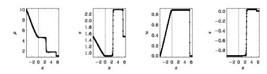
Figure 5: Standard shock tube test with an initial pressure jump of 1:10 and $\nu=0.6\delta x\,c_{\rm s}$ and $\chi/\nu=0.05$. The solid line indicates the analytic solution (in the limit $\tilde{\nu}\rightarrow 0$) and the dots the numerical solution. Note the small entropy excess on the right of the initial entropy discontinuity.

For stronger shocks velocity and entropy excess increase; see figures 6 and 7, where the initial pressure jumps are 1:100 and 1:1000, respectively, and the viscosities are chosen to be $\nu=1.6\delta x\,c_{\rm s}$ and $\nu=2.4\delta x\,c_{\rm s}$. (For the stationary shock problem considered below we also find that the viscosity must increase with the Mach number and, moreover, that the two should be proportional to each other.) In the cases shown in figures 6 and 7 we were able to put $\chi=0$ without getting any wiggles in $s$. However, in the case of strong shocks (pressure ratio 1:1000) the discrepancy between numerical and analytical solutions becomes quite noticeable.

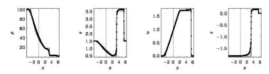
Figure 6: Same as figure 5, but for an initial pressure jump of 1:100 and $\nu=1.6\delta x\,c_{\rm s}$.

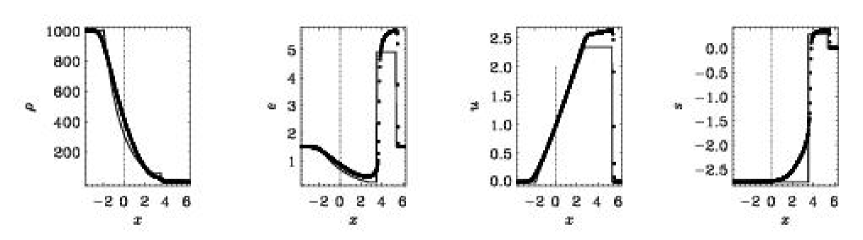
Figure 7: Same as figure 6, but for an initial pressure jump of 1:1000 and $\nu=2.4\delta x\,c_{\rm s}$.

In many practical applications shocks occur only in a small portion of space. One can therefore reduce the viscosity outside shocks or, conversely, use a small viscosity everywhere except in the locations of shock, i.e. where the flow is convergent (negative divergent). This leads to the concept of an artificial (Neumann-Richtmyer) shock viscosity,

$$\nu_{\rm shock}=c_{\rm shock}\delta x^{2}\,\langle(-\mbox{\boldmath$\nabla$}{}\cdot\mbox{\boldmath$u$}{})_{+}\rangle_{\rm n.n.},$$ (68)

where $\langle...\rangle_{\rm n.n.}$ indicates averaging over nearest neighbors and the subscript $+$ means that only the positive part is taken.

The last panel in figures 6 and 7 shows quite clearly how the entropy increases behind the shock. This entropy increase is just a consequence of the viscous heating term, $\tilde{\nu}u^{\prime 2}/h$. Without this term the solution would obviously be wrong everywhere behind the shock, especially when the shock is strong.

A somewhat simpler situation is encountered with standing shocks. In figure 8 we give an example of a numerically determined solution at Ma=100. The agreement in the jump for the numerically determined solution (dotted line and dots) and the theoretical solution (solid lines) is very good, although the position of the jump has moved away somewhat from the initial location ($x=0$), but this is merely a consequence of having used more-or-less arbitrarily a tanh profile to smooth the initial jumps. After some initial adjustment phase the profiles do indeed remain stationary. Note also, however, that the entropy profile is slightly shifted relative to the profiles of $u$ and $\Lambda$.

Figure 8: Example of a very strong standing shock with Ma=100. Note the relative shift of the position where $s$ increases relative to where $\Lambda=\ln\rho$ increases. The viscosity is chosen to be $\nu=\mbox{Ma}\times\delta x$.

It is interesting to note that when solving the Rankine-Hugionot jump conditions for shocks one is allowed to use the inviscid equations provided they are written in conservative form. Sometimes one finds in the literature the inviscid Navier-Stokes equations written in nonconservative form. This is not strictly correct, because without viscosity there would be no viscous heating and hence no entropy increase behind the shock. Moreover, it is quite common to consider a polytropic equation of state, $p=K\rho^{\Gamma}$. Again, in this case the entropy is constant, and so energy conservation is violated. Nevertheless, given that polytropic equations of state are often considered in astrophysics we consider this case in more detail in the next subsection.

3.6 Polytropic and isothermal shocks

For polytropes with $p=K\rho^{\Gamma}$, but $\Gamma\neq\gamma$ in general, we can write

$$-\mbox{\boldmath$\nabla$}{}h+h\mbox{\boldmath$\nabla$}{}s=-{1\over\rho}\mbox{\boldmath$\nabla$}{}p=-\mbox{\boldmath$\nabla$}{}\left({\Gamma K\over\Gamma-1}\rho^{\Gamma-1}\right)\equiv\mbox{\boldmath$\nabla$}{}\tilde{h},$$ (69)

so we can introduce a pseudo enthalpy $\tilde{h}$ as

$$\tilde{h}={\Gamma K\over\Gamma-1}\rho^{\Gamma-1}=\left[\left(1-{1\over\gamma}\right)\left/\left(1-{1\over\Gamma}\right)\right]\,h\right..$$ (70)

This is consistent with a fixed entropy dependence, where $s$ only depends on $\rho$ like

$$s=s(\rho)={1\over\gamma}\ln\left(p/\rho^{\gamma}\right)={1\over\gamma}\ln\left(K\,\rho^{\Gamma-\gamma}\right)={1\over\gamma}\ln K+\left({\Gamma\over\gamma}-1\right)\ln\rho,$$ (71)

which implies that in the polytropic case eq. (62) is discarded. In the adiabatic case, $\Gamma=\gamma$, entropy is constant. In the isothermal case, $p=c_{\rm s}^{2}\rho$, we have $\Gamma\rightarrow 1$, so entropy is not constant, but it varies only in direct relation to $-\ln\rho$ and not as a consequence of viscous heating behind the shock.

In deriving the Rankine-Hugionot jump conditions one uses the conservation of mass, momentum, and energy in a comoving frame, where the following three quantities are constants of motion:

$$J=\rho u,\quad I=\rho u^{2}+p,\quad E={\textstyle{1\over 2}}u^{2}+{\gamma\over\gamma-1}{p\over\rho}.$$ (72)

The values of these three constants can be calculated when all three variables, $u$, $p$, and $\rho$, are known on one side of the shock. For polytropic equations of state, with $p=K\rho^{\gamma}$, the energy equation is no longer used, so there are only the following two conserved quantities,

$$J=\rho u,\quad I=\rho u^{2}+K\rho^{\gamma}.$$ (73)

The dependence of the velocity, density, pressure, and entropy jumps on the upstream Mach number is plotted in figure 9 for the case $\gamma=5/3$ and compared with the polytropic case using $\Gamma=\gamma$.

Figure 9: The dependence of the velocity, density, pressure, and entropy jumps on the upstream Mach number for the case $\gamma=5/3$ (solid line) and comparison with the polytropic case using $\Gamma=\gamma$ (dotted line). Note that the velocity and density jumps saturate at 1/4 and 4, respectively, while there is no such saturation for the polytropic shock.

Figure 10: Like figure 9, but for $\gamma=\Gamma=1.0001$. Note that the velocity and density jumps saturate at much more extreme values than for $\gamma=5/3$. Thus, the results using polytropic and perfect gas equations agree up to much larger Mach numbers than for $\gamma=5/3$.

Note that the pressure jump, $p_{2}/p_{1}$, is almost independent of the value of $\gamma$ and does also not significantly depend on the polytropic assumption.

4 Nonuniform and lagrangian meshes

In many cases it is useful to consider nonuniform meshes, either by adding more points in places where large gradients are expected, or by letting the points move with the flow (lagrangian mesh). The lagrangian mesh is particularly useful in one-dimensional cases, because then the mesh topology (i.e. the ordering of mesh points) remains unchanged. Another method that gains constantly in popularity is adaptive mesh refinement (e.g., Grauer, Marliani, & Germaschewski 1998), which will not be discussed here.

4.1 Nonuniform topologically cartesian meshes

Nonuniform meshes can be implemented relative easily when each of the new coordinates depend on only one variable, for example when $x=x(\tilde{x})$, $y=y(\tilde{y})$, and $z=z(\tilde{z})$. Here, $\tilde{x}$, $\tilde{y}$ and $\tilde{z}$ are cartesian coordinates on a uniform mesh. In the more general case, however, we have

$$x=x(\tilde{x},\tilde{y},\tilde{z}),\quad y=y(\tilde{x},\tilde{y},\tilde{z}),\quad z=z(\tilde{x},\tilde{y},\tilde{z}),$$ (74)

so that $x$, $y$ and $z$ derivatives of a function $f$ can be calculated using the chain rule,

$${\partial f\over\partial x}={\partial f\over\partial\tilde{x}}{\partial\tilde{x}\over\partial x}+{\partial f\over\partial\tilde{y}}{\partial\tilde{y}\over\partial x}+{\partial f\over\partial\tilde{z}}{\partial\tilde{z}\over\partial x}\equiv{\partial f\over\partial\tilde{x}_{i}}{\partial\tilde{x}_{i}\over\partial x}.$$ (75)

Corresponding formulae apply obviously for the other two directions, so in general we can write

$${\partial f\over\partial x_{j}}={\partial f\over\partial\tilde{x}_{i}}J_{ij},\quad\mbox{where}\quad J_{ij}={\partial\tilde{x}_{i}\over\partial x_{j}}$$ (76)

is the jacobian of this coordinate transformation. This method allows one to have high resolution for example near a central object, without however having high resolution anywhere else far away from the central object. This is useful in connection with outflows from jets.

We discuss here one particular application that is relevant for simulating flows in a sphere. It is possible to transform a cartesian mesh to cover a sphere without a coordinate singularity. It will turn out, however, that there is a discontinuity in the jacobian. We discuss this here in 2-D. We denote the coordinate mesh by a tilde, so $(\tilde{x},\tilde{y})$ are the coordinates in a uniform cartesian mesh. We want to stretch the mesh such that points on the $\tilde{x}$ and $\tilde{y}$ axes are not affected, and that the distance of points on the diagonal is reduced by a factor $1/\sqrt{2}$ (or by $1/\sqrt{3}$ in 3-D). This can be accomplished by introducing new coordinates $(x,y)$ as

$$\pmatrix{x\cr y}=\pmatrix{\tilde{x}\cr\tilde{y}}\,{(\tilde{x}^{n}+\tilde{y}^{n})^{1/n}\over(\tilde{x}^{2}+\tilde{y}^{2})^{1/2}},$$ (77)

where $n$ is a large even number. In the limit $n\rightarrow\infty$ we may substitute

$$(\tilde{x}^{n}+\tilde{y}^{n})^{1/n}\rightarrow\max(|\tilde{x}|,|\tilde{y}|).$$ (78)

Examples of the resulting meshes for two different values of $n$ are given in figure 11.

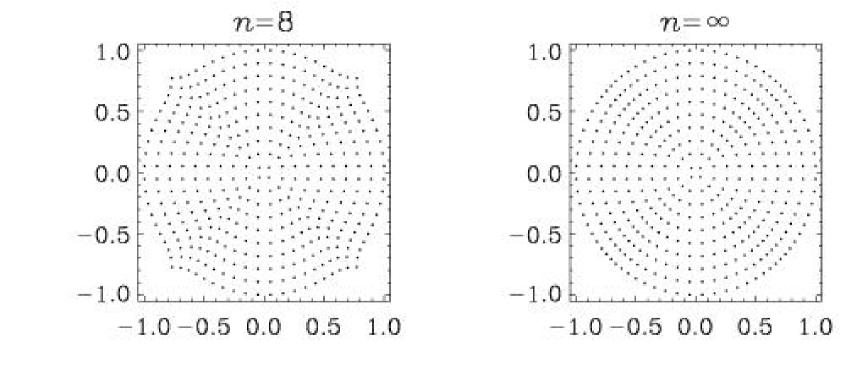
Figure 11: Examples of the resulting meshes for $n=8$ and $n\rightarrow\infty$ in which case eq. (78) is used.

In order to obtain the jacobian of this transformation, $\partial\tilde{x}_{i}/\partial x_{j}$, we have to consider separately the cases $\tilde{x}\geq\tilde{y}$ and $\tilde{x}\leq\tilde{y}$. The derivation is given in Appendix C, and is most concisely expressed in terms of the logarithmic derivative, so

$$\pmatrix{\displaystyle{\partial\ln\tilde{x}\over\partial\ln x}&\displaystyle{\partial\ln\tilde{x}\over\partial\ln y}\cr\displaystyle{\partial\ln\tilde{y}\over\partial\ln x}&\displaystyle{\partial\ln\tilde{y}\over\partial\ln y}}=\pmatrix{+1-\left(\displaystyle{\tilde{y}\over\tilde{r}}\right)^{2}&+1-\left(\displaystyle{\tilde{x}\over\tilde{r}}\right)^{2}\cr-1+\left(\displaystyle{\tilde{x}\over\tilde{r}}\right)^{2}&+1+\left(\displaystyle{\tilde{y}\over\tilde{r}}\right)^{2}}\quad\mbox{if $|\tilde{x}|\geq|\tilde{y}|$},$$ (79)

$$\pmatrix{\displaystyle{\partial\ln\tilde{x}\over\partial\ln x}&\displaystyle{\partial\ln\tilde{x}\over\partial\ln y}\cr\displaystyle{\partial\ln\tilde{y}\over\partial\ln x}&\displaystyle{\partial\ln\tilde{y}\over\partial\ln y}}=\pmatrix{+1+\left(\displaystyle{\tilde{x}\over\tilde{r}}\right)^{2}&-1+\left(\displaystyle{\tilde{y}\over\tilde{r}}\right)^{2}\cr+1-\left(\displaystyle{\tilde{y}\over\tilde{r}}\right)^{2}&+1-\left(\displaystyle{\tilde{x}\over\tilde{r}}\right)^{2}}\quad\mbox{if $|\tilde{x}|\leq|\tilde{y}|$},$$ (80)

where $\tilde{r}^{2}=\tilde{x}^{2}+\tilde{y}^{2}$. Note that the jacobian is discontinuous on the diagonals. This is a somewhat unfortunate feature of this transformation. It is not too surprising however that something like this happens, because the diagonals are the locations where a rotating flow must turn direction by $90^{\circ}$ in the coordinate mesh. Nevertheless, it is possible to obtain reasonably well behaved solutions; see figure 12 for an advection experiment using a prescribed differentially rotating flow.

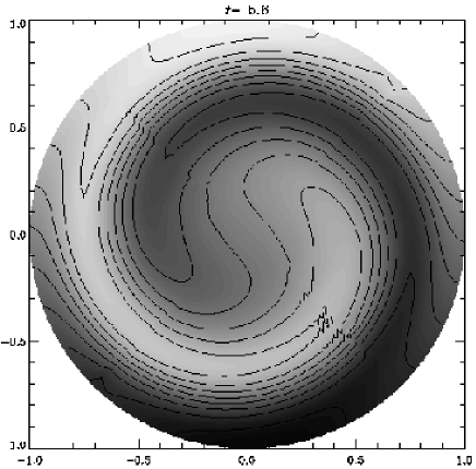
Figure 12: Example of an advection experiment on a $n=8$ mesh.

The fluid equations are still solved in rectangular cartesian coordinates, so for example the equation ${\rm D}{}s/{\rm D}{}t=0$ is solved in the form

$${\partial s\over\partial t}=-u_{x}{\partial s\over\partial x}-u_{y}{\partial s\over\partial y},$$ (81)

where the spatial derivatives are evaluated according to eq. (75). For the velocity field, stress-free boundary conditions, for example, would be written in the form

$$\hat{r}_{j}u_{j}=0,\quad\hat{\phi}_{i}S_{ij}\hat{r}_{j}=0,$$ (82)

where $S_{ij}$ is the rate of strain tensor, $\hat{r}_{j}$ and $\hat{\phi}_{i}$ are the cartesian components ($i=x,y,z$) of the radial and azimuthal unit vectors, i.e.

$$\hat{\mbox{\boldmath$r$}}{}={1\over r}\pmatrix{x\cr y},\quad\mbox{and}\quad\hat{\mbox{\boldmath$\phi$}}{}={1\over r}\pmatrix{-y\cr x}$$ (83)

are unit vectors in the $r$ and $\phi$ directions and $r=\sqrt{x^{2}+y^{2}}$ is the distance from the rotation axis. The stress-free boundary conditions are then

$$xu_{x}+yu_{y}=0$$ (84)

and

$$(x^{2}-y^{2})(u_{x,y}+u_{y,x})-2xy(u_{x,x}-u_{y,y})=0.$$ (85)

4.2 Lagrangian meshes

We now consider a simple one-dimensional lagrangian mesh problem. Assume that $\ell$ labels the particle, then the lagrangian derivative is

$${{\rm D}{}s\over{\rm D}{}t}\equiv\left({\partial s\over\partial t}\right)_{\ell={\rm const}}=\left({\partial s\over\partial t}\right)_{x={\rm const}}+\left({\partial x\over\partial t}\right)_{\ell={\rm const}}{\partial s\over\partial x}$$ (86)

Now, because

$$\left({\partial x\over\partial t}\right)_{\ell={\rm const}}={{\rm D}{}x\over{\rm D}{}t}=u$$ (87)

we have the well-known equation

$${{\rm D}{}s\over{\rm D}{}t}={\partial s\over\partial t}+u{\partial s\over\partial x}.$$ (88)

As an example we now consider the Burgers equation,

$${{\rm D}{}u\over{\rm D}{}t}=\tilde{\nu}{\partial^{2}u\over\partial x^{2}}.$$ (89)

We now take $u(x,t)=u(\ell(x),t)$ to be a function of the coordinate variable $\ell$ which, in turn, is a function of $x$. The $x$-derivatives are obtained using the chain rule, i.e.

$${\partial u\over\partial x}={\partial\ell\over\partial x}{\partial u\over\partial\ell}={u^{\prime}\over x^{\prime}},$$ (90)

and likewise for the second derivative

$${\partial^{2}u\over\partial x^{2}}={u^{\prime\prime}x^{\prime}-u^{\prime}x^{\prime\prime}\over x^{\prime 3}}.$$ (91)

Thus, the Burgers equation can then be written as $${\partial u\over\partial t}=\tilde{\nu}\,{u^{\prime\prime}x^{\prime}-u^{\prime}x^{\prime\prime}\over x^{\prime 3}},$$ (92) where the $x$ variable is given by $${\partial x\over\partial t}=u.$$ (93)

A solution of these two equations is given in figure 13.

Figure 13: Solution of the Burgers equation using a lagrangian mesh combined with a sixth order explicit scheme. The values of the mesh Reynolds number vary between $\delta x\,U/\nu=0.5$ and 2.0, where $\delta x$ refers to the initially uniform mesh spacing.

In the test problem above the initial meshpoint distribution was uniform. Although this is not quite suitable for this problem, it shows that subsequently the mesh spacing became narrower still, which means that the timestep in now governed by viscosity, $\delta t\leq 0.06\delta x^{2}_{\min}/\tilde{\nu}$, where the numerical factor is empirical. However, the mesh spacing does not need to be governed by eq. (93), so it is quite possible to come up with other prescriptions for the mesh spacing.

Consider as another example the isothermal eulerian equations

$${{\rm D}{}u\over{\rm D}{}t}=-c_{\rm s}^{2}{\partial\ln\rho\over\partial x}+\tilde{\nu}\left({\partial^{2}u\over\partial x^{2}}+{\partial\ln\rho\over\partial x}{\partial u\over\partial x}\right),$$ (94)

$${{\rm D}{}\ln\rho\over{\rm D}{}t}=-{\partial u\over\partial x}.$$ (95)

In lagrangian form they take the form

$${\partial u\over\partial t}=-c_{\rm s}^{2}{(\ln\rho)^{\prime}\over x^{\prime}}+\tilde{\nu}\,\left({u^{\prime\prime}x^{\prime}-u^{\prime}x^{\prime\prime}\over x^{\prime 3}}+{(\ln\rho)^{\prime}\over x^{\prime}}{u^{\prime}\over x^{\prime}}\right),$$ (96) $${\partial\ln\rho\over\partial t}=-{u^{\prime}\over x^{\prime}},$$ (97) $${\partial x\over\partial t}=u.$$ (98)

The example above demonstrates clearly the problem that lagrangian mesh points can continue to pile up near convergence points of the flow. This is a general problem with fully lagrangian schemes. One possible alternative is to use lagrangian-eulerian schemes (e.g., Benson 1992, Peterkin, Frese, & Sovinec 1998, Arber et al. 2001), which combine the advantages of lagrangian and eulerian codes, but involve obviously some kind of interpolation. Another alternative is to use a semi-lagrangian code which advects the mesh points not with the actual gas velocity $u$, but with a more independent mesh velocity $U$. Clearly, we want to avoid too small distances between neighboring points, so one could artificially lower the effective mesh velocity by involving for example the modulus of the jacobian, $|\mbox{\boldmath${\sf J}$}{}|$, which becomes large when the concentration of mesh points is high. Thus, one could choose for example $\mbox{\boldmath$U$}{}=\mbox{\boldmath$u$}{}/(1+|\mbox{\boldmath${\sf J}$}{}|)$. In the present case, $|\mbox{\boldmath${\sf J}$}{}|=|x^{\prime}|^{-1}$. In the following we discuss the formalism that needs to be invoked in order to calculate first and second derivatives on an advected mesh.

4.3 Non-lagrangian mesh advection

The main advantage of a lagrangian mesh is that it allows higher resolution locally. Another advantage, which is however less crucial, is that the nonlinear advection term drops out. The main disadvantage is however that a lagrangian mesh may become too distorted and overconcentrated, as seen in the previous section. In this subsection we address the possibility of advecting the mesh with a velocity $U$ that can be different from the fluid velocity. This way one can remove the swirl of the mesh by taking a velocity that is the gradient of some other quantity, i.e.

$$\mbox{\boldmath$U$}{}=-\mbox{\boldmath$\nabla$}{}\Phi_{\rm mesh},$$ (99)

where $\Phi_{\rm mesh}$ should be large in those regions where many points are needed. One possible criterion would be to require that the number of scale heights per meshpoint, $|\delta\mbox{\boldmath$x$}{}\cdot\mbox{\boldmath$\nabla$}{}\ln\rho|$, does not exceed an empirical value of $1/3$, say. Thus, $3|\delta\mbox{\boldmath$x$}{}\cdot\mbox{\boldmath$\nabla$}{}\ln\rho|<1$ would be a necessary condition. Another possibility would be to let $\Phi_{\rm mesh}$ evolve itself according to some suitable advection-diffusion equation. However, no generally satisfactory method seems to be available as yet. In order to calculate the jacobian for the coordinate transformation one can make use of the fact that the mesh evolves only gradually from one timestep to the next. For a more extended discussion of mesh advection schemes we refer to the article by Dorfi in the book by LeVeque et al. (1998).

4.3.1 Calculating the jacobian

Initially, at $t=0$, we have $\mbox{\boldmath$x$}{}=\tilde{\mbox{\boldmath$x$}{}}$. After the $n$th timestep, at $t=n\delta t$, we calculate the new $x$-mesh, $\mbox{\boldmath$x$}{}^{(n+1)}$, from the previous one, $\mbox{\boldmath$x$}{}^{(n)}$, i.e.

$$\mbox{\boldmath$x$}{}^{(n+1)}=\mbox{\boldmath$x$}{}^{(n)}+\mbox{$\mbox{\boldmath$U$}{}\left(\mbox{\boldmath$x$}{}^{(n)},t\right)\,\delta t$}.$$ (100)

Here, $\mbox{\boldmath$x$}{}^{(0)}=\tilde{\mbox{\boldmath$x$}{}}$ is just the original coordinate mesh. Differentiating the $i$th component with respect to the $j$th component, as we have done in § 4.1, we obtain

$$\delta_{ij}={\partial x^{(n+1)}_{i}\over\partial x^{(n+1)}_{j}}={\partial x^{(n)}_{i}\over\partial x^{(n+1)}_{j}}+{\partial U^{(n)}_{i}\over\partial x^{(n+1)}_{j}}\,\delta t,$$ (101)

where $U^{(n)}_{i}=U_{i}\left(\mbox{\boldmath$x$}{}^{(n)},t\right)$. In the expression above we have $U_{i}$ on the mesh $\mbox{\boldmath$x$}{}^{(n)}$, but we need to differentiate with respect to the new mesh $\mbox{\boldmath$x$}{}^{(n+1)}$. This can be fixed by another factor $\partial x^{(n)}_{i}/\partial x^{(n+1)}_{j}$. Thus, we have

$$\delta_{ij}={\partial x^{(n)}_{i}\over\partial x^{(n+1)}_{j}}+{\partial x^{(n)}_{k}\over\partial x^{(n+1)}_{j}}{\partial U_{i}\left(\mbox{\boldmath$x$}{}^{(n)},t\right)\over\partial x^{(n)}_{k}}\,\delta t=\left[\delta_{ik}+{\partial U^{(n)}_{i}\over\partial x^{(n)}_{k}}\,\delta t\right]{\partial x^{(n)}_{k}\over\partial x^{(n+1)}_{j}}.$$ (102)

This can be written in matrix form,

$$\delta_{ij}={\sf M}_{ik}{\sf J}^{(n)}_{kj},$$ (103)

where

$${\sf M}_{ik}=\delta_{ik}+{\partial U_{i}\left(\mbox{\boldmath$x$}{}^{(n)},t\right)\over\partial x^{(n)}_{k}}\,\delta t$$ (104)

is a transformation matrix and

$${\sf J}^{(n)}_{ij}={\partial x^{(n)}_{i}\over\partial x^{(n+1)}_{j}}$$ (105)

is the incremental jacobian, so $\mbox{\boldmath${\sf J}$}{}^{(n)}=\mbox{\boldmath${\sf M}$}{}^{-1}$. To obtain the jacobian at $t=2\delta t$, for example, we calculate

$${\partial x^{(0)}_{i}\over\partial x^{(2)}_{j}}={\partial x^{(0)}_{i}\over\partial x^{(1)}_{k}}{\partial x^{(1)}_{k}\over\partial x^{(2)}_{j}}={\sf J}^{(0)}_{ik}{\sf J}^{(1)}_{kj}\equiv\left(\mbox{\boldmath${\sf J}$}{}^{(0)}\mbox{\boldmath${\sf J}$}{}^{(1)}\right)_{ij}.$$ (106)

The jacobian at $t=n\delta t$ is then obtained by successive matrix multiplication from the right, so

$${\sf J}_{ij}^{\rm(0\rightarrow n+1)}={\sf J}_{ik}^{\rm(0\rightarrow n)}{\sf J}_{kj}^{(n)},$$ (107)

where ${\sf J}_{ij}^{\rm(0\rightarrow n+1)}$ and ${\sf J}_{ij}^{\rm(0\rightarrow n)}$ are the full (as opposed to incremental) jacobians at the new and previous timesteps, respectively.

4.3.2 Calculating the second order jacobian

A corresponding calculation (see Appendix D) for the second derivatives of a function $f$ shows that

$${\partial^{2}f\over\partial x_{i}\partial x_{j}}={\partial^{2}f\over\partial\tilde{x}_{p}\partial\tilde{x}_{q}}{\sf J}_{pi}{\sf J}_{qj}+{\partial f\over\partial\tilde{x}_{k}}{\sf K}_{kij},$$ (108)

where

$${\sf K}_{kij}={\partial^{2}\tilde{x}_{k}\over\partial x_{i}\partial x_{j}}$$ (109)

is the second order jacobian. Like for the first derivative the second order jacobian can be obtained by successive tensor multiplication,

$${\sf K}_{kij}^{\rm(0\rightarrow n+1)}={\sf K}_{kpq}^{\rm(0\rightarrow n)}{\sf J}_{pi}^{(n)}{\sf J}_{qj}^{(n)}+{\sf J}_{kl}^{\rm(0\rightarrow n)}{\sf K}_{lij}^{(n)},$$ (110)

where ${\sf K}_{kij}^{\rm(0\rightarrow n+1)}$ and ${\sf K}_{kij}^{\rm(0\rightarrow n)}$ are the second order jacobians at the new and previous timesteps, respectively, and

$${\sf K}^{(n)}_{kij}={\partial^{2}x^{(n)}_{k}\over\partial x^{(n+1)}_{i}\partial x^{(n+1)}_{j}}$$ (111)

is the incremental second order jacobian, which is calculated at each timestep as

$${\sf K}^{(n)}_{kij}=-\delta t\left(\mbox{\boldmath${\sf M}$}{}^{-1}\right)_{kl}\,U_{l,pq}{\sf J}_{pi}^{(n)}{\sf J}_{qj}^{(n)},$$ (112)

where ${\sf M}$ was defined in eq. (104) and

$$U_{l,pq}={\partial^{2}U_{l}\left(\mbox{\boldmath$x$}{}^{(n)},t\right)\over\partial x^{(n)}_{p}\partial x^{(n)}_{q}}$$ (113)

is the second order velocity gradient matrix on the physical mesh. Since $\mbox{\boldmath${\sf M}$}{}^{-1}=\mbox{\boldmath${\sf J}$}{}^{(n)}$ is just the incremental jacobian, we can write (112) as

$${\sf K}^{(n)}_{kij}=-{\sf J}_{kl}^{(n)}\delta t\,U_{l,pq}{\sf J}_{pi}^{(n)}{\sf J}_{qj}^{(n)}.$$ (114)

Since the expressions (110) and (114) involve both a multiplication with ${\sf J}_{pi}^{(n)}{\sf J}_{qj}^{(n)}$, we can simplify eq. (110) to give

$${\sf K}_{kij}^{\rm(0\rightarrow n+1)}=\left[{\sf K}_{kpq}^{\rm(0\rightarrow n)}-{\sf J}_{kl}^{\rm(0\rightarrow n)}{\sf J}_{lm}^{(n)}\delta t\,U_{m,pq}\right]{\sf J}_{pi}^{(n)}{\sf J}_{qj}^{(n)}.$$ (115)

Here the expression ${\sf J}_{kl}^{\rm(0\rightarrow n)}{\sf J}_{lm}^{(n)}$ is of course the new jacobian, ${\sf J}_{kl}^{\rm(0\rightarrow n+1)}$.

So in summary, the new first and second order jacobians are obtained from the previous ones via the formulae $${\sf J}_{ij}^{\rm(0\rightarrow n+1)}={\sf J}_{ik}^{\rm(0\rightarrow n)}{\sf J}_{kj}^{(n)},$$ (116) $${\sf K}_{kij}^{\rm(0\rightarrow n+1)}=\left[{\sf K}_{kpq}^{\rm(0\rightarrow n)}-{\sf J}_{kl}^{\rm(0\rightarrow n+1)}\delta t\,U_{l,pq}\right]{\sf J}_{pi}^{(n)}{\sf J}_{qj}^{(n)},$$ (117) $${\partial f\over\partial x_{i}}={\partial f\over\partial\tilde{x}_{p}}{\sf J}_{pi},$$ (118) $${\partial^{2}f\over\partial x_{i}\partial x_{j}}={\partial^{2}f\over\partial\tilde{x}_{p}\partial\tilde{x}_{q}}{\sf J}_{pi}{\sf J}_{qj}+{\partial f\over\partial\tilde{x}_{k}}{\sf K}_{kij},$$ (119) where $\mbox{\boldmath${\sf J}$}{}\equiv\mbox{\boldmath${\sf J}$}{}^{\rm(0\rightarrow n+1)}$ and $\mbox{\boldmath${\sf K}$}{}\equiv\mbox{\boldmath${\sf K}$}{}^{\rm(0\rightarrow n+1)}$ has been assumed.

Since now the mesh is moving in time with the local speed $U$ which is different from the gas velocity $u$, the lagrangian derivative is

$${{\rm D}{}\over{\rm D}{}t}={\partial\over\partial t}+(\mbox{\boldmath$u$}{}-\mbox{\boldmath$U$}{})\cdot\mbox{\boldmath$\nabla$}{}.$$ (120)

In all other respects the basic equations, written in cartesian form, are still unchanged, provided all $x$, $y$, and $z$ derivatives (first and second) are evaluated, as in (75) and (108), with the components of the jacobian. As an example we show in figure 14 the result of a kinematic collapse calculation where ${\rm D}{}\mbox{\boldmath$u$}{}/{\rm D}{}t=-\mbox{\boldmath$\nabla$}{}\phi$ and ${\rm D}{}s/{\rm D}{}t=0$ with a smoothed but localized gravitational potential $\phi$. In figure 15 we compare the results of an eulerian and a lagrangian calculation using the same number of meshpoints. Already after some short time the eulerian calculation begins to become underresolved and develops wiggles while the lagrangian calculation proceeds without problems.

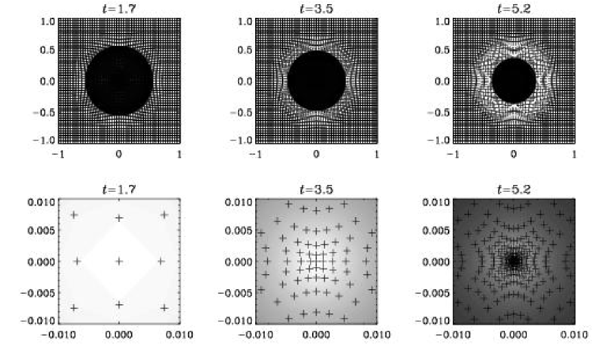
Figure 14: Example of a collapse calculation. The second row shows only the inner parts with $|x|,\,|y|\leq 0.01$ at the same times as in the upper row.

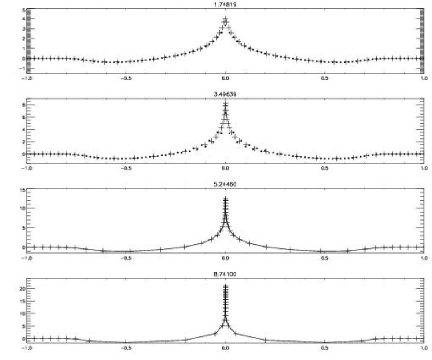
Figure 15: Comparison of lagrangian (+ signs) and eulerian (dots) calculations in the first two plots, and later development (last two plots) where the eulerian no longer works. Note that already in the second plot the eulerian calculation has developed noticeable wiggles which the lagrangian proceeds without problems.

4.4 Unstructured meshes

We now discuss how we can calculate spatial derivatives of our variables from a nonuniformly spaced ensemble of points. Consider the function $f(x,y,z)$, which stand for one of the components of a vector (velocity or magnetic vector potential) or a scalar, such as $\ln\rho$. We approximate the function $f(x,y,z)$ in the neighborhood of the point $\mbox{\boldmath$x$}{}_{i}=(x_{i},y_{i},z_{i})$ by a multidimensional polynomial of degree $N$,

$$f(x,y,z)=f(x_{i},y_{i},z_{i})+\sum_{l+m+n\leq N}c_{lmn}(x-x_{i})^{l}(y-y_{i})^{m}(z-z_{i})^{n},$$ (121)

where $l$, $m$, and $n$ are non-negative integers and $c_{lmn}$ are coefficients that are to be determined separately for each point by applying eq. (121) to all neighboring points $\mbox{\boldmath$x$}{}_{j}$. Note that $c_{000}=0$ and does not need to be considered. Thus, for each point $j$ we have a system of equations

$$f_{ij}=\sum_{l+m+n\leq N}{1\over l!\,m!\,n!}c_{lmn}x_{ij}^{l}\,y_{ij}^{m}\,z_{ij}^{n},$$ (122)

where $f_{ij}=f(x_{i},y_{i},z_{i})-f(x_{j},y_{j},z_{j})$ and $\mbox{\boldmath$x$}{}_{ij}=\mbox{\boldmath$x$}{}_{i}-\mbox{\boldmath$x$}{}_{j}$. This system of equations can be written in matrix form

$$f_{\alpha}={\sf M}_{\alpha\beta}C_{\beta},$$ (123)

where $1\leq(\alpha,\beta)\leq M$ and $M$ is the spatial dimension of the matrix, which is related to $N$ and the dimension as follows:

$$M=\left\{\begin{array}[]{ll}N&\mbox{in 1-D},\\ (N+1)(N+2)/2-1&\mbox{in 2-D},\\ (N+1)(3N/2)&\mbox{in 3-D}.\end{array}\right.$$ (124)

When $N=2$ the matrix ${\sf M}$ is given by

$$\mbox{\boldmath${\sf M}$}{}=\pmatrix{x_{ij_{1}}&y_{ij_{1}}&z_{ij_{1}}&{\textstyle{1\over 2}}x_{ij_{1}}^{2}&x_{ij_{1}}y_{ij_{1}}&{\textstyle{1\over 2}}y_{ij_{1}}^{2}&y_{ij_{1}}z_{ij_{1}}&{\textstyle{1\over 2}}z_{ij_{1}}^{2}&z_{ij_{1}}x_{ij_{1}}\cr x_{ij_{2}}&y_{ij_{2}}&z_{ij_{2}}&{\textstyle{1\over 2}}x_{ij_{2}}^{2}&x_{ij_{2}}y_{ij_{2}}&{\textstyle{1\over 2}}y_{ij_{2}}^{2}&y_{ij_{2}}z_{ij_{2}}&{\textstyle{1\over 2}}z_{ij_{2}}^{2}&z_{ij_{2}}x_{ij_{2}}\cr...&...&...&...&...&...&...&...&...\cr x_{ij_{M}}&y_{ij_{M}}&z_{ij_{M}}&{\textstyle{1\over 2}}x_{ij_{M}}^{2}&x_{ij_{M}}y_{ij_{M}}&{\textstyle{1\over 2}}y_{ij_{M}}^{2}&y_{ij_{M}}z_{ij_{M}}&{\textstyle{1\over 2}}z_{ij_{M}}^{2}&z_{ij_{M}}x_{ij_{M}}}$$ (125)

and

$$\mbox{\boldmath$C$}{}=\left(c_{100},c_{010},c_{001},c_{200},c_{110},c_{020},c_{011},c_{002},c_{101}\right)^{T}.$$ (126)

Here, $j_{n}$ ($n=1,2,...,M$) are the $M$ nearest neighbors of the point $i$. In general the matrix can be written in the form

$$M_{\alpha\beta}^{(J)}=x_{\alpha J}^{l(\beta)}y_{\alpha J}^{m(\beta)}z_{\alpha J}^{n(\beta)},$$ (127)

where $J$ is the index of the point at which the derivative is to be calculated. The set of exponents $l(\beta)$, $m(\beta)$, and $n(\beta)$ is given here for the case $N=4$ in 3-D:

$$l(\beta)=(1,0,0|2,1,0,0,0,1|3,2,1,0,0,0,0,1,2|4,3,2,1,0,0,0,0,0,1,2,3),$$ (128)

$$m(\beta)=(0,1,0|0,1,2,1,0,0|0,1,2,3,2,1,0,0,0|0,1,2,3,4,3,2,1,0,0,0,0),$$ (129)

$$n(\beta)=(0,0,1|0,0,0,1,2,1|0,0,0,0,1,2,3,2,1|0,0,0,0,0,1,2,3,4,3,2,1),$$ (130)

where the vertical bars separate the sets of exponents that correspond to increasing orders. Once the $C$ vector has been obtained, the first derivatives of $f$ are simply given by

$${\partial f\over\partial x}=c_{100},\quad{\partial f\over\partial y}=c_{010},\quad{\partial f\over\partial z}=c_{001}.$$ (131)

Likewise, the second derivatives are given by

$${\partial^{2}f\over\partial x^{2}}=c_{200},\quad{\partial^{2}f\over\partial y^{2}}=c_{020},\quad{\partial^{2}f\over\partial z^{2}}=c_{002},$$ (132)

and the mixed second derivatives are given by

$${\partial^{2}f\over\partial x\partial y}=c_{110},\quad{\partial^{2}f\over\partial y\partial z}=c_{011},\quad{\partial^{2}f\over\partial z\partial x}=c_{101}.$$ (133)

Although this method can be used for meshes that are static in time, it can also be used in connection with multi-dimensional lagrangian schemes. In that case there may arise the problem that neighboring points get very close together, and so small errors strongly affect the coefficients. A good way out of this is to use a few more points and to solve the linear matrix equation using singular value decomposition. An example of such a calculation is shown in figure 16, where a passive scalar, with the initial distribution $A(\mbox{\boldmath$x$}{},0)=x$, is advected by the velocity, $\mbox{\boldmath$u$}{}=\dot{\mbox{\boldmath$r$}{}}$, which in turn is obtained by solving Kepler’s equation, $\ddot{\mbox{\boldmath$r$}{}}=-GM\mbox{\boldmath$r$}{}/r^{3}$, using the normalization $GM=1$. This windup problem corresponds to the windup of initially horizontal magnetic field lines.

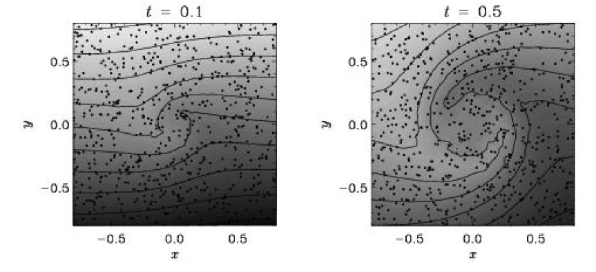
Figure 16: Two-dimensional advection problem on an unstructured lagrangian mesh. The dots indicate the 1000 lagrangian particles which constitute the unstructured mesh.

In diffusivity used in figure 16 was $\eta=0.02$, but due to the coarse resolution and the implicit smoothing resulting from the singular value decomposition technique the effective diffusivity is somewhat larger.

5 Implementing magnetic fields

As mentioned in § 2, implementing magnetic fields is relatively straightforward. On the one hand, the magnetic field causes a Lorentz force, $\mbox{\boldmath$J$}{}\times\mbox{\boldmath$B$}{}$, where $B$ is the flux density, $\mbox{\boldmath$J$}{}=\mbox{\boldmath$\nabla$}{}\times\mbox{\boldmath$B$}{}/\mu_{0}$ is the current density, and $\mu_{0}$ is the vacuum permeability. Note, however, that $\mbox{\boldmath$J$}{}\times\mbox{\boldmath$B$}{}$ is the force per unit volume, so in eq. (9) we need to add the term $\mbox{\boldmath$J$}{}\times\mbox{\boldmath$B$}{}/\rho$ on the right hand side. On the other hand, $B$ itself evolves according to the Faraday equation,

$${\partial\mbox{\boldmath$B$}{}\over\partial t}=-\mbox{\boldmath$\nabla$}{}\times\mbox{\boldmath$E$}{}$$ (134)

where the electric field $E$ can be expressed in terms of $J$ using Ohm’s law in the laboratory frame, $\mbox{\boldmath$E$}{}=-\mbox{\boldmath$u$}{}\times\mbox{\boldmath$B$}{}+\mbox{\boldmath$J$}{}/\sigma$, where $\sigma=(\eta\mu_{0})^{-1}$ is the electric conductivity and $\eta$ is the magnetic diffusivity.

In addition we have to satisfy the condition $\mbox{\boldmath$\nabla$}{}\cdot\mbox{\boldmath$B$}{}=0$. This is most easily done by solving not for $B$, but instead for the magnetic vector potential $A$, where $\mbox{\boldmath$B$}{}=\mbox{\boldmath$\nabla$}{}\times\mbox{\boldmath$A$}{}$. The evolution of $A$ is governed by the uncurled form of eq. (134),

$${\partial\mbox{\boldmath$A$}{}\over\partial t}=-\mbox{\boldmath$E$}{}-\mbox{\boldmath$\nabla$}{}\phi$$ (135)

where $\phi$ is the electrostatic potential, which takes the role of an integration constant which does not affect the evolution of $B$. The choice $\phi=0$ is most advantageous on numerical grounds. (By contrast, the Coulomb gauge $\nabla\cdot\mbox{\boldmath$A$}{}=0$, which is very popular in analytic considerations, would obviously be of no advantages, since one still has the problem of solving a the solenoidality condition.

Solving for $A$ instead of $B$ has significant advantages, even though this involves taking another derivative. However, the total number of derivatives taken in the code is essentially the same. In fact, when centered finite differences are employed, Alfvén waves are better resolved when $A$ is used, because then the system of equations for one-dimensional Alfvén waves in the presence of a uniform $B_{x0}$ field in a medium of constant density $\rho_{0}$ reduces to

$$\dot{u}_{z}={1\over\mu_{0}\rho_{0}}B_{x0}A_{y}^{\prime\prime},\quad\dot{A}_{y}=B_{x0}u_{z},$$ (136)

where a second derivative is taken only once (primes denote $x$-derivatives). If, instead, one solves for the $B_{z}$ field, one has

$$\dot{u}_{z}={1\over\mu_{0}\rho_{0}}B_{x0}B_{z}^{\prime},\quad\dot{B}_{z}=B_{x0}u_{z}^{\prime},$$ (137)

where a first derivative is applied twice, which is far less accurate at small scales if a centered finite difference scheme is used. At the Nyquist frequency, for example, the first derivative is zero and applying an additional first derivative gives still zero. By contrast, taking a second derivative once gives of course not zero. The use of a staggered mesh circumvents this difficulty. However, such an approach introduces additional complications which hamper the ease with which the code can be adapted to other problems.

Another advantage of using $A$ is that it is straightforward to evaluate the magnetic helicity, $\langle\mbox{\boldmath$A$}{}\cdot\mbox{\boldmath$B$}{}\rangle$, which is a particularly important quantity to monitor in connection with dynamo and reconnection problems.

The main advantage of solving for $A$ is of course that one does not need to worry about the solenoidality of the $B$-field, even though one may want to employ irregular meshes or complicated boundary conditions.

As we have emphasized before, when centered meshes are used, it is usually a good idea to avoid taking first derivatives of the same variable twice, because it is more accurate to take instead a second derivative only once. For this reason we calculate the current not as $\mbox{\boldmath$J$}{}=\mu_{0}^{-1}\mbox{\boldmath$\nabla$}{}\times(\mbox{\boldmath$\nabla$}{}\times\mbox{\boldmath$A$}{})$, but as

$$\mbox{\boldmath$J$}{}=\mu_{0}^{-1}\left[-\nabla^{2}\mbox{\boldmath$A$}{}+\mbox{\boldmath$\nabla$}{}(\mbox{\boldmath$\nabla$}{}\cdot\mbox{\boldmath$A$}{})\right].$$ (138)

Taking the gradient of $\mbox{\boldmath$\nabla$}{}\cdot\mbox{\boldmath$A$}{}$ involves of course also taking first derivatives of the same variable twice, but these contributions are canceled by corresponding components of the $\nabla^{2}\mbox{\boldmath$A$}{}$ term. There are some advantages relying here on the numerical cancellation, which is of course not exact. The reason is that the full $\nabla^{2}\mbox{\boldmath$A$}{}$ term is important when used in the magnetic diffusion term. If the diagonal terms, $\partial^{2}A_{x}/\partial x^{2}$, $\partial^{2}A_{y}/\partial y^{2}$, and $\partial^{2}A_{z}/\partial z^{2}$, which would all drop out analytically, were taken out there would be no diffusion of $A$ in the direction of $A$.

There is one more aspect that is often useful keeping in mind. There is a particular gauge that allows one to rewrite the uncurled induction equation in such a form that the evolution of $A$ is controlled by the advective derivative of $A$. The calculation is easy. Write the induction term $\mbox{\boldmath$u$}{}\times\mbox{\boldmath$B$}{}$ in component form and express $B$ in terms of $A$, so

$$(\mbox{\boldmath$u$}{}\times\mbox{\boldmath$\nabla$}{}\times\mbox{\boldmath$A$}{})_{i}=u_{j}(\partial_{i}A_{j}-\partial_{j}A_{i})=\partial_{i}(u_{j}A_{j})-A_{j}\partial_{i}u_{j}-u_{j}\partial_{j}A_{i}.$$ (139)

Here the last term contributes to the advective derivative, the first term can be removed by a gauge transformation and the middle term is a modified stretching term, so the induction equation takes the form

$${{\rm D}{}A_{i}\over{\rm D}{}t}=-A_{j}\partial_{i}u_{j}-\eta\mu_{0}J_{i}.$$ (140)

This gauge was used by Brandenburg et al. (1995) in order to treat a linear velocity shear using pseudo-periodic (shearing box) boundary conditions. The formulation (140) can also be useful when solving the induction equation using lagrangian methods. Note, however, that the nonresistive evolution of $A$ differs from that of $B$ in that the indices of the matrix ${\sf U}_{ij}\equiv\partial u_{i}/\partial x_{j}$ are interchanged and that the sign is different; positive for the $B$-equation,

$${{\rm D}{}B_{i}\over{\rm D}{}t}=+{\sf U}_{ij}B_{j}+\mbox{other terms},$$ (141)

and negative for the $A$-equation,

$${{\rm D}{}A_{i}\over{\rm D}{}t}=-A_{j}{\sf U}_{ji}+\mbox{other terms}.$$ (142)

These two formulations are particularly advantageous when the velocity has a constant gradient, as in the case of linear shear. In local simulations of accretion discs, for example, the shear component is $u_{y}(x)=-{3\over 2}\Omega x$, so ${\sf U}_{yx}=-{3\over 2}\Omega$, and all other ${\sf U}_{ij}$ vanish. Hence

$${{\rm D}{}A_{x}\over{\rm D}{}t}=+{3\over 2}\Omega A_{y}+\mbox{other terms}$$ (143)

for the $A$-formulation, or

$${{\rm D}{}B_{y}\over{\rm D}{}t}=-{3\over 2}\Omega B_{x}+\mbox{other terms}$$ (144)

for the $B$-formulation. In these two formulations all dependent variables are clearly periodic (or rather pseudo-periodic), so there is no term that is explicitly non-periodic such as $u_{y}(x)=-{3\over 2}\Omega x$. In the following, whenever magnetic fields are present, we use the $A$-formulation, mainly because it guarantees the solenoidality of $B$ everywhere (including the boundaries), and also because it is easy to use.

Cache-efficient coding

Unlike the CRAY computers that dominated supercomputing in the 80ties and early 90ties, all modern computers have a cache that constitutes a significant bottleneck for many codes. This is the case if large three-dimensional arrays are constantly used within each time step. The advantage of this way of coding is clearly the conceptual simplicity of the code. A more cache-efficient way of coding is to calculate an entire timestep (or a corresponding substep in a three-stage $2N$ Runge-Kutta scheme) only along a one-dimensional pencil of data within the box. On Linux and Irix architectures, for example, this leads to a speed-up by 60%. An additional advantage is a drastic reduction in temporary storage that is needed for auxiliary variables within each time step.

6 Application to astrophysical outflows

6.1 The isothermal Parker wind

Before discussing outflows from accretion discs it is illuminating to consider first the one-dimensional example of pressure-driven outflows in spherical geometry. A particularly simple case is the isothermal wind problem, which is governed by the equations

$${\partial u\over\partial t}+u{\partial u\over\partial r}=-c_{\rm s}^{2}{\partial\ln\rho\over\partial r}-{\partial\Phi\over\partial r},$$ (145)

$${\partial\ln\rho\over\partial t}+u{\partial\ln\rho\over\partial r}=-{1\over r^{2}}{\partial\over\partial r}(r^{2}u)+{\dot{M}\xi(r)\over\rho},$$ (146)

where $c_{\rm s}$ is the isothermal sound speed (assumed constant), $\dot{M}$ is the mass loss rate, and $\xi(r)$ is a prescribed function of position, normalized such that $\int 4\pi r^{2}\xi(r){\rm d}{}r=1$, and non-vanishing only near $r=0$. For a point mass the gravity potential $\Phi$ would be $-GM/r$, but this becomes singular at the origin. Therefore we use the expression $\Phi=-GM/(r^{n}+r_{0}^{n})^{1/n}$ instead, where we choose $n=5$ in all cases, and $1/r_{0}$ gives the depth of the potential well. In figure 17 we show radial velocity and density profiles for different values of $\dot{M}$. Note that the velocity profile is independent of the value of $\dot{M}$, but the density profile changes by a constant factor. In the steady case the equations can be combined to

$$\left(u^{2}-c_{\rm s}^{2}\right){{\rm d}{}\ln|u|\over{\rm d}{}r}={2c_{\rm s}^{2}\over r}-{GM\over r^{2}},$$ (147)

so the sonic point, $|u|=c_{\rm s}$, is at $r=r_{*}=GM/2c_{\rm s}^{2}$. In figure 17 we have chosen $GM=2$ and $c_{\rm s}=1$, so $r_{*}=1$, which is consistent with the graph of $u$.

Figure 17: Isothermal Parker wind solutions for different values of $\dot{M}$. Note that the $u$ profile is independent of the value of $\dot{M}$. $GM=2$, $c_{\rm s}=1$, $r_{0}=0.4$.

6.2 The polytropic or adiabatic wind

In the following we make the assumption that the entropy is constant. In that case it is particularly useful to solve for the potential enthalpy, $H\equiv h+\Phi$, which varies much less than either $h$ or $\Phi$. Using $H$ as dependent variable is particularly useful if one solves the equations all the way to the origin, $r=0$, where $\Phi$ tends to become singular (or at least strongly negative if a smoothed potential is used). In terms of $H$ the governing equations are

$${\partial u\over\partial t}+u{\partial u\over\partial r}=-{\partial H\over\partial r}-u\dot{M}\xi,$$ (148)

$${\partial H\over\partial t}+u{\partial H\over\partial r}=u{\partial\Phi\over\partial r}+c_{\rm s}^{2}\left[-{1\over r^{2}}{\partial\over\partial r}(r^{2}u)+{\dot{M}\xi(r)\over\rho}\right],$$ (149)

where $H=h+\Phi$ is the potential enthalpy, $h=p/\rho+e$ is the enthalpy, and $c_{\rm s}^{2}=(\gamma-1)h=(\gamma-1)(H-\Phi)$ for a perfect gas, where $c_{\rm s}$ is the adiabatic sound speed and $h=c_{p}T$ is the enthalpy. These equations are also valid in the nonisothermal case ($\gamma\neq 1$). The isothermal case may be recovered by putting $\gamma=1$ and replacing $h$ by $c_{\rm s}^{2}\ln\rho$. In figure 18 we show solutions for different values of $\dot{M}$ and $\gamma=5/3$. Again we put $GM=2$ and $c_{\rm s0}=1$.

Figure 18: Polytropic Parker wind solutions for different values of $\dot{M}$. $GM=2$, $c_{\rm s0}=1$, $r_{0}=0.4$.

We note that, depending on the strength of the mass source, the polytropic wind problem allows a variety of different velocity and Mach number profiles, whereas for the isothermal wind problem there was only one solution possible, independent of the strength of the mass source. The velocity profile was always the same and also the density was the same up to some scaling factor that changes with $\dot{M}$. This is connected with the additional degree of freedom introduced through the polytropic constant $K=p/rho^{\gamma}$. Since $c_{\rm s}$ is no longer constant, the position of the sonic point is no longer fixed and different solutions are possible.

In figure 19 we show solutions where $\dot{M}$ is kept constant, but the depth of the potential well, $GM/r_{0}$, is changed by varying the value of $r_{0}$. Note that the deeper the potential well, the higher the wind speed. The density far away from the source is then correspondingly smaller, so as to maintain the same mass flux.

Figure 19: Density $\rho$, velocity $u$, and Mach number $\mbox{Ma}=u/c_{\rm s}$ for the polytropic Parker wind solutions for different values of $r_{0}$. $GM=2$, $c_{\rm s0}=1$, $\dot{M}=10$.

As we have seen in § 3.6, a polytropic equation of state is unphysical. Therefore we now consider the case where the energy equation is included. To be somewhat more general we consider first the basic equations in conservative form with mass, momentum and energy sources included, i.e.

$${\partial\rho\over\partial t}+{\partial\over\partial x_{j}}\left(\rho u_{j}\right)=\dot{M}\xi,$$ (150)

$${\partial\over\partial t}\left(\rho u_{i}\right)+{\partial\over\partial x_{j}}\left(\rho u_{i}u_{j}+p\delta_{ij}-\tau_{ij}\right)=\dot{I}_{i}\xi,$$ (151)

$${\partial\over\partial t}\left({\textstyle{1\over 2}}\rho\mbox{\boldmath$u$}{}^{2}+\rho e\right)+{\partial\over\partial x_{j}}\left[u_{j}\left({\textstyle{1\over 2}}\rho\mbox{\boldmath$u$}{}^{2}+\rho h\right)-u_{i}\tau_{ij}\right]=\dot{E}\xi,$$ (152)

where $\dot{M}$, $\dot{\mbox{\boldmath$I$}{}}$, and $\dot{E}$ are the rates of mass, momentum and energy injection into the system, $\tau_{ij}=2\nu\rho{\sf S}_{ij}$ is the viscous stress tensor, and ${\sf S}_{ij}$ is the (traceless) rate of strain tensor; see eq. (12). Rewriting the energy equation in nonconservative form we have

$${{\rm D}{}e\over{\rm D}{}t}+{p\over\rho}\mbox{\boldmath$\nabla$}{}\cdot\mbox{\boldmath$u$}{}\equiv T{{\rm D}{}s\over{\rm D}{}t}=2\nu\mbox{\boldmath${\sf S}$}{}^{2}+\left[\dot{E}-\mbox{\boldmath$u$}{}\cdot\left(\dot{\mbox{\boldmath$I$}{}}-\mbox{\boldmath$u$}{}\dot{M}\right)-\left({\textstyle{1\over 2}}\mbox{\boldmath$u$}{}^{2}+e\right)\dot{M}\right]{\xi(r)\over\rho},$$ (153)

which can also be rewritten in terms of entropy, so the final system of nonconservative equations with source terms is

$${{\rm D}{}\ln\rho\over{\rm D}{}t}+\mbox{\boldmath$\nabla$}{}\cdot\mbox{\boldmath$u$}{}=\dot{M}{\xi(r)\over\rho},$$ (154) $${{\rm D}{}\mbox{\boldmath$u$}{}\over{\rm D}{}t}+c_{\rm s}^{2}(\mbox{\boldmath$\nabla$}{}\ln\rho+\mbox{\boldmath$\nabla$}{}s)={1\over\rho}\mbox{\boldmath$\nabla$}{}\cdot(2\nu\rho\mbox{\boldmath${\sf S}$}{})+\left(\dot{\mbox{\boldmath$I$}{}}-\mbox{\boldmath$u$}{}\dot{M}\right){\xi(r)\over\rho},$$ (155) $$T{{\rm D}{}s\over{\rm D}{}t}=2\nu\mbox{\boldmath${\sf S}$}{}^{2}+\left[\dot{E}-\mbox{\boldmath$u$}{}\cdot\dot{\mbox{\boldmath$I$}{}}+\left({\textstyle{1\over 2}}\mbox{\boldmath$u$}{}^{2}-e\right)\dot{M}\right]{\xi(r)\over\rho},$$ (156)

where $T$ can be replaced by $c_{\rm s}^{2}/(\gamma-1)$ (remember that $c_{p}=1$), and $c_{\rm s}^{2}$ is given by (8).

Figure 20: Wind solutions for different values of $\dot{E}$ and $\dot{M}=10$. Note that the solution with $\dot{E}=35$ is quantitatively very similar to the polytropic solution with the same value of $\dot{M}$. $GM=2$, $c_{\rm s0}=1$, $r_{0}=0.4$.

In figure 20 we present solutions of Eqs. (154)–(156) for different values of $\dot{E}$ and $\dot{M}$. The main effect of varying the value of $\dot{E}$ is to change the value of the entropy in the wind. Outside the acceleration region, however, the value of the entropy is fairly constant, so the polytropic assumption appears to be reasonably good here.

While outflows of some very early-type stars are driven mostly by the $\dot{\mbox{\boldmath$I$}{}}$ term (resulting from the radiation pressure in lines), the winds of cool stars are driven mostly by the $\dot{E}$ term (resulting from the hot coronae). Similar differences may also explain why some jets are massive (stellar jets, for example), whilst others are not (jets from active galactic nuclei, for example, or those anticipated in gamma-ray bursters).

6.3 Relevance to outflows and jets

The pressure-driven outflows discussed in the previous section may take the form of more collimated outflows once a magnetic field is involved. This applies to the case of magnetized accretion discs. These discs are generally magnetized both because of dynamo action within the disc and because of external fields that were dragged into the disc from outside due to the accretion flow.

At least in some types of jets the outflows may be driven by hot coronae. Other possibilities for driving outflows involve the magneto-centrifugal effect. It is well-known that outflows can be driven from a magnetized disc if the angle between the field and the disc is less than $60^{\circ}$ (Blandford & Payne 1982). Recent work in this field was directed to the question whether this angle is the result of some self-regulating process (Ouyed, Pudritz, & Stone 1997, Ouyed & Pudritz 1997a,b, 1999) and whether it can be obtained automatically from a dynamo operating within the disc (Campbell 1999, 2000, Dobler et al. 1999, M. v. Rekowski, Rüdiger, & Elstner 2000). This latter question is particularly interesting in view of the fact that jets in star-forming regions are not really pointing in a similar direction (e.g. Hodapp & Ladd 1995), as one might expect from jet models that start off with a prescribed large scale field.

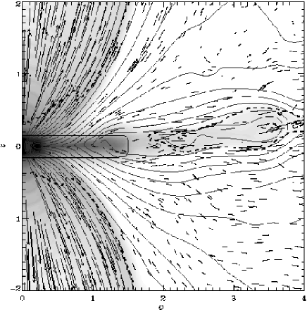
Figure 21: Poloidal velocity vectors and poloidal magnetic field lines superimposed on a grey-scale image of the logarithmic density. Dark means high density. The thick dashed line denotes the location where the poloidal flow speed equals the fast magnetosonic speed. The thin solid line gives the location of the disc surface. The slight asymmetry in the field is a relic from the mixed-parity initial condition. [Adapted from Brandenburg (2000).]

In figure 21 we present a particular model of Dobler et al. (1999) and Brandenburg (2000); see Brandenburg et al. (2000) for a full account of this work. In these models the outflow is driven by mass sources whose strength is proportional to the local density deficit relative to that in the original equilibrium solution of the disc. Such a density deficit was initially caused by slow gas motions that resulted from an instability of the initial equilibrium solution, because a cool disc embedded in a hot corona is nonrotating outside the disc, and it is the resulting vertical shear profile that causes the instability (cf. Urpin & Brandenburg 1998). At later times, of course, the outflow makes the corona corotating, but by that time the outflow is driven by a persistent density deficit in the disc relative to the initial references solution.

In this model the magnetic field was generated by an $\alpha-\Omega$ dynamo operating within the disc. However $\alpha$ is negative in the upper disc plane (see Brandenburg et al. 1995), and then the most preferred field geometry is dipolar (Campbell 1999, v. Rekowski, Rüdiger, & Elstner 2000). The field parity is sensitive to details in the disc physics assumed in the particular model (aspect ratio, disc thickness, the presence of outflows, and the conductivity in the disc and the exterior). Nevertheless, both dipolar and quadrupolar fields are equally well able to contribute to wind launching, at least in the outer parts of the disc where the angle between the field and the disc plane is less than $60^{\circ}$, the critical angle for magneto-centrifugal wind launching (Blandford & Payne 1982). We note, however, that the more detailed analysis of Campbell (1999) suggests that the critical angle can be significantly smaller.

In our models the outflow is only weakly collimated (if at all). This is probably connected with the fact that here the fast magnetosonic surface is rather close to the disc surface, making it difficult for the field to become strong enough to channel the magnetic field. Instead, the field lines themselves are still being controlled too strongly by the outflow. However, outflows with rather large opening angles are actually seen in some star-forming regions; see Greenhill et al. (1998).

While most of the disc mass is ejected in a cone of half-opening angle around $25^{\circ}$, most of the disc angular momentum is ejected at rather low latitudes, almost in the direction of the disc plane away from the central object. The timescales for these various processes are comparable. In figure 22 we show the azimuthally integrated mass flux, angular momentum flux, and magnetic (Poynting) flux as a function of polar angle, and compare with a nonmagnetic run. We find that in the magnetic run the outflow is more strongly concentrated towards the axis. Also, the amount of angular momentum loss (dash-dotted line) is larger when the disc is magnetized. We emphasize in particular that in the magnetic run significant amounts of magnetic field are eject from the system. In the following section we discuss the significance of such magnetic flux ejection for magnetizing the interstellar medium into which the outflow is streaming. This discussion is similar to a corresponding discussion for the contamination of the intergalactic medium via outflows from active galactic nuclei (Brandenburg 2000).

Figure 22: Comparison of the angular dependence of azimuthally integrated fluxes for magnetic and nonmagnetic outflows. The solid line refers to mass flux, the dashed line to angular momentum flux, and the dash-dotted line (in the second panel) corresponds to the Poynting flux. The units of all quantities are thus $1/[t]$.

6.4 Magnetic contamination from outflows

It may at first appear somewhat unrealistic to expect significant magnetization of the interstellar medium from outflows. However, the following calculation shows that the effect may be quite significant. Assume that every star did undergo a phase of strong accretion with associated outflows, so $N=10^{11}$ for the whole galaxy. The duration of intense outflow activity is $10^{5}$ years, say, but it could even be $10^{6}$ years. The magnetic luminosity is $L_{\rm mag}=0.05\dot{M}_{\rm w}c_{\rm s}^{2}$ (Brandenburg et al. 2000), where $c_{\rm s}\approx 10\,{\rm km/s}$ is the average sound speed of the interstellar medium, and $\dot{M}_{\rm w}=0.1\dot{M}_{\rm d}$ (see Pelletier & Pudritz 1992), where $\dot{M}_{\rm d}\approx 10^{-7}M_{\odot}/\,{\rm yr}$ is a conservative estimate for the disc accretion rate. Again this value may be larger. With the above numbers the magnetic luminosity from all $N=10^{11}$ sources is then $NL_{\rm mag}=7\times 10^{39}\,{\rm erg}/\,{\rm s}$ and the total energy output delivered from all stars at some early point in the life time is therefore $E_{\rm mag}=\tau NL_{\rm mag}=2\times 10^{52}\,{\rm erg}$. Diluting this over a volume of a galaxy of $300\,{\rm kpc}^{3}$ (radius 10 kpc, height 1 kpc) gives $2\times 10^{-15}\,{\rm erg}/\,{\rm cm}^{3}$. Multiplying this by $8\pi$ and taking the square root gives $0.2\mu G$. Expressed more concisely in a formula we have for the rms magnetic field strength

$$\langle\mbox{\boldmath$B$}{}^{2}\rangle^{1/2}\approx\left(8\pi\,{F_{\rm Poy}\over F_{\rm kin}}\,{N\dot{M}_{\rm w}c_{\rm s}^{2}\over V}\,\delta t\right)^{1/2},$$ (157)

where the efficiency factor $F_{\rm Poy}/F_{\rm kin}$ (=0.05 in our model) may be lower in systems where the disc dynamo is less strong.

The parameters for a corresponding estimate for outflows from young galactic discs (active galactic nuclei) are as follows. Assuming $N\sim 10^{4}$ galaxies per cluster, each with $\dot{M}_{\rm w}\approx 0.1M_{\odot}/{\rm yr}=10^{25}\,{\rm g/s}$, and $c_{\rm s}=1000\,{\rm km/s}$ for the sound speed in the intracluster gas, the rate of magnetic energy injection for all galaxies together is $L_{\rm mag}=10^{44}\,{\rm erg/s}$. Distributing this over the volume of the cluster of $V\sim 1\,{\rm Mpc}^{3}$, and integrating over a duration of $\delta t=1\,{\rm Gyr}$, this corresponds to a mean magnetic energy density of $\langle\mbox{\boldmath$B$}{}^{2}/8\pi\rangle\approx 10^{-13}\,{\rm erg}/{\rm cm}^{3}$, so $\langle\mbox{\boldmath$B$}{}^{2}\rangle^{1/2}\approx 10^{-6}\,{\rm G}$, which is indeed of the order of the field strength observed in galaxy clusters. We note that our estimate has been rather optimistic in places ($\dot{M}_{\rm w}$ could be lower, or the relevant $\delta t$ could be shorter, for example), but it does show that outflows are bound to produce significant magnetization of the intracluster gas and the interstellar medium (see also Völk & Atoyan 1999). In the latter case it will provide a good seed field for the galactic dynamo. A dynamo is still necessary to shape the magnetic field and to prevent if from decaying in the galactic turbulence. Similarly, many galaxy clusters undergo merging and this too can enhance and reorganize the magnetic field. The necessity for a recent merger event would also be consistent with the fact that not all halos are observed to have strong magnetic fields. Recent simulations by Roettiger, Stone & Burns (1999) suggest that after a merger the field strength may increase by a factor of at least 20 (and this value increases with improving observational resolution).

As an alternative consideration for causing the magnetization in clusters of galaxies, primordial magnetic fields are sometimes discussed. There are numerous mechanisms that could generate relatively strong fields at an early time, for example during inflation (age $\sim 10^{-36}\,{\rm s}$) or during the electroweak phase transition (age $\sim 10^{-10}\,{\rm s}$). Such fields would now still be at a very small scale if one considers only the cosmological expansion. However, depending on the degree of magnetic helicity in this primordial field, the magnetic energy can be transferred to larger scales that are now on the scale of galaxies. For a recent discussion of these results see Brandenburg (2001a).

7 Hydromagnetic turbulence and dynamos

As mentioned in the beginning, accurate high order schemes are essential in all applications to turbulent flows. Nevertheless, we should mention that one often attempts solutions of the inviscid and nonresistive equations using low-order finite differences combined with monotonicity schemes that result in some kind of effective diffusion. The piece-wise parabolic method (PPM) of Colella & Woodward (1984) is an example. However, unlike the Smagorinsky scheme (see Chan & Sofia 1986, 1989, Steffen, Ludwig, & Krüß 1989, Fox, Theobald, & Sofia 1991 for applications to convection simulations), PPM and similar methods cannot be proven to converge to the original Navier-Stokes equation in the limit of infinite resolution. Nevertheless, they are rather popular in astrophysical gas simulations. These schemes are rather robust and have also been applied to high resolution simulations of compressible turbulence (Porter, Pouquet, & Woodward 1992, 1994). While the results from those simulations are generally quite plausible, the power spectrum shows a $k^{-1}$ subrange at large wave numbers, which is still not fully understood. This was sometimes regarded as an artifact of PPM, and should therefore only occur at small scales. However, as the resolution was increased further (up to $1024^{3}$), the $k^{-1}$ subrange just became more extended.

A similar feature was found in cascade models of turbulence when the ordinary $\nabla^{2}$ diffusion operator was replaced by a $-\nabla^{4}$ “hyperdiffusion” operator (Lohse & Müller-Groeling 1995). Whatever the outcome of this puzzle is, it is clear that with schemes that cannot be proven to converge to the actual Navier-Stokes equations in the limit of infinite resolution, there would always remain some uncertainty and debate. On the other hand, especially in the incompressible case the use of hyperviscosity does generally allow the exploration of larger Reynolds numbers and broader inertial ranges.

MHD simulations with the highest resolution to date have been performed by Biskamp & Müller (1999), who considered decaying turbulence with and without magnetic helicity. They found that in the presence of magnetic helicity the magnetic energy decay is significantly slower. In particular, they found the magnetic energy decays like $t^{-1/2}$, as opposed to $t^{-1}$ found earlier by Mac Low, Klessen, & Burkert (1998) for compressible turbulence.

Before we start discussing dynamo action in turbulence simulations representative of more astrophysical settings, such as accretion discs and the solar convection zone, let us first illustrate the mechanism of the inverse cascade that is believed to be an important ingredient of large scale magnetic field generation.

7.1 Isotropic MHD turbulence

Most developments in the theory of turbulence have been carried out under the assumptions of homogeneity and isotropy. This is certainly true of the work on the inverse cascade (or turbulent cascades in general), but it is also true of much of the work on the $\alpha$-effect which – like the inverse cascade – describes the generation of large scale fields. However, unlike the inverse cascade process, the energy comes here directly from the velocity field at the scales of the energy-carrying eddies and not from the velocity and magnetic field at successively smaller scales, which are usually larger than the scale of the energy-carrying eddies.

It is not easy to see whether any of these effects is actually responsible for the large scale field generation in astrophysical bodies or even the simulations. In simulations of accretion disc turbulence there is certainly some evidence for the presence of an $\alpha$-effect, but it is extremely noisy (Brandenburg et al. 1995, Brandenburg & Donner 1997, Ziegler & Rüdiger 2000). Evidence for the inverse magnetic cascade comes mostly from the magnetic energy spectra (Balsara & Pouquet 1999, Brandenburg 2001b), which show a marked peak at large scales, but this is convincing only in cases where the flow is driven at a wavenumber that is clearly larger than the smallest wavenumber in the box. In practice, e.g. in convectively driven turbulence, the flow is driven at all scales including the large scale making it difficult to see a marked peak at the smallest wavenumber (see a corresponding discussion in Meneguzzi & Pouquet 1989).

From the seminal papers of Frisch et al. (1975) and Pouquet, Frisch, Léorat (1976) it is clear that amplification of large scale fields can also be explained by an inverse cascade of magnetic helicity. In those papers the authors also showed that the inverse cascade is a consequence of the fact that the magnetic helicity, $\langle\mbox{\boldmath$A$}{}\cdot\mbox{\boldmath$B$}{}\rangle$, is conserved by the nonresistive equations. ($A$ is the magnetic vector potential giving the magnetic field as $\mbox{\boldmath$B$}{}=\mbox{\boldmath$\nabla$}{}\times\mbox{\boldmath$A$}{}$.) The inverse magnetic cascade effect too is rather difficult to isolate in simulations of astrophysical turbulence. However, under somewhat more idealized conditions, for example when magnetic energy is injected at high wave numbers, one clearly sees how the magnetic energy increases at large scales; see figure 23. Further details of this model have been published in the proceedings of the helicity meeting in Boulder (Brandenburg 1999).

Figure 23: Spectral magnetic energy, $E_{\rm M}(k,t)$, as a function of wavenumber $k$ for different times: dotted lines are for early times ($t=2,4,10,20$), the solid and dashed lines are for $t=40$ and 60, respectively, and the dotted-dashed lines are for later times ($t=80,100,200,400$). Here magnetic energy is injected at wavenumber 10. Note the occurrence of a sharp secondary peak of spectral magnetic energy at $k=10$. By the time the energy at $k=1$ has reached equipartition the energies in $k=2$ and $k=4$ become suppressed.

In the model considered above the flow was forced magnetically. This may be motivated by the recent realization that strong magnetic field generation in accretion discs can be facilitated by magnetic instabilities, such as the Balbus-Hawley instability. Other examples of magnetic instabilities include the magnetic buoyancy instability, which can lead to an $\alpha$-effect (e.g. Brandenburg & Schmitt 1998, Thelen 2000), and the reversed field pinch which also leads to a dynamo effect (e.g. Ji et al. 1996). Before returning to the accretion disc dynamo in § 7.9 we should emphasize that strong large scale field generation is also possible with purely hydrodynamic forcing. Simulations in this type were considered recently by Brandenburg (2001b). There are many similarities compared with the case of magnetic forcing. The evolution of magnetic energy spectra in the presence of hydrodynamic forcing is shown in figure 24. Like in the case of magnetic forcing (figure 23) there are marked peaks both at the forcing scale and at the largest scale of the box. Furthermore, the evolution of spectral energy at the largest scales shows similar behavior: the magnetic energy with wavenumber $k=8$ increases, reaches a maximum, and begins to decrease when the magnetic energy at $k=4$ reaches a maximum. The same happens for the next larger scales (wavenumbers $k=4$ and 2, until the scale of the box (with $k=1$) is reached.

Figure 24: Left: magnetic energy spectra for a run with forcing at $k=30$. The times range from 0 (dotted line) to 10, 30, …, 290 (solid lines). The thick solid line gives the final state at $t=1000$. Note that at early times the spectra peaks at $k_{\max}\approx 7$. The $k^{-1}$ and $k^{+3/2}$ slopes are given for orientation as dash-dotted lines. Right: evolution of spectral magnetic energy for selected wavenumbers in a simulation with hydrodynamical forcing at $k=30$.

The suppression of magnetic energy at intermediate scales, $2\leq k\leq 8$, is quite essential for the development of a well-defined large scale field. In a recent letter Brandenburg & Subramanian (2000) showed that this type of self-cleaning effect can also be simulated by using ambipolar diffusion as nonlinearity and ignoring the Lorentz force altogether. Without any nonlinearity, however, there would be no interaction between different scales and the magnetic energy would increase at all scales, especially at small scales, which would soon swamp the large scale field structure with small scale fields.

The model presented in figure 24 has large scale separation in the sense that there is a large gap between the forcing wavenumber ($k=k_{\rm f}=30$) and the wavenumber of the box ($k=k_{1}=1$). One sees that during the growth phase there is a clear secondary maximum at $k=7$. This is indeed expected for an $\alpha^{2}$ dynamo, whose maximum growth rate is at $k_{\max}={\textstyle{1\over 2}}\alpha/\eta_{\rm T}$, where $\eta_{\rm T}$ is the total (turbulent plus microscopic) magnetic diffusion coefficient.

The disadvantage of a high forcing wavenumber is that for modest resolution (here we used $120^{3}$ meshpoints) no inertial range can develop. This is different if once forces at $k_{\rm f}=5$, keeping otherwise the same resolution. In figure 25 we show spectra for different cases with $k_{\rm f}=5$ where we compare the results for different values of the magnetic Reynolds and magnetic Prandtl number. In figure 26 we show cross-sections of one field component at different times. In this model (Run 3 of Brandenburg 2001b) the forcing is at $k_{\rm f}=5$, so there is now a clear tendency for the build-up of an inertial range in $8\leq k\leq 25$.

Figure 25: Comparison of time averaged magnetic energy spectra for Runs 1–3 ($t=600-1000$) with a non-averaged spectrum for Run 5 (large magnetic Prandtl number) taken at $t=1600$. To compensate for different field strengths and to make the spectra overlap at large scales, two of the three spectra have been multiplied by a scaling factor. There are clear signs of the gradual development of an inertial subrange for wavenumbers larger than the forcing scale. The $k^{-5/3}$ slope is shown for orientation. The dissipative magnetic cutoff wavenumbers, $\langle\mbox{\boldmath$J$}{}^{2}/\eta^{2}\rangle^{1/4}$, are indicated by arrows at the top.

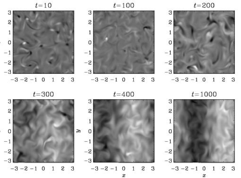
Figure 26: Gray-scale images of cross-sections of $B_{x}(x,y,0)$ for Run 3 of Brandenburg 2001b at different times showing the gradual build-up of the large scale magnetic field after $t=300$. Dark (light) corresponds to negative (positive) values. Each image is scaled with respect to its min and max values.

7.2 The inverse cascade in decaying turbulence

We now turn to the case of decaying turbulence, which is driven only by an initial kick to the system. There are several circumstances in astrophysics where this could be relevant: early universe, neutron stars, and mergers of galaxy clusters. In all those cases one is interested in the development of large scale fields. In the context of the early universe the possibility of energy conversion from small to large scale fields was pointed out by Brandenburg, Enqvist, & Olesen (1996) who found that fields generated at the horizon scale of $3\,{\rm cm}$ after the electroweak phase transition would now have a scale on the order of kiloparsecs, even though the cosmological expansion alone would only lead to scales on the order of $1\,{\rm AU}$. These results were only based on either two-dimensional simulations or three-dimensional cascade model calculation (e.g. Biskamp 1994). Therefore we now turn to fully three-dimensional simulations.

In the absence of any forcing and with no kinetic energy initially an initial magnetic field can only decay. However, if initially most of the magnetic energy is in the small scales, there is the possibility that magnetic helicity and thereby also magnetic energy is transferred to large scales. This is exactly what happens (figure 27), provided there is initially some net helicity. The inset of figure 27 shows that in the absence of initial net helicity the field at large scales remains unchanged, until diffusion kicks in and destroys the remaining field at very late times.

Figure 27: Power spectra of magnetic energy (solid lines) and kinetic energy (dotted lines) in a decay run with helicity. The left hand panel is for a case where the flow is only driven by an initial helical magnetic field. In the right hand panel the field is weak and governed by strong decaying fluid turbulence. The inset shows both velocity and magnetic spectra in the same plot. The Prandtl number $\nu/\eta$ is equal to one in both cases, but the mesh Reynolds number, which is kept constant at all times, is different in the two cases: 20 in the left hand panel and 50 in the right hand panel. The times are 0, 0.01, 0.1, etc, till $t=10^{2}$ in the left hand panel and $t=10^{3}$ in the right hand panel.

If the magnetic field has the possibility to tap energy also from the large scale velocity the situation is somewhat different again and there is the possibility that a large scale magnetic field can also be driven without net helicity. In that case the large scale field can increase due to dynamo action from the incoherent $\alpha-\Omega$-effect (Vishniac & Brandenburg 1997). In astrophysical settings there is usually large scale shear from which energy can be tapped. Before we discuss simulations with imposed shear in more detail we first present a simple argument that makes the link between the inverse cascade and helicity conservation.

7.3 The connection with magnetic helicity conservation

In the following we give a simple argument due to Frisch et al. (1975) that helps to understand why the magnetic helicity conservation property leads to the occurrence of an inverse cascade. We define in the following magnetic energy and helicity spectra, $M(k)$ and $H(k)$, respectively. Now, because of Schwartz inequality, we have

$$|\hat{\mbox{\boldmath$B$}}{}(k)|^{2}=|(i\mbox{\boldmath$k$}{}\times\hat{\mbox{\boldmath$A$}}{})\cdot\hat{\mbox{\boldmath$B$}}{}|\geq|\mbox{\boldmath$k$}{}||\hat{\mbox{\boldmath$A$}}{}\cdot\hat{\mbox{\boldmath$B$}}{}|$$ (158)

we have a lower bound on the spectral magnetic energy at each wavenumber $k=\mbox{\boldmath$k$}{}$. In terms of shell integrated magnetic energy and helicity spectra this corresponds to

$$M(k)\geq{\textstyle{1\over 2}}k|H(k)|,$$ (159)

where the 1/2-factor comes simply from the 1/2-factor in the definition of the magnetic energy. Assuming that two wave numbers $q$ and $p$ interact such that they produce power at a new wave number $k$, then

$$M(p)+M(q)=M(k),\quad H(p)+H(q)=H(k).$$ (160)

For simplicity we consider the case $p=q$, so

$$2M(p)=M(k),\quad 2H(p)=H(k).$$ (161)

Assume also that initially the constraint was sharp (maximum helicity), then

$$M(p)={\textstyle{1\over 2}}pH(p).$$ (162)

Now, from the constrain again we have

$${\textstyle{1\over 2}}kH(k)\leq M(k)=2M(p)=pH(p)={\textstyle{1\over 2}}pH(k),$$ (163)

so

$$k\leq p,$$ (164)

that is the wave number of the target result must be larger or equal to the wave numbers of the initial field.

The argument given above is of course quite rough, because it ignores for example the detailed angular dependence of the wave vectors. This was taken into account properly already in the early paper by Pouquet, Frisch, & Léorat (1976), but this approach was based on closure assumptions for the higher moments, which is in principle open to criticism. Thus, numerical simulations, like those presented above, are necessary for an independent confirmation that the inverse cascade really works. In this connection one should mention that there are some parallels with the inverse cascade of enstrophy in two-dimensional hydrodynamic (nonmagnetic) turbulence. In that case the enstrophy (i.e. the mean squared vorticity) is conserved because of the absence of vortex stretching in two dimensions. The inverse hydrodynamic cascade has some significance in meteorology and perhaps in low aspect ratio convection experiments, where one finds a peculiar energy and entropy spectrum that is referred to as Bolgiano scaling; see Brandenburg (1992) and Suzuki & Toh (1995) for corresponding shell model calculations and Toh & Iima (2000) for direct simulations.

7.4 Inverse cascade or $\alpha$-effect?

In § 7.1 we made a distinction between inverse cascade and $\alpha$-effect in the sense that, although both lead to large scale field generation, in the inverse cascade there is a gradual transfer of magnetic helicity and energy to ever larger scales, whereas the $\alpha$-effect produces large scale magnetic fields directly from small scale fields. Thus, the distinction is really one between local and nonlocal inverse cascades.

In figure 28 we show the normalized spectral energy transfer function $T(k,p,t)$ for $k=1$ and 2 as a function of $p$, and at different times $t$. The index $k$ signifies the gain or losses of the field at wavenumber $k$, and the index $p$ indicates the wavenumber of the velocity from which the energy comes from. This function shows that most of the energy of the large scale field at $k=1$ comes from velocity and magnetic field fluctuations at the forcing scale, which is here $k=k_{\rm f}=5$. At early times this is also true of the energy of the magnetic field at $k=2$, but at late times, $t=1000$, the gain from the forcing scale, $k=5$, has diminished, and instead there is now a net loss of energy into the next larger scale, $k=3$, suggestive of a direct cascade operating at $k=2$, and similarly at $k=3$.

Figure 28: Spectral energy transfer function $T(k,p,t)$, normalized by $\langle\mbox{\boldmath$B$}{}^{2}\rangle$ for three different times, for $k=1$ and 2. Run 3 of Brandenburg (2001b).

Based on these results we may conclude that in the saturated state the magnetic energy at $k=1$ is sustained by a nonlocal inverse cascade from the forcing scale directly to the largest scale of the box. This is characteristic of the $\alpha$-effect of mean-field electrodynamics, except that here nonlinearity plays an essential role in isolating the large scale from the small scale ‘magnetic trash’, as Parker used to say.

A closer look at figure 24, where $k=k_{\rm f}=30$, suggests that once the scale separation is large enough the energy is at first transferred not to the scale of the box, but instead to a somewhat smaller scale (here at wavenumber $k=7$). Following the corresponding discussion in Brandenburg (2001b), this wavenumber is close to the wavenumber, $k_{\max}={\textstyle{1\over 2}}|\alpha|/\eta_{\rm T}$, where the $\alpha^{2}$ dynamo grows fastest.

In the following section we address the issue of magnetic helicity conservation which has important consequences for the timescale after which the large scale field begins to develop. This has also a bearing on the widely discussed controversy of the so-called ‘catastrophic $\alpha$-quenching’ of Vainshtein & Cattaneo (1992).

7.5 Approximate helicity conservation

The magnetic helicity, $H=\langle\mbox{\boldmath$A$}{}\cdot\mbox{\boldmath$B$}{}\rangle$, is conserved by the nonresistive MHD equations. For a closed or periodic box $\langle\mbox{\boldmath$A$}{}\cdot\mbox{\boldmath$B$}{}\rangle$ satisfies the equation

$${{\rm d}{}\over{\rm d}{}t}\langle\mbox{\boldmath$A$}{}\cdot\mbox{\boldmath$B$}{}\rangle=-2\eta\mu_{0}\langle\mbox{\boldmath$J$}{}\cdot\mbox{\boldmath$B$}{}\rangle,$$ (165)

where $\langle\mbox{\boldmath$J$}{}\cdot\mbox{\boldmath$B$}{}\rangle$ is the current helicity, and angular brackets denote volume averages. Note that for a periodic box $\langle\mbox{\boldmath$A$}{}\cdot\mbox{\boldmath$B$}{}\rangle$ is gauge invariant, i.e. $\langle\mbox{\boldmath$A$}{}\cdot\mbox{\boldmath$B$}{}\rangle$ does not change after a gauge transformation, $\mbox{\boldmath$A$}{}\rightarrow\mbox{\boldmath$A$}{}+\mbox{\boldmath$\nabla$}{}\varphi$. This is a direct consequence of the solenoidality of the magnetic field, because $\langle\mbox{\boldmath$\nabla$}{}\varphi\cdot\mbox{\boldmath$B$}{}\rangle=-\langle\varphi\mbox{\boldmath$\nabla$}{}\cdot\mbox{\boldmath$B$}{}\rangle=0$ owing to $\mbox{\boldmath$\nabla$}{}\cdot\mbox{\boldmath$B$}{}=0$.

In order to judge whether $\langle\mbox{\boldmath$A$}{}\cdot\mbox{\boldmath$B$}{}\rangle$ is small or large we calculate the length scale

$$\ell_{\rm H}=|\langle\mbox{\boldmath$A$}{}\cdot\mbox{\boldmath$B$}{}\rangle|/\langle\mbox{\boldmath$B$}{}^{2}\rangle.$$ (166)

In figure 29 we see that the evolution of $\ell_{\rm H}$ proceeds in three distinct phases: (i) a very short period ($t<1$) where $\ell_{\rm H}$ is very small and comparable to the numerical noise level, so magnetic helicity almost perfectly conserved, (ii) an intermediate interval ($2<t<200$) where $\ell_{\rm H}$ is much larger, but still only roughly equal to the mesh size of the calculation, and then (iii) a regime where $\ell_{\rm H}$ is of order unity. The latter is only possible because of the presence of helicity in the system, which leads to a large scale magnetic field configuration that is nearly force-free.

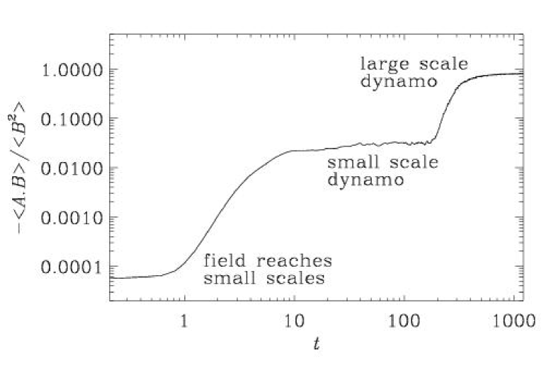
Figure 29: Evolution of the (negative) magnetic helicity length scale in a double-logarithmic plot. Note the presence of three distinct phases: very approximate helicity conservation near zero, followed by a phase of larger magnetic helicity scale (three orders of magnitude), and finally a phase where the magnetic helicity scale has reached the scale of the box.

7.6 Resistively limited growth of the large scale field

The approximate conservation of magnetic helicity has an important consequence for the generation of large scale fields: in order to build up a large scale field with magnetic helicity one has to change the value of $\langle\mbox{\boldmath$A$}{}\cdot\mbox{\boldmath$B$}{}\rangle$ from its initial value of zero to its certain final value. This final value of $\langle\mbox{\boldmath$A$}{}\cdot\mbox{\boldmath$B$}{}\rangle$ is such that the length scale $\ell_{\rm H}$ is close to the maximum value possible for a certain geometry. It also implies that when interpreting the results in terms of mean-field electrodynamics ($\alpha$-effect and turbulent diffusion), the $\alpha$-effect must be quenched early on, well before the field has reached its final value. Nevertheless, this strong quenching, which was first anticipated by Vainshtein & Cattaneo (1992) and later confirmed numerically by Cattaneo & Hughes (1996), does not prevent the field from reaching its final super-equipartition field strength.

Before we come to the details we mention already now that the helicity constraint is probably too severe to be acceptable for astrophysical conditions, so one must look for possible escape routes. The most plausible way of relaxing the helicity constraint is in allowing for open boundary conditions (Blackman & Field 2000, Kleeorin et al. 2000), but the situation can still be regarded as inconclusive. Given that much of the work on large scale dynamos so far assumes periodic boundaries, we shall now consider this particular case in more detail. In the periodic case the final field geometry can be, for example, of the form $\overline{\mbox{\boldmath$B$}}=B_{0}(\cos k_{1}z,\sin k_{1}z,0)$, where $k_{1}=1$ is the smallest possible wavenumber in the box, $B_{0}$ is the field amplitude, and $\langle\overline{\mbox{\boldmath$B$}}^{2}\rangle=B_{0}^{2}$. Alternatively, the field may vary in the $x$ or $y$ direction, and there may be an arbitrary phase shift; examples of these possibilities have been reported in Brandenburg (2001b). Anyway, for $\overline{\mbox{\boldmath$B$}}=B_{0}(\cos k_{1}z,\sin k_{1}z,0)$ the corresponding vector potential is $\overline{\mbox{\boldmath$A$}}=-(B_{0}/k_{1})(\cos k_{1}z,\sin k_{1}z,0)+\mbox{\boldmath$\nabla$}{}\phi$, where $\phi$ is an arbitrary gauge which does not affect the value of $\langle\overline{\mbox{\boldmath$A$}}\cdot\overline{\mbox{\boldmath$B$}}\rangle$. In this example we have

$$\langle\overline{\mbox{\boldmath$A$}}\cdot\overline{\mbox{\boldmath$B$}}\rangle=-\langle\overline{\mbox{\boldmath$B$}}^{2}\rangle/k_{1},$$ (167)

where we have included the $k_{1}$ factor, even though in the present case $k_{1}$=1. (The minus sign in eq. (167) would turn into a plus if the forcing had negative helicity.) The mean current density is given by $\overline{\mbox{\boldmath$J$}}=-B_{0}k_{1}(\cos k_{1}z,\sin k_{1}z,0)$, so the current helicity of the mean field is given by

$$\mu_{0}\langle\overline{\mbox{\boldmath$J$}}\cdot\overline{\mbox{\boldmath$B$}}\rangle=-k_{1}\langle\overline{\mbox{\boldmath$B$}}^{2}\rangle.$$ (168)

Before we can use eqs. (167) and (168) in eq. (165) we need to relate the magnetic and current helicities of the mean field to those of the actual field. We can generally split up the two helicities into contributions from large and small scales, i.e.

$$\langle\mbox{\boldmath$A$}{}\cdot\mbox{\boldmath$B$}{}\rangle=\langle\overline{\mbox{\boldmath$A$}}\cdot\overline{\mbox{\boldmath$B$}}\rangle+\langle\mbox{\boldmath$a$}{}\cdot\mbox{\boldmath$b$}{}\rangle,$$ (169)

$$\langle\mbox{\boldmath$J$}{}\cdot\mbox{\boldmath$B$}{}\rangle=\langle\overline{\mbox{\boldmath$J$}}\cdot\overline{\mbox{\boldmath$B$}}\rangle+\langle\mbox{\boldmath$j$}{}\cdot\mbox{\boldmath$b$}{}\rangle.$$ (170)

As the large scale magnetic field begins to saturate, the magnetic helicity has to become constant and so eq. (165) dictates that $\langle\mbox{\boldmath$J$}{}\cdot\mbox{\boldmath$B$}{}\rangle$ must go to zero in the steady state. Consequently, the contribution from $\langle\mbox{\boldmath$j$}{}\cdot\mbox{\boldmath$b$}{}\rangle$ must be as large as that of $\langle\overline{\mbox{\boldmath$J$}}\cdot\overline{\mbox{\boldmath$B$}}\rangle$, and of opposite sign, so that the two cancel. This, together with eq. (168), allows us immediately to write down an expression for the equilibrium strength of the mean field;

$$\langle\overline{\mbox{\boldmath$B$}}^{2}\rangle=\mu_{0}|\langle\mbox{\boldmath$j$}{}\cdot\mbox{\boldmath$b$}{}\rangle|/k_{1},$$ (171)

which is now valid for both signs of the helicity of the forcing. The residual helicity (Pouquet, Frisch, Léorat 1976),

$$H_{\rm res}=\langle\mbox{\boldmath$\omega$}{}\cdot\mbox{\boldmath$u$}{}\rangle-\langle\mbox{\boldmath$j$}{}\cdot\mbox{\boldmath$b$}{}\rangle/\rho_{0},$$ (172)

is small in the nonlinear saturated state and nearly vanishing. [We mention that this is also the case in the models of Brandenburg & Subramanian (2000).] Furthermore, for forced turbulence with a well defined forcing wavenumber the kinetic helicity may be estimated as $\langle\mbox{\boldmath$\omega$}{}\cdot\mbox{\boldmath$u$}{}\rangle\approx k_{\rm f}\langle\mbox{\boldmath$u$}{}^{2}\rangle$. Together with eq. (171) we have

$$\langle\overline{\mbox{\boldmath$B$}}^{2}\rangle={k_{f}\over k_{\rm 1}}\,B_{\rm eq}^{2},$$ (173)

where $B_{\rm eq}^{2}=\mu_{0}\langle\rho\mbox{\boldmath$u$}{}^{2}\rangle$ and $B_{\rm eq}$ is the equipartition field strength. Thus, the mean field can exceed (!) the equipartition field by the factor $(k_{f}/k_{\rm 1})^{1/2}$. This estimate agrees well with the results of the simulations; see Brandenburg (2001b).

Using eqs. (169) and (170) together with eqs. (167) and (168) we can rewrite eq. (165) in the form

$${{\rm d}{}\over{\rm d}{}t}\langle\overline{\mbox{\boldmath$B$}}^{2}\rangle=-2\eta k_{1}^{2}\langle\overline{\mbox{\boldmath$B$}}^{2}\rangle+2\eta k_{1}\mu_{0}|\langle\mbox{\boldmath$j$}{}\cdot\mbox{\boldmath$b$}{}\rangle|,$$ (174)

where we have taken into account the contribution of the small scale current helicity which is of similar magnitude as the large scale current helicity. For the magnetic helicity, on the other hand, the small scale contribution is negligible, because

$$|\langle\mbox{\boldmath$a$}{}\cdot\mbox{\boldmath$b$}{}\rangle|\approx\mu_{0}|\langle\mbox{\boldmath$j$}{}\cdot\mbox{\boldmath$b$}{}\rangle|/k_{\rm f}^{2}\approx\mu_{0}|\langle\overline{\mbox{\boldmath$J$}}\cdot\overline{\mbox{\boldmath$B$}}\rangle|/k_{\rm f}^{2}\approx|\langle\overline{\mbox{\boldmath$A$}}\cdot\overline{\mbox{\boldmath$B$}}\rangle|\left({k_{1}\over k_{\rm f}}\right)^{2}\ll|\langle\overline{\mbox{\boldmath$A$}}\cdot\overline{\mbox{\boldmath$B$}}\rangle|.$$ (175)

After the saturation at small and intermediate scales the small scale current helicity is approximately constant and can be estimated as

$$|\langle\mbox{\boldmath$j$}{}\cdot\mbox{\boldmath$b$}{}\rangle|\approx\rho_{0}|\langle\mbox{\boldmath$\omega$}{}\cdot\mbox{\boldmath$u$}{}\rangle|\approx k_{\rm f}\langle\rho\mbox{\boldmath$u$}{}^{2}\rangle=k_{\rm f}B_{\rm eq}^{2}/\mu_{0}.$$ (176)

The solution of (174) is given by

$$\langle\overline{\mbox{\boldmath$B$}}^{2}\rangle=\epsilon_{0}B_{\rm eq}^{2}\left[1-e^{-2\eta k_{1}^{2}(t-t_{\rm sat})}\right],$$ (177)

where $\epsilon_{0}$ is a coefficient which, in the present model with a well-defined forcing wavenumber, can be approximated by $\epsilon_{0}\approx k_{\rm f}/k_{1}$.

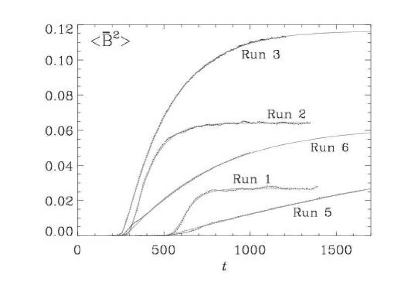
Figure 30: Evolution of $\langle\overline{\mbox{\boldmath$B$}}^{2}\rangle$ for Runs 1–3, 5, and 6, compared with the solution (179) of the dynamo equations using eq. (179).

This is indeed also the limiting behavior found for $\alpha^{2}$-dynamos with simultaneous $\alpha$ and $\eta$ quenching of the form

$$\alpha={\alpha_{0}\over 1+\alpha_{B}\overline{\mbox{\boldmath$B$}}^{2}\!/B_{\rm eq}^{2}},\quad\eta_{\rm t}={\eta_{\rm t0}\over 1+\eta_{B}\overline{\mbox{\boldmath$B$}}^{2}\!/B_{\rm eq}^{2}},$$ (178)

where $\alpha_{B}=\eta_{B}$ is assumed. Assuming that the magnetic energy density of the mean field, $\overline{\mbox{\boldmath$B$}}^{2}$, is approximately uniform (which is well satisfied in the simulations) we can obtain the solution $\overline{\mbox{\boldmath$B$}}=\overline{\mbox{\boldmath$B$}}(t)$ of eq. (303) in the form

$$\overline{\mbox{\boldmath$B$}}^{2}/(1-\overline{\mbox{\boldmath$B$}}^{2}\!/B_{\rm fin}^{2})^{1+\lambda/\eta k_{1}^{2}}=B_{\rm ini}^{2}\,e^{2\lambda t},$$ (179)

where

$$\lambda=|\alpha_{0}|k_{1}-\eta_{\rm T0}k_{1}^{2}$$ (180)

is the kinematic growth rate of the dynamo, $B_{\rm ini}$ is the initial field strength, and $B_{\rm fin}$ is the final field strength of the large scale field, which is related to $\alpha_{B}$ and $\eta_{B}$ via

$$\alpha_{B}=\eta_{B}={\lambda\over\eta k_{1}^{2}}\left({B_{\rm eq}\over B_{\rm fin}}\right)^{2}.$$ (181)

The full derivation is given in Appendix E. The significance of this result is that it provides an excellent fit to the numerical simulations; see figure 30 where we present the evolution of $\langle\overline{\mbox{\boldmath$B$}}^{2}\rangle$ for the different runs of Brandenburg (2001b). Equation (179) can therefore be used to extrapolate to astrophysical conditions. The time it takes to convert the small scale field generated by the small scale dynamo to a large scale field, $\tau_{\rm eq}$, increases linear with the magnetic Reynolds number, $R_{\rm m}$. Apart from some coefficients of order unity the ratio of $\tau_{\rm eq}$ to the turnover time is therefore just $R_{\rm m}$. For the sun this ratio would be $10^{8}-10^{10}$. However, before interpreting this result further one really has to know whether or not the presence of open boundary conditions could alleviate the issue of very long timescales for the mean magnetic field. Furthermore, it is not clear whether the long timescales discussed above have any bearing on the cycle period in the case of oscillatory solutions. The reason this is not so clear is because for a cyclic dynamo the magnetic helicity in each hemisphere stays always of the same sign and is only slightly modulated. It is likely that this modulation pattern is advected precisely with the meridional circulation, in which case the helicity could be nearly perfectly conserved in a lagrangian frame. This could provide an interesting clue for why the solar dynamo is migrating. The relation between meridional circulation and dynamo wave propagation has been advocated by Durney (1995) and Choudhuri, Schüssler, & Dikpati (1995), but helicity conservation would strongly lock the two aspects.

It is clear that virtually all astrophysical bodies are open, allowing for constant loss of magnetic helicity. In the case of the sun significant amounts of magnetic helicity are indeed observed at the solar surface (Berger & Ruzmaikin 2000). Significant losses of magnetic helicity are particularly obvious in the case of accretion discs which are almost always accompanied by strong outflows that can sometimes be collimated into jets. Thus, dynamo action from accretion disc turbulence would be a good candidate for clarifying the significance of open boundaries on the nature of the dynamo. Another reason why accretion disc turbulence is a fruitful topic for understanding dynamo action is because the shear is extremely strong. In the following we discuss some recent progress that has been made in this field.

7.7 Joule dissipation from mean and fluctuating fields

In an MHD flow the mean magnetic Joule dissipation per unit volume is given by

$$Q_{\rm Joule}=\eta\mu_{0}\langle\mbox{\boldmath$J$}{}^{2}\rangle.$$ (182)

Whilst in may astrophysical flows $\eta$ may be very small, $|\mbox{\boldmath$J$}{}|$ can be large so that $Q_{\rm Joule}$ remains finite even in the limit $\eta\rightarrow 0$. One example where this is very important is accretion discs, where Joule dissipation (together with viscous dissipation) are important in heating the disc. These viscous and resistive processes are indeed the only significant sources of energy supply in discs, and yet the luminosities of discs that result from the conversion of magnetic and kinetic energies into heat and radiation can be enormous. Much of the work on discs involves mean-field modelling, so it would be interesting to see how the Joule dissipation, $Q_{\rm Joule}^{\rm(mf)}$, predicted from a mean-field model,

$$Q_{\rm Joule}^{\rm(mf)}=\eta_{\rm t}\mu_{0}\langle\overline{\mbox{\boldmath$J$}}^{2}\rangle,$$ (183)

relates to the actual Joule dissipation. In figure 31 we show the evolution of actual and mean-field Joule dissipation and compare with an estimate for the rate of total energy dissipation, $B_{\rm eq}^{2}/\tau$, where $\tau$ is the turnover time. Here we have taken into account that $\eta_{\rm t}$ is ‘catastrophically’ quenched using the formulae of Brandenburg (2001) with the parameters for Run 3.

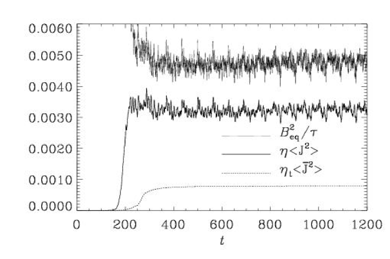
Figure 31: Joule dissipation for Run 3 (solid line), compared with the Joule dissipation estimated for a corresponding mean-field model (dashed line). An estimate for the rate of total energy dissipation, $B_{\rm eq}^{2}/\tau$, is also given.

There is no reason a priori that the magnetic energy dissipations from the mean-field model should agree with the actual one. It turns out that the mean-field dissipation is a fourth of the actual one, so it is definitely significant. It would therefore be interesting so see how those two dissipations compare with each other in other models.

7.8 Possible pitfalls in connection with hyperresistivity

In many astrophysical applications hyperresistivity and hyperviscosity are sometimes used in order to concentrate the effects of magnetic diffusion and viscosity to the smallest possible scale. The purpose of this section is to highlight possible spurious artifacts associated with this procedure. As we have seen above, large scale dynamos can depend on the microscopic magnetic diffusivity and must therefore be affected when it is replaced by hyperresistivity. The resulting modifications that are to be expected are easily understood: on the right hand side of eq. (165) the term $\langle\mbox{\boldmath$J$}{}\cdot\mbox{\boldmath$B$}{}\rangle$ needs to be replaced by $\langle(\nabla^{4}\mbox{\boldmath$A$}{})\cdot\mbox{\boldmath$B$}{}\rangle$. This leads to a change of the relative importance of small and large scale contributions, which therefore changes eq. (173) to

$$\langle\overline{\mbox{\boldmath$B$}}^{2}\rangle=\left({k_{f}\over k_{\rm 1}}\right)^{3}\,B_{\rm eq}^{2}.$$ (184)

Thus, the final field strength will be even larger than before: instead of a factor of 5 superequipartition (for $k_{\rm f}=5$) one now expects a factor of 125. Recent simulations by Brandenburg & Sarson (2001) have indeed confirmed this tendency. The main conclusion is that hyperresistivity can therefore be used to address certain issues regarding large magnetic Reynolds numbers that are otherwise still inaccessible. On the other hand, the results are in some ways distorted and need therefore be interpreted carefully.

7.9 Remarks on accretion disc turbulence

We have already mentioned the possibility of dynamo action in accretion discs. Accretion discs have been postulated some 30 years ago in order to explain the incredibly high luminosities of quasars. Only in the past few years has direct imaging of accretion discs become possible, mostly due to the Hubble Space Telescope. Accretion discs form in virtually all collapse processes, such as galaxy and star formation. In the latter case the central mass is of the order of one solar mass, while in the former it is around $10^{8}$ solar masses and is concentrated in such a small volume that that it must be a black hole. If the surrounding matter was nonrotating, it would fall radially towards the center. But this is unrealistic and even the slightest rotation relative to the central object would become important eventually as matter falls closer to the center.

Figure 32: Dependence of $\alpha_{\rm SS}$ on time and the mean magnetic field strength for a local accretion disc model (Run B of Brandenburg et al. 1996a). Here $B_{0}=\langle\mu_{0}\rho c_{\rm s}^{2}\rangle^{1/2}$ is the thermal equipartition field strength and $T_{\rm rot}=2\pi/\Omega$ the local rotation period. In the left hand panel the dotted line represents the actual data and the solid line gives the fit obtained by correlating $\alpha_{\rm SS}$ with the mean magnetic field (right hand panel).

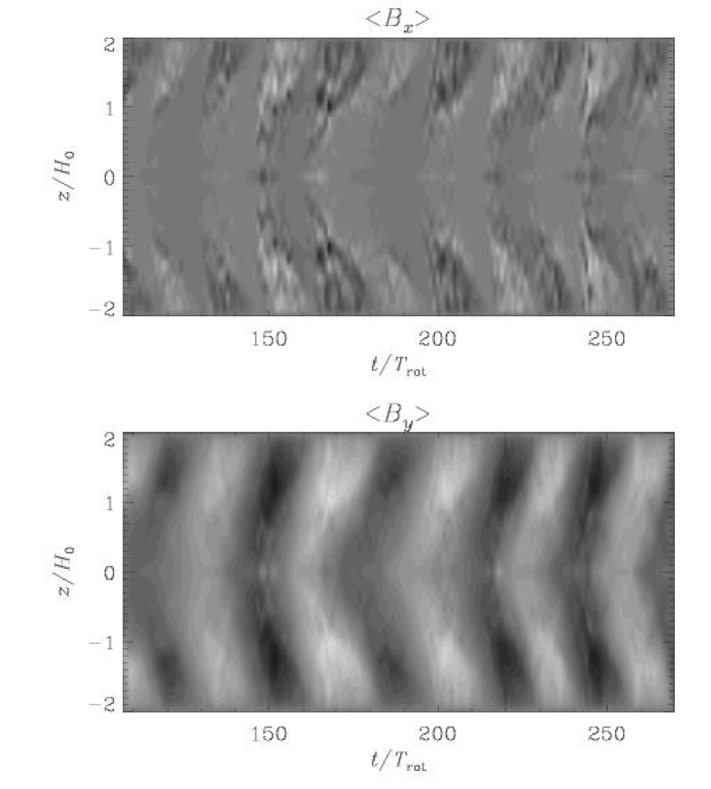
Figure 33: Butterfly (space-time) diagram of the poloidal and toroidal magnetic field components averaged over the two horizontal ($x$ and $y$) directions for the local accretion disc model of (Brandenburg et al. 1996a, Run B). Note that the poloidal field is much more noisy than the toroidal field, and that there is a clear outward migration of magnetic field.

If there was no effective diffusive process in discs, the angular momentum of the matter would stay with the gas parcels, and since the gravity force is balanced by the corresponding centrifugal force, the gas would never accrete. However, the angular velocity of the gas follows a $r^{-3/2}$ Kepler law, so the gas is differentially rotating and one may expect shear instabilities to occur that would drive turbulence and hence turbulent dissipation. Unfortunately, however, the story is not so simple. Discs are both linearly stable (Stewart 1975) and probably also nonlinearly stable (Hawley, Gammie, & Balbus 1996). Nevertheless, in the presence of a magnetic field there is a powerful linear instability (Balbus & Hawley 1991), and subsequent work has shown that this instability is indeed capable of driving the instability and hence turbulence.

One of the key outcomes of such simulations is the rate of turbulent dissipation, which determines the rate of angular momentum transport and correspondingly the rate at which orbital kinetic and potential energy is liberated in the form of heat. This is normally expressed in terms of a turbulent viscosity (e.g. Frank, King, & Raine 1992), but it may equally well be expressed in terms of the horizontal components of the Reynolds and Maxwell stress tensors. The stress may then be normalized by $\langle\rho c_{\rm s}^{2}\rangle$ to give a nondimensional measure (called $\alpha_{\rm SS}$) of the ability of the turbulence to transport angular momentum outward (if $\alpha_{\rm SS}>0$). This $\alpha_{\rm SS}$ is indeed always positive, see figure 32, but it fluctuates significantly about a certain mean value. These fluctuations are in fact correlated with the energy in the mean magnetic field, $\langle\mbox{\boldmath$B$}{}\rangle^{2}$, as is shown in the right hand panel of figure 32. This mean magnetic field shows regular reversals combined with a migration away from the midplane, as can be seen in figure 33.

The evolution of the mean magnetic field found in the simulations is reminiscent of the behavior known from mean-field $\alpha-\Omega$ dynamos. Further details regarding this correspondence (relation between the value of $\alpha$ and cycle period, field parity for different boundary conditions, etc.) can be found in recent reviews of the subject (e.g., Brandenburg 1998, 2000).

7.10 Connection with the solar dynamo problem

The disc simulations have shown that a global large scale field can be obtained even in cartesian geometry. The detailed behavior of this large scale field depends of course on the boundary conditions adopted (Brandenburg 1998), and will therefore be different in different geometries. Nevertheless, the very fact that large scale dynamo action is possible already in simple cartesian geometry is interesting.

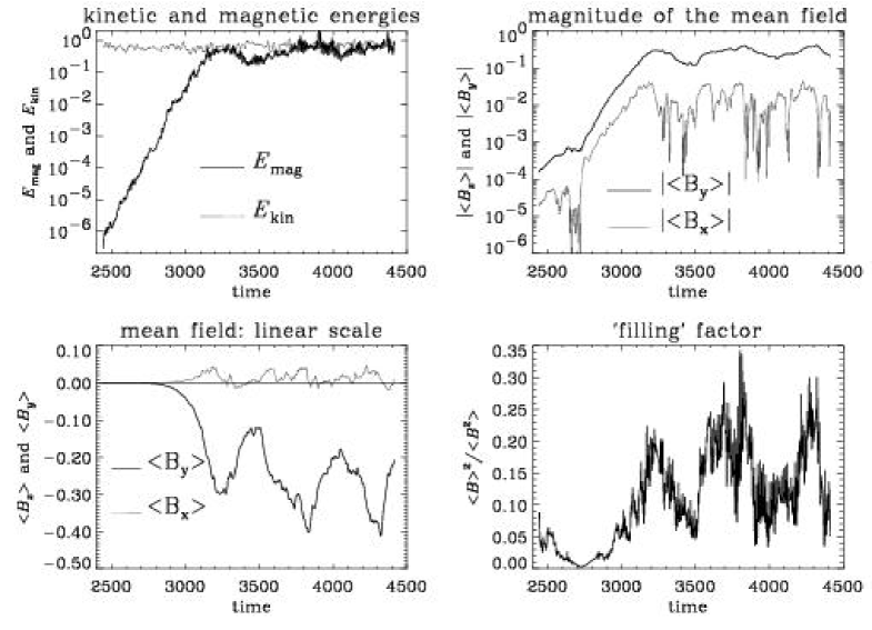
Figure 34: Evolution of several quantities for a convective dynamo model with shear: kinetic and magnetic energies (dotted and solid lines; first panel), mean latitudinal and toroidal fields (dotted and solid lines; second panel), mean magnetic field in a linear scale (third panel), and the filling factor (fourth panel). Energies and mean magnetic fields are given in units of the equipartition value, $B_{\rm eq}=4\pi\langle\mbox{\boldmath$u$}{}^{2}\rangle$.

In figure 34 we show the evolution of magnetic and kinetic energies as well as the magnitudes of the large scale field for a simulation of a convectively driven dynamo in the presence of large scale shear (Brandenburg, Nordlund, & Stein 2001). It turns out that the ratio of the magnetic energies in large scale fields relative to the total field, $\langle\mbox{\boldmath$B$}{}\rangle^{2}/\langle\mbox{\boldmath$B$}{}^{2}\rangle$, which is a measure of the filling factor of the magnetic field, is around 15% when the field has reached saturation, i.e. when the field growth has stopped. This is similar to the case of isotropic nonmirror-symmetric turbulence considered in § 7.1. On the average, however, the magnetic field is then directed into the negative $y$-direction (corresponding to the negative azimuthal direction in spherical geometry), but there is a weak and more noisy cross-stream field component directed in the positive $x$-direction (pointing north).

When the field has reached saturation, the mean field direction is approximately constant. Although the magnitude of this mean field fluctuates somewhat, the sign is always the same. Thus, this simulation shows no cycles, which are so characteristic of the solar dynamo. However, since those features, including the field geometry depend strongly on boundary condition and on the location of the boundary conditions, this disagreement is to be expected, and one would really need to resort to global simulations in spherical geometry.

7.11 Dynamics of the overshoot layer

Late-type stars with outer convection zones have an interface between the convection zone proper and the radiative interior. This leads to some additional dynamics that is important to include, especially in connection with the dynamo problem. This interface is the layer where magnetic flux can accumulate, i.e. not necessarily the layer where the dynamo operates; see the discussion in Brandenburg (1994). The accumulation is a consequence of turbulent pumping down the turbulence intensity gradient and the effect was seen clearly in video animations reported by Brandenburg & Tuominen (1991) and was analyzed in detail by Nordlund et al. (1992). Tobias et al. (1998) have studied the effect in isolation starting with an initial magnetic field distribution as opposed to a dynamo-generated field.

The flow dynamics changes drastically as one enters this overshoot layer. The stabilizing buoyancy effect provides a restoring force on a downward moving element, which can give rise to gravity waves that could be driven by individual plumes. This leads to a marked wavy pattern that can extend deep into the lower overshoot layer, as seen in figure 35 where we have plotted the vertical rms velocity as a function of depth and time. These waves extend a major fraction into the stably stratified layer beneath the convection zone, but are damped eventually. The typical period of such events is seen to be around 20 (in units of $\sqrt{d/g}$), where $d$ is the depth of the unstable (convective) layer. This is comparable with the mean Brunt-Väisälä frequency,

$$N_{\rm BV}^{2}=-\mbox{\boldmath$g$}{}\cdot\mbox{\boldmath$\nabla$}{}(s/c_{p}).$$ (185)

which is around 0.3 in the overshoot layer; see figure 36.

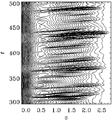
Figure 35: Space-time diagram of the vertical rms velocities for a nonmagnetic convection zone model of Brandenburg et al. (2001). Note the propagation of isolated plumes in more or less regular time intervals. Note also that the wavy pattern extends well into the convection zone proper ($0.5\leq z\leq 1$), and that the plumes appear to propagate at an approximately constant speed towards the bottom. This speed is around 0.1, which is comparable to the rms velocity in the runs.

Figure 36: Modulus of the Brunt-Väisälä frequency for a run with polytropic index $m=-0.9$ and a nondimensional input flux ${\cal F}_{\rm conv}=0.01$. The various curves are for different values of the radiative flux, but fixed nominal convective flux. Small values of ${\cal F}_{\rm rad}/{\cal F}_{\rm tot}$ are typical for the upper layers of the solar convection zone.

Technically the presence of a lower overshoot layer provides a formidable challenge, because there the dynamics is governed by the very slow thermal timescale. This can lead to problems if the properties of the upper surface layers change which could affect the entropy in deeper parts of the convection zone. This in turn will also affect the stratification in the rest of the radiative interior. Since this can only happen on a thermal timescale (there is no turbulence in these layers to speed things up) it takes very long before one arrives at a new statistically stable state. This problem is of course also encountered when starting with initial conditions that are derived under too unrealistic assumptions. There are essentially two different approaches to this: one either considers a toy model where dynamical and thermal timescales are artificially brought closer together or one adopts an implicit code which allows the use of somewhat longer timesteps. The former approach implies that one adopts input fluxes that exceed those in real stars, but the good news is that turbulent velocities and temperature fluctuations vary with changing flux in exactly the way that is expected from mixing length theory; see Brandenburg, Nordlund, & Stein (2001) for details.

8 Conclusions

Many phenomena in astrophysics show direct manifestations of turbulence. As in the case of accretion discs, without turbulence there would be no enhanced dissipation, no heating of the disc, and hence no emission. Magnetic fields are of major importance as is evidenced again by the example of accretion discs, where the turbulence is a direct consequence of the presence of magnetic fields (Balbus-Hawley instability). Although magnetic fields in discs could have primordial origin and could just have been compressed during their formation, it is also clear that discs are actually a favorable candidate for producing strong large scale magnetic fields, as shown by the local simulations discussed above.

Other bodies where strong dynamo action is possible are stars. Simulations of convection have shown that strong small scale magnetic fields are possible (Meneguzzi & Pouquet 1989, Nordlund et al. 1992, Brandenburg et al. 1996b, Cattaneo 1999), but if there is strong shear an intense large scale field can also emerge.

The use of nonconservative high order schemes has proved useful in all those applications. They are easy to implement and to modify, but they are also reasonably accurate. In this chapter we have illustrated the behavior of such schemes using various test problems. Using potential enthalpy and entropy as the main thermodynamic variables has a number of advantages, especially in connection with strongly stratified flows near a central object with a deep potential well, which is relevant to studying outflow phenomena. Contrary to common belief, high order schemes are not more vulnerable to Gibbs phenomena near discontinuities. Instead, in simple advection tests high order methods are able to produce smoother solutions with less viscosity, which is important for accurate modeling of turbulence.

In the last part of this chapter we have briefly mentioned some astrophysical applications of simulations using high order schemes where hydromagnetic turbulence played an important role. In the next few years we may expect a dramatic increase in the quality and predictive power of such simulations, as larger computers become available. Already now a number of very promising simulations are emerging. There is important work addressing the stability of astrophysical jets in three dimensions (Ouyed, Clarke, & Pudritz 2000). Also worthwhile mentioning are recent high resolution simulations by Hawley (2000) of three-dimensional accretion tori in global geometry. What remains to be done in this field is a proper connection between disc physics and the launching mechanism of jets. This would require incorporating proper thermodynamics allowing for radiative cooling and magnetic heating in particular. Global simulations would also be highly desirable to address the global stellar dynamo problem. It would be interesting to see how the dynamo works in fully convective stars, for example. This problem is in some ways simpler than the solar dynamo problem, because one does not need to worry about the lower overshoot layer where the relevant timescales are much longer than in the convection zone proper.

Acknowledgements:  I am indebted to Åke Nordlund for teaching me many of the methods and techniques that are reflected to some extend in the present work. I thank Wolfgang Dobler and Petri Käpylä for their careful reading of the manuscript and for pointing out a number of mistakes in the manuscript.

References

• Arber, T. D., Longbottom, A. W., Gerrard, C. L., & Milne, A. M.  2001  A staggered grid, Lagrangian-Eulerian remap code for 3D MHD simulations. J. Comp. Phys. 171, 151–181.

  Balbus, S. A. & Hawley, J. F.  1991  A powerful local shear instability in weakly magnetized disks. I. Linear analysis. Astrophys. J. 376, 214–222.

  Balsara, D., & Pouquet, A.  1999  The formation of large-scale structures in supersonic magnetohydrodynamic flows. Phys. Plasmas 6, 89–99.

  Benson, D. J.  1992  Computational methods in Lagrangian and Eulerian hydrocodes. Comp. Meth. Appl. Mech. Eng. 99, 235–394.

  Berger, M. A., & Ruzmaikin, A.  2000  Rate of helicity production by solar rotation. J. Geophys. Res. 105, 10481–10490.

  Biskamp, D.  1994  Cascade models for magnetohydrodynamic turbulence. Phys. Rev. E50, 2702–2711.

  Biskamp, D., & Müller, W.-C.  1999  Decay laws for three-dimensional magnetohydrodynamic turbulence. Phys. Rev. Lett. 83, 2195–2198.

  Bigazzi, A.  1999  Models of small-scale and large-scale dynamo action. PhD thesis, Università Degli Studi Dell’Aquila.

  Blackman, E. G., & Field, G. F.  2000  Constraints on the magnitude of $\alpha$ in dynamo theory. Astrophys. J. 534, 984–988.

  Blandford, R. D. & Payne, D. G.  1982  Hydromagnetic flows from accretion discs and the production of radio jets. Monthly Notices Roy. Astron. Soc. 199, 883–903.

  Brandenburg, A.  1992  Energy spectra in a model for convective turbulence. Phys. Rev. Lett. 69, 605–608.

  Brandenburg, A.  1994  Solar Dynamos: Computational Background. In Lectures on Solar and Planetary Dynamos (ed. M. R. E. Proctor & A. D. Gilbert), pp. 117–159. Cambridge University Press.

  Brandenburg, A.  1998  Disc Turbulence and Viscosity. In Theory of Black Hole Accretion Discs (ed. M. A. Abramowicz, G. Björnsson & J. E. Pringle), pp. 61–86. Cambridge University Press.

  Brandenburg, A.  1999  Helicity in large-scale dynamo simulations. In Magnetic Helicity in Space and Laboratory Plasmas (ed. M. R. Brown, R. C. Canfield, A. A. Pevtsov), pp. 65–73. Geophys. Monograph 111, American Geophysical Union, Florida.

  Brandenburg, A.  2000  Dynamo-generated turbulence and outflows from accretion discs. Phil. Trans. Roy. Soc. Lond. A 358, 759–776.

  Brandenburg, A.  2001a  Magnetic mysteries. Science 292, 2440–2441.

  Brandenburg, A.  2001b  The inverse cascade and nonlinear alpha-effect in simulations of isotropic helical hydromagnetic turbulence. Astrophys. J. 550, 824–840.

  Brandenburg, A., & Donner, K. J.  1997  The dependence of the dynamo alpha on vorticity. Monthly Notices Roy. Astron. Soc. 288, L29–L33.

  Brandenburg, A., & Schmitt, D.  1998  Simulations of an alpha-effect due to magnetic buoyancy. Astron. Astrophys. 338, L55–L58.

  Brandenburg, A., & Subramanian, K.  2000  Large scale dynamos with ambipolar diffusion nonlinearity. Astron. Astrophys. 361, L33–L36.

  Brandenburg, A., Tuominen, I.  1991  The solar dynamo. In The Sun and cool stars: activity, magnetism, dynamos, IAU Coll. 130 (ed. I. Tuominen, D. Moss & G. Rüdiger), pp. 223–233. Lecture Notes in Physics 380, Springer-Verlag.

  Brandenburg, A., Enqvist, K., Olesen, P.  1996  Large-scale magnetic fields from hydromagnetic turbulence in the very early universe. Phys. Rev. D 54, 1291–1300.

  Brandenburg, A., Nordlund, Å., & Stein, R. F.  2000  Astrophysical convection and dynamos. In Geophysical and Astrophysical Convection (ed. P. A. Fox & R. M. Kerr), pp. 85–105. Gordon and Breach Science Publishers.

  Brandenburg, A., Nordlund, Å., & Stein, R. F.  2001  “Simulation of a convective dynamo with imposed shear,” Astron. Astrophys. (to be submitted).

  Brandenburg, A., Nordlund, Å., Stein, R. F., & Torkelsson, U.  1995  Dynamo generated turbulence and large scale magnetic fields in a Keplerian shear flow. Astrophys. J. 446, 741–754.

  Brandenburg, A., Nordlund, Å., Stein, R. F., & Torkelsson, U.  1996a  The disk accretion rate for dynamo generated turbulence. Astrophys. J. Letters 458, L45–L48.

  Brandenburg, A., Jennings, R. L., Nordlund, Å., Rieutord, M., Stein, R. F., & Tuominen, I.  1996b  Magnetic structures in a dynamo simulation. J. Fluid Mech. 306, 325–352.

  Brandenburg, A., Dobler, W., Shukurov, A., & von Rekowski, B.  2000  “Pressure-driven outflow from a dynamo active disc,” Astron. Astrophys. (submitted). astro-ph/0003174

  Brandenburg, A., Chan, K. L., Nordlund, Å., Stein, R. F.  2001  “The effect of the radiative background flux in convection simulations,” Astron. Astrophys. (to be submitted).

  Brandenburg A., & Sarson, G. R.  2001  The effect of hyperdiffusivity on turbulent dynamos with helicity. http://www.nordita.dk/~brandenb/tmp/graeme/paper.ps.gz.

  Campbell, C. G.  1999  Launching of accretion disc winds along dynamo-generated magnetic fields. Monthly Notices Roy. Astron. Soc. 310, 1175–1184.

  Campbell, C. G.  2000  An accretion disc model with a magnetic wind and turbulent viscosity. Monthly Notices Roy. Astron. Soc. 317, 501–527.

  Canuto, C., Hussaini, M. Y., Quarteroni, A., & Zang, T. A.  1988  Spectral Methods in Fluid Dynamics. Springer, Berlin.

  Cattaneo, F.,  1999  On the origin of magnetic fields in the quiet photosphere. Astrophys. J. 515, L39–L42.

  Cattaneo, F., & Hughes, D. W.  1996  Nonlinear saturation of the turbulent alpha effect. Phys. Rev. E 54, R4532–R4535.

  Chan, K. L., & Sofia, S.  1986  Turbulent compressible convection in a deep atmosphere. II. Tests on the validity and limitation of the numerical approach. Astrophys. J. 307, 222–241.

  Chan, K. L., & Sofia, S.  1989  Turbulent compressible convection in a deep atmosphere. III. Results of three-dimensional computations. Astrophys. J. 336, 1022–1040.

  Choudhuri, A. R., Schüssler, M., & Dikpati, M.  1995  The solar dynamo with meridional circulation. Astron. Astrophys. 303, L29–L32.

  Collatz, L.  1966  The numerical treatment of differential equations. Springer-Verlag, New York., p. 164.

  Colella, P., & Woodward, P. R.  1984  The piecewise parabolic method (PPM) for gas-dynamical simulations. J. Comp. Phys. 54, 174–201.

  Dobler, W., Brandenburg, A., & Shukurov, A.  1999  Pressure-driven outflow and magneto-centrifugal wind from a dynamo active disc. In Plasma Turbulence and Energetic Particles in Astrophysics (ed. M. Ostrowski & R. Schlickeiser), pp. 347–352. Publ. Astron. Obs. Jagiellonian Univ., Cracow.

  Dodd, R. K., Eilbeck, J. C., Gibbon, J. D., & Morris, H. C.  1982  Solitons and nonlinear wave equations. Academic Press: London.

  Durney, B. R.  1995  On a Babcock-Leighton dynamo model with a deep-seated generating layer for the toroidal magnetic field. II. Solar Phys. 166, 231–260.

  Fox, P. A., Theobald, M. L., & Sofia, S.  1991  Compressible magnetic convection: formulation and two-dimensional models. Astrophys. J. 383, 860–881.

  Frank, J., King, A. R., & Raine, D. J.  1992  Accretion power in astrophysics. Cambridge: Cambridge Univ. Press.

  Frisch, U., Pouquet, A., Léorat, J., Mazure, A.  1975  Possibility of an inverse cascade of magnetic helicity in hydrodynamic turbulence. J. Fluid Mech. 68, 769–778.

  Galsgaard, K. & Nordlund, Å.  1996  Heating and activity of the solar corona: I. boundary shearing of an initially homogeneous magnetic-field. J. Geophys. Res. 101, 13445–13460.

  Galsgaard, K. & Nordlund, Å.  1997a  Heating and activity of the solar corona: II. Kink instability in a flux tube. J. Geophys. Res. 102, 219–230.

  Galsgaard, K. & Nordlund, Å.  1997b  Heating and activity of the solar corona: III. Dynamics of a low beta plasma with three-dimensional null points. J. Geophys. Res. 102, 231–248.

  Glatzmaier, G. A., & Roberts, P. H.  1995  A three-dimensional self-consistent computer simulation of a geomagnetic field reversal. Nature 377, 203–209.

  Glatzmaier, G. A., & Roberts, P. H.  1996  Rotation and magnetism of Earth’s inner core. Science 274, 1887–1891.

  Grauer, R., Marliani, C., & Germaschewski, K.  1998  Adaptive mesh refinement for singular solutions of the incompressible Euler equations. Phys. Rev. Lett. 80, 4177–4180.

  Greenhill, L. J., Gwinn, C. R., Schwartz, C., Moran, J. M., & Diamond, P. J.  1998  Coexisting conical bipolar and equatorial outflows from a high-mass protostar. Nature 396, 650–653.

  Hawley, J. F.  2000  Global magnetohydrodynamical simulations of accretion tori. Astrophys. J. 528, 462–479.

  Hawley, J. F., Gammie, C. F., & Balbus, S. A.  1995  Local three-dimensional magnetohydrodynamic simulations of accretion discs. Astrophys. J. 440, 742–763.

  Hawley, J. F., Gammie, C. F., & Balbus, S. A.  1996  Local three dimensional simulations of an accretion disk hydromagnetic dynamo. Astrophys. J. 464, 690–703.

  Hodapp, K.-W. & Ladd, E. F.  1995  Bipolar jets from extremely young stars observed in molecular hydrogen emission. Astrophys. J. 453, 715–720.

  Ji, H., Prager, S. C., Almagri, A. F., Sarff, J. S., & Toyama, H.  1996  Measurement of the dynamo effect in a plasma. Phys. Plasmas 3, 1935–1942.

  Kerr, R. M., & Brandenburg, A.  1999  Evidence for a singularity in ideal magnetohydrodynamics: implications for fast reconnection. Phys. Rev. Lett. 83, 1155–1158.

  Kleeorin, N. I, Moss, D., Rogachevskii, I., & Sokoloff, D.  2000  Helicity balance and steady-state strength of the dynamo generated galactic magnetic field. Astron. Astrophys. 361, L5–L8.

  Korpi, M. J., Brandenburg, A., Shukurov, A., Tuominen, I., & Nordlund, Å.  1999  A supernova regulated interstellar medium: simulations of the turbulent multiphase medium. Astrophys. J. Letters 514, L99–L102.

  Lele, S. K.  1992  Compact finite difference schemes with spectral-like resolution. J. Comp. Phys. 103, 16–42.

  LeVeque, R. J., Mihalas, D., Dorfi, E. A., & Müller, E.  1998  Computational methods for astrophysical fluid flow. Springer, Berlin.

  Lohse, D., & Müller-Groeling, A.  1995  Bottleneck effects in turbulence: Scaling phenomena in r versus p space. Phys. Rev. Lett. 74, 1747–1750.

  Mac Low, M.-M., Klessen, R. S., & Burkert, A.  1998  Kinetic energy decay rates of supersonic and super-Alfvénic turbulence in star-forming clouds. Phys. Rev. Lett. 80, 2754–2757.

  Meneguzzi, M., & Pouquet, A.  1989  Turbulent dynamos driven by convection. J. Fluid Mech. 205, 297–312.

  Nordlund, Å.  1982  Numerical Simulations of the Solar Granulation I. Basic Equations and Methods. Astron. Astrophys. 107, 1–10.

  Nordlund, Å.  1985  Solar convection. Solar Phys. 100, 209–235.

  Nordlund, Å., & Galsgaard, K.  1995  A 3D MHD code for Parallel Computers. http://www.astro.ku.dk/~aake/NumericalAstro/papers/kg/mhd.ps.gz.

  Nordlund, Å., & Stein, R. F.  1990  3-D Simulations of Solar and Stellar Convection and Magnetoconvection. Comput. Phys. Commun. 59, 119–125.

  Nordlund, Å., Galsgaard, K., & Stein, R. F.  1994  Magnetoconvection and Magnetoturbulence. In Solar surface magnetic fields (ed. R. J. Rutten & C. J. Schrijver), pp. 471–498. NATO ASI Series, Vol. 433.

  Nordlund, Å., Brandenburg, A., Jennings, R. L., Rieutord, M., Ruokolainen, J., Stein, R. F., & Tuominen, I.  1992  Dynamo action in stratified convection with overshoot. Astrophys. J. 392, 647–652.

  Ouyed, R., Pudritz, R. E. & Stone, J. M.  1997  Episodic jets from black holes and protostars. Nature 385, 409–414.

  Ouyed, R., & Pudritz, R. E.  1997a  Numerical simulations of astrophysical jets from keplerian discs. I. Stationary models. Astrophys. J. 482, 712–732.

  Ouyed, R., & Pudritz, R. E.  1997b  Numerical simulations of astrophysical jets from keplerian discs. II. Episodic outflows. Astrophys. J. 484, 794–809.

  Ouyed, R., & Pudritz, R. E.  1999  Numerical simulations of astrophysical jets from keplerian discs. III. The effects of mass loading. Monthly Notices Roy. Astron. Soc. 309, 233–244.

  Ouyed, R., Clarke, D. A. & Pudritz, R. E.: 2000, “3-Dimensional simulations of astrophysical jets from keplerian accretion Disks I: stability issues,” Astrophys. J. (in press, scheduled for the

  issue)Padoan, P., Nordlund, Å., & Jones, B. J. T.  1997  The universality of the stellar mass function. Astrophys. J. 288, 145–152.

  Padoan, P., & Nordlund, Å.  1999  A super-Alfv nic model of dark clouds. Astrophys. J. 526, 279–294.

  Passot, T., & Pouquet, A.  1987  Numerical simulation of compressible homogeneous flows in the turbulent regime. J. Fluid Mech. 181, 441–466.

  Pelletier, G., & Pudritz, R. E.  1992  Hydromagnetic disk winds in young stellar objects and active galactic nuclei. Astrophys. J. 394, 117–138.

  Peterkin, R. E., Frese, M. H., & Sovinec, C. R.  1998  Transport of magnetic flux in an arbitrary coordinate ALE code. J. Comp. Phys. 140, 148–171.

  Porter, D. H., Pouquet A., & Woodward, P. R.  1992  Three-dimensional supersonic homogeneous turbulence: a numerical study. Phys. Rev. Lett. 68, 3156–3159.

  Porter, D. H., Pouquet A., & Woodward, P. R.  1994  Kolmogorov-like spectra in decaying 2-dimensional supersonic flows. Phys. Fluids 6, 2133–2142.

  Pouquet, A., Frisch, U., Léorat, J.  1976  Strong MHD helical turbulence and the nonlinear dynamo effect. J. Fluid Mech. 77, 321–354.

  Rast, M. P., Nordlund, Å., Stein, R.F., & Toomre, J.  1993  Ionization effects in three–dimensional granulation simulations. Astrophys. J. Letters 408, L53–L56.

  Rast, M. P., & Toomre, J.  1993a  Compressible convection with ionization. I. Stability, flow asymmetries, and energy transport. Astrophys. J. 419, 224–239.

  Rast, M. P., & Toomre, J.  1993b  Compressible convection with ionization. II. Thermal boundary-layer instability. Astrophys. J. 419, 240–254.

  Rekowski, M. v., Rüdiger, G., & Elstner, D.  2000  Structure and magnetic configurations of accretion disk-dynamo models. Astron. Astrophys. 353, 813–822.

  Roettiger, K., Stone, J. M., & Burns, J. O.  1999  Magnetic field evolution in merging clusters of galaxies. Astrophys. J. 518, 594–602.

  Rögnvaldsson, Ö. E., Nordlund, Å., & Sommer-Larsen, J.  2001  Cooling flows and disk galaxy formation. preprint.

  Rogallo, R. S.  1981  Numerical experiments in homogeneous turbulence. NASA Tech. Memo. 81315.

  Sánchez-Salcedo, F. J., & Brandenburg, A.  1999  Deceleration by dynamical friction in a gaseous medium. Astrophys. J. Letters 522, L35–L38.

  Sánchez-Salcedo, F. J., & Brandenburg, A.  2001  Dynamical friction of bodies orbiting in a gaseous sphere. Monthly Notices Roy. Astron. Soc. 322, 67–78.

  Sod, G. A.  1978  A survey of several finite difference methods for systems of nonlinear hyperbolic conservation laws. J. Comp. Phys. 27, 1–31.

  Stanescu, D. & Habashi, W. G.  1998  $2N$-storage low dissipation and dispersion Runge-Kutta schemes for computational acoustics. J. Comp. Phys. 143, 674–681.

  Steffen, M., Ludwig, H.-G., & Krüß, A.  1989  A numerical study of solar granular convection in cells of different horizontal dimensions. Astron. Astrophys. 123, 371–382.

  Stein, R.F., & Nordlund, Å.  1989  Topology of convection beneath the solar surface. Astrophys. J. Letters 342, L95–L98.

  Stein, R.F., & Nordlund, Å.  1998  Simulations of solar granulation. I. General properties. Astrophys. J. 499, 914–933.

  Stone, J. M., Norman, M.  1992a  ZEUS-2D: A radiation magnetohydrodynamics code for astrophysical flows in two space dimensions: I. The hydrodynamic algorithms and tests. Astrophys. J. 80, 753–790

  Stone, J. M., Norman, M.  1992b  ZEUS-2D: A radiation magnetohydrodynamics code for astrophysical flows in two space dimensions: II. The magnetohydrodynamic algorithms and tests. Astrophys. J. 80, 791–818

  Stone, J. M., Hawley, J. F., Gammie, C. F., & Balbus, S. A.  1996  Three dimensional magnetohydrodynamical simulations of vertically stratified accretion disks. Astrophys. J. 463, 656–673.

  Stewart, J. M.  1975  The hydrodynamics of accretions discs I: Stability. Astron. Astrophys. 42, 95–101.

  Suzuki, E. & Toh, S.  1995  Entropy cascade and temporal intermittency in a shell model for convective turbulence. Phys. Rev. E 51, 5628–5635.

  Thelen, J.-C.  2000  A mean electromotive force induced by magnetic buoyancy instabilities. Monthly Notices Roy. Astron. Soc. 315, 155–164.

  Tobias, S. M., Brummell, N. H., Clune, T. L., & Toomre, J.  1998  Pumping of magnetic fields by turbulent penetrative convection. Astrophys. J. Letters 502, L177–L177.

  Toh, S., & Iima, M.  2000  Dynamical aspect of entropy transfer in free convection turbulence. Phys. Rev. E 61, 2626–2639.

  Urpin, V., & Brandenburg, A.  1998  Magnetic and vertical shear instabilities in accretion discs. Monthly Notices Roy. Astron. Soc. 294, 399–406.

  Vainshtein, S. I., & Cattaneo, F.  1992  Nonlinear restrictions on dynamo action. Astrophys. J. 393, 165–171.

  Vishniac, E. T., & Brandenburg, A.  1997  An incoherent $\alpha-\Omega$ dynamo in accretion disks. Astrophys. J. 475, 263–274.

  Völk, H. J. & Atoyan, A. M.  1999  Clusters of galaxies: magnetic fields and nonthermal emission. Astroparticle Phys. 11, 73–82.

  Williamson, J. H.  1980  Low-storage Runge-Kutta schemes. J. Comp. Phys. 35, 48–.

  Ziegler, U., & Rüdiger, G.  2000  Angular momentum transport and dynamo-effect in stratified, weakly magnetic disks. Astron. Astrophys. 356, 1141–1148.

Appendix

Appendix A Centered, onesided and semi-onesided derivatives

In § 3 we gave the centered finite difference formulae for schemes of different order. Here we first describe the method for determining the finite difference formulae for second order, but the generalization to higher order is straightforward. We also give the corresponding expressions for one-sided and semi-onesided finite difference formulae.

We want to write the derivative $f^{\prime}(x)$ at the point $x_{i}$ as

$$f^{\prime}_{i}=a_{-1}f_{i-1}+a_{0}f_{0}+a_{1}f_{1},$$ (186)

where $f^{\prime}_{i}=f^{\prime}(x_{i})$, $f_{i-1}=f(x_{i}-\delta x)$, and $f_{i+1}=f(x_{i}+\delta x)$. To determine the coefficients $a_{-1}$, $a_{0}$ and $a_{1}$ we expand $f(x)$ up to second order

$$f(x)=c_{0}+c_{1}x+c_{2}x^{2}.$$ (187)

The first derivative is then

$$f^{\prime}(x)=c_{1}+2c_{2}x.$$ (188)

In particular, the value at $x=0$ is just $f^{\prime}(0)=c_{1}$. Likewise, we have $f^{\prime\prime}(0)=2c_{2}$ To determine all coefficients we make use of our knowledge at the neighboring points around $x_{i}$, i.e. we use the function values $f(x_{i}-\delta x)\equiv f_{i-1}$, $f(x_{i})\equiv f_{i}$, and $f(x_{i}+\delta x)\equiv f_{i+1}$, so we have

$$f_{i-1} = c_{0}+c_{1}(-\delta x)+c_{2}(-\delta x)^{2},$$ (189)

$$f_{i} = c_{0},$$ (190)

$$f_{i+1} = c_{0}+c_{1}(+\delta x)+c_{2}(+\delta x)^{2}.$$ (191)

This can be written in matrix form

$$\pmatrix{f_{i-1}\cr f_{i}\cr f_{i+1}}=\pmatrix{(-1)^{0}&(-1)^{1}&(-1)^{2}\cr 0^{0}&0^{1}&0^{2}\cr 1^{0}&1^{1}&1^{2}\cr}\pmatrix{c_{0}\cr c_{1}\delta x\cr c_{2}\delta x^{2}}$$ (192)

(where $(-1)^{0}=0^{0}=1^{0}=1$), or

$$\mbox{\boldmath$f$}{}=\mbox{\boldmath$M$}{}\mbox{\boldmath$c$}{},$$ (193)

and so we obtain the coefficients as

$$\mbox{\boldmath$c$}{}=\mbox{\boldmath$M$}{}^{-1}\mbox{\boldmath$f$}{}.$$ (194)

To calculate $f^{\prime}$ we need the value of $c_{1}$, see eq. (188), and so the coefficients $a_{n}$ needed to express the derivative are $a_{-1}=(\mbox{\boldmath$M$}{}^{-1})_{10}$, $a_{0}=(\mbox{\boldmath$M$}{}^{-1})_{11}$, and $a_{1}=(\mbox{\boldmath$M$}{}^{-1})_{12}$, i.e. all points of the inverted matrix in the second row. The resulting formula for $f^{\prime}_{i}$ is well-known,

$$f^{\prime}_{i}=(-f_{i-1}+f_{i+1})/(2\delta x).$$ (195)

The corresponding result for the second derivative is

$$f^{\prime\prime}_{i}=(f_{i-1}-2f_{i}+f_{i+1})/(\delta x^{2}).$$ (196)

On the boundaries we have to calculate for derivative using only points inside the domain, which is explained in the next subsection for second order accuracy, but again the generalization to higher order is straightforward and only the results will be listed.

A.1 One-sided 2nd order derivatives

Again, we want to write the derivative $f^{\prime}(x)$ as

$$f^{\prime}_{i}=a_{0}f_{0}+a_{1}f_{1}+a_{2}f_{2},$$ (197)

but now

$$\pmatrix{f_{i}\cr f_{i+1}\cr f_{i+2}}=\pmatrix{0^{0}&0^{1}&0^{2}\cr 1^{0}&1^{1}&1^{2}\cr 2^{0}&2^{1}&2^{2}}\pmatrix{c_{0}\cr c_{1}\delta x\cr c_{2}\delta x^{2}}$$ (198)

Thus, one arrives at

$$f^{\prime}_{i}=(-3f_{i}+4f_{i+1}-f_{i+2})/(2\delta x).$$ (199)

Correspondingly, for the second derivative we have

$$f^{\prime\prime}_{i}=(2f_{i}-5f_{i+1}+4f_{i+2}-f_{i+3})/\delta x^{2}.$$ (200)

A.2 4th order derivatives

First derivatives

$$f^{\prime}_{i}=(f_{i-2}-8f_{i-1}+8f_{i+1}-f_{i+2})/(12\delta x)$$ (201)

$$f^{\prime}_{i}=(-3f_{i-1}-10f_{i}+18f_{i+1}-6f_{i+2}+f_{i+3})/(12\delta x)$$ (202)

$$f^{\prime}_{i}=(-25f_{i}+48f_{i+1}-36f_{i+2}+16f_{i+3}-3f_{i+4})/(12\delta x)$$ (203)

Second derivatives

$$f^{\prime\prime}_{i}=(-f_{i-2}+16f_{i-1}-30f_{i}+16f_{i+1}-f_{i+2})/(12\delta x^{2})$$ (204)

$$f^{\prime\prime}_{i}=(11f_{i-1}-20f_{i}+6f_{i+1}+4f_{i+2}-f_{i+3})/(12\delta x^{2})$$ (205)

$$f^{\prime\prime}_{i}=(35f_{i}-104f_{i+1}+114f_{i+2}-56f_{i+3}+11f_{i+4})/(12\delta x^{2})$$ (206)

A.3 6th order derivatives

First derivatives

$$f^{\prime}_{i}=(-f_{i-3}+9f_{i-2}-45f_{i-1}+45f_{i+1}-9f_{i+2}+f_{i+3})/(60\delta x)$$ (207)

$$f^{\prime}_{i}=(2f_{i-2}-24f_{i-1}-35f_{i}+80f_{i+1}-30f_{i+2}+8f_{i+3}-f_{i+4})/(60\delta x)$$ (208)

$$f^{\prime}_{i}=(-10f_{i-1}-77f_{i}+150f_{i+1}-100f_{i+2}+50f_{i+3}-15f_{i+4}+2f_{i+5})/(60\delta x)$$ (209)

$$f^{\prime}_{i}=(-147f_{i}+360f_{i+1}-450f_{i+2}+400f_{i+3}-225f_{i+4}+72f_{i+5}-10f_{i+6})/(60\delta x)$$ (210)

Second derivatives

$$f^{\prime\prime}_{i}=(2f_{i-3}-27f_{i-2}+270f_{i-1}-490f_{i}+270f_{i+1}-27f_{i+2}+2f_{i+3})/(180\delta x^{2})$$ (211)

$$f^{\prime\prime}_{i}=(-13f_{i-2}+228f_{i-1}-420f_{i}+200f_{i+1}+15f_{i+2}-12f_{i+3}+2f_{i+4})/(180\delta x^{2})$$ (212)

$$f^{\prime\prime}_{i}=(137f_{i-1}-147f_{i}-255f_{i+1}+470f_{i+2}-285f_{i+3}+93f_{i+4}-13f_{i+5})/(180\delta x^{2})$$ (213)

$$f^{\prime\prime}_{i}=\left(812f_{i}-3132f_{i+1}+5265f_{i+2}-5080f_{i+3}+2970f_{i+4}-972f_{i+5}+137f_{i+6}\right)/(180\delta x^{2})$$ (214)

Appendix B The $2N$-RK3 scheme

If $N$ is the number of variables to be updated from one timestep to the next, the $2N$-schemes require only $2\times N$ variables to be stored in memory at any time. This is better than for the standard Runge-Kutta schemes. The general iteration formula is

$$w_{i}=\alpha_{i}w_{i-1}+hF(t_{i-1},u_{i-1}),\quad u_{i}=u_{i-1}+\beta_{i}w_{i}.$$ (215)

For a third order scheme we have $i=1,...,3$. In order to advance the variable $u$ from $u^{(n)}$ at time $t^{(n)}$ to $u^{(n+1)}$ at time $t^{(n+1)}=t^{(n)}+h$ we set in eq. (215)

$$u_{0}=u^{(n)}\quad\mbox{and}\quad u_{3}=u^{(n+1)},$$ (216)

with $u_{1}$ and $u_{2}$ being intermediate steps. In order to be able to calculate the first step, $i=1$, for which no $w_{i-1}\equiv w_{0}$ exists, we have to require $\alpha_{1}=0$. Thus, we are left with 5 unknowns, $\alpha_{2}$, $\alpha_{3}$, $\beta_{1}$, $\beta_{2}$, and $\beta_{3}$. We write down eq. (215) in explicit form for $i=1,...,3$,

$$w_{1}=hF(t_{0},u_{0}),\quad u_{1}=u_{0}+\beta_{1}w_{1}.$$ (217)

$$w_{2}=\alpha_{2}w_{1}+hF(t_{1},u_{1}),\quad u_{2}=u_{1}+\beta_{2}w_{2}.$$ (218)

$$w_{3}=\alpha_{3}w_{2}+hF(t_{2},u_{2}),\quad u_{3}=u_{2}+\beta_{3}w_{3}.$$ (219)

Written in explicit form, we have for $i=1$

$$u_{1}=u_{0}+\beta_{1}hF(t_{0},u_{0}).$$ (220)

The $i=2$ step yields

$$w_{2}=\alpha_{2}hF(t_{0},u_{0})+hF(t_{1},u_{1}),$$ (221)

$$u_{2}=u_{0}+h\left[(\beta_{1}+\beta_{2}\alpha_{2})F(t_{0},u_{0})+\beta_{2}F(t_{1},u_{1})\right].$$ (222)

and the $i=3$ step gives

$$w_{3}=h\left[\alpha_{2}\alpha_{3}F(t_{0},u_{0})+\alpha_{3}F(t_{1},u_{1})+F(t_{2},u_{2})\right]$$ (223)

$$u_{3}=u_{0}+\left[\beta_{1}+\alpha_{2}(\beta_{2}+\alpha_{3}\beta_{3})\right]hF(t_{0},u_{0})+(\beta_{2}+\beta_{3}\alpha_{3})hF(t_{1},u_{1})+\beta_{3}hF(t_{2},u_{2}).$$ (224)

The corresponding times can be calculated by putting $F=1$. This yields

$$t_{1}=t_{0}+\beta_{1}h,$$ (225)

$$t_{2}=t_{0}+h\left[\beta_{1}+\beta_{2}(1+\alpha_{2})\right],$$ (226)

$$t_{3}=t_{0}+h\left[\beta_{1}+\beta_{3}+(1+\alpha_{2})(\beta_{2}+\alpha_{3}\beta_{3})\right].$$ (227)

The last expression can also be written in the form

$$t_{3}=t_{0}+h\left\{\beta_{1}+\beta_{2}(1+\alpha_{2})+\beta_{3}\left[1+(1+\alpha_{2})\alpha_{3})\right]\right\}$$ (228)

Next we need to determine the conditions that the scheme is indeed of third order. This can be done by considering the differential equation

$${\rm d}{}u/{\rm d}{}t=u,\quad u(0)=u_{0},$$ (229)

for $u=u(t)$, where $u_{0}$ is the initial value of $u$. The exact solution of eq. (229) is $u_{0}e^{t}$. Its Taylor expansion for $t=t_{0}+h$ is

$$u(t_{0}+h)=u_{0}[1+h+{\textstyle{1\over 2}}h^{2}+{\textstyle{1\over 6}}h^{3}+...].$$ (230)

The solution based on eq. (224) is

$$u_{3}=u_{0}+\left[\beta_{1}+\alpha_{2}(\beta_{2}+\alpha_{3}\beta_{3})\right]hu_{0}+(\beta_{2}+\alpha_{3}\beta_{3})hu_{1}+\beta_{3}hu_{2}$$ (231)

In order to compare with eq. (230) we need the explicit expressions for $u_{1}$ and $u_{2}$, which are

$$u_{1}=(1+h\beta_{1})u_{0}$$ (232)

$$u_{2}=\left\{1+h\left[\beta_{1}+(1+\alpha_{2})\beta_{2}\right]+h^{2}\beta_{1}\beta_{2}\right\}u_{0}.$$ (233)

and so we can write

$$u_{3}=u_{0}+\gamma_{1}h+\gamma_{2}h^{2}+\gamma_{3}h^{3}$$ (234)

with

$$\gamma_{1}=\beta_{1}+\beta_{3}+(1+\alpha_{2})(\beta_{2}+\alpha_{3}\beta_{3})$$ (235) $$\gamma_{2}=\beta_{1}\beta_{2}+\beta_{3}[\beta_{2}(1+\alpha_{2})+\beta_{1}(1+\alpha_{3})]$$ (236) $$\gamma_{3}=\beta_{1}\beta_{2}\beta_{3}$$ (237) In order for the scheme to be third order we have to require $\gamma_{1}=1$, $\gamma_{2}=1/2$, and $\gamma_{3}=1/6$; see eq. (230). Thus, we have now three equations for five unknowns. We now have to come up with two more equations to solve for the five unknowns.

If we assume that the intermediate timesteps are evaluated in equidistant time intervals, we have to require that the time increments in eqs. (225) and (226) are $1/3$ and $2/3$, respectively. This yields

$$\beta_{1}=\beta_{2}(1+\alpha_{2})=1/3,$$ (238)

with two particular solutions

$$\left\{\begin{array}[]{l}\alpha_{2}=-2/3,\quad\alpha_{3}=-1,\quad\beta_{1}=1/3,\quad\beta_{2}=1,\quad\beta_{3}=1/2,\\ \alpha_{2}=-1/3,\quad\alpha_{3}=-1,\quad\beta_{1}=1/3,\quad\beta_{2}=1/2,\quad\beta_{3}=1.\end{array}\right.$$ (241)

These are in fact the simplest $2N$-RK3 schemes that also lead to comparatively small residual errors.

Alternatively, one can move the times closer to the end time of the time step and evaluate the right hand side at times $t_{1}-t_{0}={1\over 2}h$ and $t_{2}-t_{0}=h$. This gives the particular solution

$$\alpha_{2}=-1/4,\quad\alpha_{3}=-4/3,\quad\beta_{1}=1/2,\quad\beta_{2}=2/3,\quad\beta_{3}=1/2.$$ (242)

Again, there could be other solutions.

Another possibility is to require that the inhomogeneous equation

$${\rm d}{}u/{\rm d}{}t=t^{n},\quad u(0)=0,$$ (243)

is solved exactly up to some $n$. The exact solutions for $t=h$ are $u={\textstyle{1\over 2}}h^{2}$ for $n=1$ and $u={\textstyle{1\over 3}}h^{3}$ for $n=2$.

The case $n=0$ was already considered in eqs. (225)–(227). For $n=1$ we have $F(t_{1},u_{1})={\textstyle{1\over 3}}h$ and $F(t_{2},u_{2})={\textstyle{2\over 3}}h$, so eq. (224) gives

$$u_{3}=u_{0}+(\beta_{2}+\beta_{3}\alpha_{3}){\textstyle{1\over 3}}h^{2}+\beta_{3}{\textstyle{2\over 3}}h^{2},$$ (244)

or

$$u_{3}=u_{0}+{\textstyle{1\over 3}}[\beta_{2}+\beta_{3}(\alpha_{3}+2)]h^{2}.$$ (245)

Comparing with the exact solution this yields the additional equation

$$\beta_{2}+\beta_{3}(\alpha_{3}+2)={\textstyle{3\over 2}}.$$ (246)

For $n=2$ we have $F(t_{1},u_{1})={1\over 9}h^{2}$ and $F(t_{2},u_{2})={4\over 9}h^{2}$, so eq. (224) gives

$$u_{3}=u_{0}+(\beta_{2}+\beta_{3}\alpha_{3}){\textstyle{1\over 9}}h^{3}+\beta_{3}{\textstyle{4\over 9}}h^{3},$$ (247)

or

$$u_{3}=u_{0}+{\textstyle{1\over 9}}[\beta_{2}+\beta_{3}(\alpha_{3}+4)]h^{3}.$$ (248)

Again, comparing with the exact solution one obtains

$$\beta_{2}+\beta_{3}(\alpha_{3}+4)=3.$$ (249)

This gives the solution

$$\alpha_{2}=-17/32,\quad\alpha_{3}=-32/27,\quad\beta_{1}=1/4,\quad\beta_{2}=8/9,\quad\beta_{3}=3/4,$$ (250)

which implies that the right hand sides are evaluated at the times $t_{1}-t_{0}={1\over 4}h$ and $t_{2}-t_{0}={2\over 3}h$. In tables LABEL:Ttab_2N-RK3 and LABEL:Ttab_2N-RK3-err this scheme is referred to as “inhomogeneous”.

Yet another idea (W. Dobler, private communication) is to obtain the additional two equations by requiring that the quadratic differential equation ${\rm d}{}u/{\rm d}{}t=u^{2}$ with $u_{0}=1$ is solved exactly. The solution is $u=(1-t)^{-1}$, of which we only need the expansion up to $h^{2}$, so we have $u_{3}\approx 1+h+h^{2}$. Again, we use eq. (224), but now with $F=u^{2}$,

$$u_{3}=1+\left[\beta_{1}+\alpha_{2}(\beta_{2}+\alpha_{3}\beta_{3})\right]h+(\beta_{2}+\alpha_{3}\beta_{3})hu_{1}^{2}+\beta_{3}hu_{2}^{2}.$$ (251)

We need $u_{1}^{2}$ and $u_{2}^{2}$ only up to the term linear in $h$. Using eqs. (232) and (233) we have

$$u_{1}^{2}=1+2\beta_{1}h+{\cal O}(h^{2}),\quad u_{2}^{2}=1+2\left[\beta_{1}+(1+\alpha_{2})\beta_{2}\right]h+{\cal O}(h^{2}).$$ (252)

Inserting this in eq. (251) yields

$$u_{3}=1+\delta_{1}h+\delta_{2}h^{2}+{\cal O}(h^{3}),$$ (253)

with

$$\delta_{1}=\beta_{1}+\alpha_{2}(\beta_{2}+\alpha_{3}\beta_{3})+(\beta_{2}+\alpha_{3}\beta_{3})+\beta_{3}$$ (254)

and

$$\delta_{2}=2\beta_{1}(\beta_{2}+\alpha_{3}\beta_{3})+2\beta_{3}\left[\beta_{1}+(1+\alpha_{2})\beta_{2}\right].$$ (255)

Thus, the two additional equations are

$$\beta_{1}+(1+\alpha_{2})(\beta_{2}+\alpha_{3}\beta_{3})+\beta_{3}=1,$$ (256)

$$\beta_{1}\left[\beta_{2}+(1+\alpha_{3})\beta_{3}\right]+(1+\alpha_{2})\beta_{2}=1/2.$$ (257)

The numerical solution is

$$\alpha_{2}=-0.36726297,\quad\alpha_{3}=-1.0278248,\quad\beta_{1}=0.30842796,\quad\beta_{2}=0.54037434,\quad\beta_{3}=1.$$ (258)

which implies that the right hand sides are evaluated at the times $t_{1}-t_{0}=0.308h$ and $t_{2}-t_{0}=0.650h$. In tables LABEL:Ttab_2N-RK3 and LABEL:Ttab_2N-RK3-err this scheme is referred to as “quadratic”.

Appendix C Derivation of the jacobian for transformation on a sphere

Here we give the explicit derivation of eqs. (79) and (80). We first use the transformation in the form

$$x=\tilde{x}^{2}/\tilde{r},\quad y=\tilde{x}\tilde{y}/\tilde{r},\quad\mbox{if $\tilde{x}\geq\tilde{y}$},$$ (259)

$$x=\tilde{x}\tilde{y}/\tilde{r},\quad y=\tilde{y}^{2}/\tilde{r},\quad\mbox{if $\tilde{x}\leq\tilde{y}$}.$$ (260)

To obtain the jacobian we differentiate with respect to $x$, so

$$1=2{\partial\ln\tilde{x}\over\partial\ln x}-{\partial\ln\tilde{r}\over\partial\ln x},\quad 0={\partial\ln\tilde{x}\over\partial\ln x}+{\partial\ln\tilde{y}\over\partial\ln x}-{\partial\ln\tilde{r}\over\partial\ln x},\quad\mbox{if $\tilde{x}\geq\tilde{y}$},$$ (261)

$$1={\partial\ln\tilde{x}\over\partial\ln x}+{\partial\ln\tilde{y}\over\partial\ln x}-{\partial\ln\tilde{r}\over\partial\ln x},\quad 0=2{\partial\ln\tilde{y}\over\partial\ln x}-{\partial\ln\tilde{r}\over\partial\ln x},\quad\mbox{if $\tilde{x}\leq\tilde{y}$}.$$ (262)

We now differentiate with respect to $y$,

$$0=2{\partial\ln\tilde{x}\over\partial\ln y}-{\partial\ln\tilde{r}\over\partial\ln y},\quad 1={\partial\ln\tilde{x}\over\partial\ln y}+{\partial\ln\tilde{y}\over\partial\ln y}-{\partial\ln\tilde{r}\over\partial\ln y},\quad\mbox{if $\tilde{x}\geq\tilde{y}$},$$ (263)

$$0={\partial\ln\tilde{x}\over\partial\ln y}+{\partial\ln\tilde{y}\over\partial\ln y}-{\partial\ln\tilde{r}\over\partial\ln y},\quad 1=2{\partial\ln\tilde{y}\over\partial\ln y}-{\partial\ln\tilde{r}\over\partial\ln y},\quad\mbox{if $\tilde{x}\leq\tilde{y}$}.$$ (264)

The derivatives of $\tilde{r}$ can be written as

$${\partial\ln\tilde{r}\over\partial\ln x}=\left({\tilde{x}\over\tilde{r}}\right)^{2}{\partial\ln\tilde{x}\over\partial\ln x}+\left({\tilde{y}\over\tilde{r}}\right)^{2}{\partial\ln\tilde{y}\over\partial\ln x},$$ (265)

$${\partial\ln\tilde{r}\over\partial\ln y}=\left({\tilde{x}\over\tilde{r}}\right)^{2}{\partial\ln\tilde{x}\over\partial\ln y}+\left({\tilde{y}\over\tilde{r}}\right)^{2}{\partial\ln\tilde{y}\over\partial\ln y}.$$ (266)

In all cases we have

$${x\over y}={\tilde{x}\over\tilde{y}},$$ (267)

so

$$+1={\partial\ln\tilde{x}\over\partial\ln x}-{\partial\ln\tilde{y}\over\partial\ln x},$$ (268)

$$-1={\partial\ln\tilde{x}\over\partial\ln y}-{\partial\ln\tilde{y}\over\partial\ln y},$$ (269)

and so

$$1=2{\partial\ln\tilde{x}\over\partial\ln x}-\left({\tilde{x}\over\tilde{r}}\right)^{2}{\partial\ln\tilde{x}\over\partial\ln x}-\left({\tilde{y}\over\tilde{r}}\right)^{2}\left({\partial\ln\tilde{x}\over\partial\ln x}-1\right),\quad\mbox{if $\tilde{x}\geq\tilde{y}$},$$ (270)

$$0={\partial\ln\tilde{x}\over\partial\ln x}+{\partial\ln\tilde{y}\over\partial\ln x}-\left({\tilde{x}\over\tilde{r}}\right)^{2}{\partial\ln\tilde{x}\over\partial\ln x}-\left({\tilde{y}\over\tilde{r}}\right)^{2}\left({\partial\ln\tilde{x}\over\partial\ln x}-1\right),\quad\mbox{if $\tilde{x}\geq\tilde{y}$},$$ (271)

so

$$1={\partial\ln\tilde{x}\over\partial\ln x}+\left({\tilde{y}\over\tilde{r}}\right)^{2},\quad\mbox{if $\tilde{x}\geq\tilde{y}$},$$ (272)

and so

$${\partial\ln\tilde{x}\over\partial\ln x}=1-\left({\tilde{y}\over\tilde{r}}\right)^{2},\quad{\partial\ln\tilde{y}\over\partial\ln x}=-\left({\tilde{y}\over\tilde{r}}\right)^{2},\quad\mbox{if $\tilde{x}\geq\tilde{y}$},$$ (273)

and correspondingly

$$1={\partial\ln\tilde{x}\over\partial\ln x}+{\partial\ln\tilde{y}\over\partial\ln x}-\left({\tilde{x}\over\tilde{r}}\right)^{2}{\partial\ln\tilde{x}\over\partial\ln x}-\left({\tilde{y}\over\tilde{r}}\right)^{2}\left({\partial\ln\tilde{x}\over\partial\ln x}-1\right),\quad\mbox{if $\tilde{x}\leq\tilde{y}$},$$ (274)

$$0=2{\partial\ln\tilde{x}\over\partial\ln x}-\left({\tilde{x}\over\tilde{r}}\right)^{2}{\partial\ln\tilde{x}\over\partial\ln x}-\left({\tilde{y}\over\tilde{r}}\right)^{2}\left({\partial\ln\tilde{x}\over\partial\ln x}-1\right),\quad\mbox{if $\tilde{x}\leq\tilde{y}$},$$ (275)

so

$$1={\partial\ln\tilde{y}\over\partial\ln x}+\left({\tilde{y}\over\tilde{r}}\right)^{2},\quad\mbox{if $\tilde{x}\leq\tilde{y}$},$$ (276)

and so

$${\partial\ln\tilde{x}\over\partial\ln x}=2-\left({\tilde{y}\over\tilde{r}}\right)^{2},\quad{\partial\ln\tilde{y}\over\partial\ln x}=1-\left({\tilde{y}\over\tilde{r}}\right)^{2},\quad\mbox{if $\tilde{x}\leq\tilde{y}$}.$$ (277)

Hence note that there is a discontinuity of the jacobian along the diagonals. Now for the $y$-derivatives we have

$$0=2{\partial\ln\tilde{x}\over\partial\ln y}-\left({\tilde{x}\over\tilde{r}}\right)^{2}{\partial\ln\tilde{x}\over\partial\ln y}-\left({\tilde{y}\over\tilde{r}}\right)^{2}\left({\partial\ln\tilde{x}\over\partial\ln y}+1\right),\quad\mbox{if $\tilde{x}\geq\tilde{y}$},$$ (278)

$$1={\partial\ln\tilde{x}\over\partial\ln y}+{\partial\ln\tilde{y}\over\partial\ln y}-\left({\tilde{x}\over\tilde{r}}\right)^{2}{\partial\ln\tilde{x}\over\partial\ln y}-\left({\tilde{y}\over\tilde{r}}\right)^{2}\left({\partial\ln\tilde{x}\over\partial\ln y}+1\right),\quad\mbox{if $\tilde{x}\geq\tilde{y}$},$$ (279)

so

$$0={\partial\ln\tilde{x}\over\partial\ln y}-\left({\tilde{y}\over\tilde{r}}\right)^{2},\quad\mbox{if $\tilde{x}\geq\tilde{y}$},$$ (280)

and so

$${\partial\ln\tilde{x}\over\partial\ln y}=+\left({\tilde{y}\over\tilde{r}}\right)^{2},\quad{\partial\ln\tilde{y}\over\partial\ln y}=1+\left({\tilde{y}\over\tilde{r}}\right)^{2},\quad\mbox{if $\tilde{x}\geq\tilde{y}$},$$ (281)

and correspondingly

$$0={\partial\ln\tilde{x}\over\partial\ln y}+{\partial\ln\tilde{y}\over\partial\ln y}-\left({\tilde{x}\over\tilde{r}}\right)^{2}{\partial\ln\tilde{x}\over\partial\ln y}-\left({\tilde{y}\over\tilde{r}}\right)^{2}\left({\partial\ln\tilde{x}\over\partial\ln y}+1\right),\quad\mbox{if $\tilde{x}\leq\tilde{y}$},$$ (282)

$$-1=2{\partial\ln\tilde{x}\over\partial\ln y}-\left({\tilde{x}\over\tilde{r}}\right)^{2}{\partial\ln\tilde{x}\over\partial\ln y}-\left({\tilde{y}\over\tilde{r}}\right)^{2}\left({\partial\ln\tilde{x}\over\partial\ln y}+1\right),\quad\mbox{if $\tilde{x}\leq\tilde{y}$},$$ (283)

so

$$0={\partial\ln\tilde{x}\over\partial\ln y}+1-\left({\tilde{y}\over\tilde{r}}\right)^{2},\quad\mbox{if $\tilde{x}\leq\tilde{y}$},$$ (284)

and so

$${\partial\ln\tilde{x}\over\partial\ln y}=-1+\left({\tilde{y}\over\tilde{r}}\right)^{2},\quad{\partial\ln\tilde{y}\over\partial\ln y}=+\left({\tilde{y}\over\tilde{r}}\right)^{2},\quad\mbox{if $\tilde{x}\leq\tilde{y}$}.$$ (285)

So, in summary

$$\pmatrix{\displaystyle{\partial\ln\tilde{x}\over\partial\ln x}&\displaystyle{\partial\ln\tilde{x}\over\partial\ln y}\cr\displaystyle{\partial\ln\tilde{y}\over\partial\ln x}&\displaystyle{\partial\ln\tilde{y}\over\partial\ln y}}=\pmatrix{+1-\left(\displaystyle{\tilde{y}\over\tilde{r}}\right)^{2}&+1-\left(\displaystyle{\tilde{x}\over\tilde{r}}\right)^{2}\cr-1+\left(\displaystyle{\tilde{x}\over\tilde{r}}\right)^{2}&+1+\left(\displaystyle{\tilde{y}\over\tilde{r}}\right)^{2}}\quad\mbox{if $\tilde{x}\geq\tilde{y}$},$$ (286)

$$\pmatrix{\displaystyle{\partial\ln\tilde{x}\over\partial\ln x}&\displaystyle{\partial\ln\tilde{x}\over\partial\ln y}\cr\displaystyle{\partial\ln\tilde{y}\over\partial\ln x}&\displaystyle{\partial\ln\tilde{y}\over\partial\ln y}}=\pmatrix{+1+\left(\displaystyle{\tilde{x}\over\tilde{r}}\right)^{2}&-1+\left(\displaystyle{\tilde{y}\over\tilde{r}}\right)^{2}\cr+1-\left(\displaystyle{\tilde{y}\over\tilde{r}}\right)^{2}&+1-\left(\displaystyle{\tilde{x}\over\tilde{r}}\right)^{2}}\quad\mbox{if $\tilde{x}\leq\tilde{y}$}.$$ (287)

Appendix D Derivation of the incremental jacobian for second derivatives

Here we present the explicit derivation of eq. (110). To calculate the second derivative of a function $f$ that is represented on a coordinate mesh $\tilde{\mbox{\boldmath$x$}{}}$, is given by

$${\partial^{2}f\over\partial x_{i}\partial x_{j}}={\partial\over\partial x_{i}}\left({\partial f\over\partial x_{j}}\right)={\partial\over\partial x_{i}}\left({\partial f\over\partial\tilde{x}_{k}}{\partial\tilde{x}_{k}\over\partial x_{j}}\right)$$ (288)

so

$${\partial^{2}f\over\partial x_{i}\partial x_{j}}={\partial^{2}f\over\partial\tilde{x}_{l}\partial\tilde{x}_{k}}{\partial\tilde{x}_{l}\over\partial x_{i}}{\partial\tilde{x}_{k}\over\partial x_{j}}+{\partial f\over\partial\tilde{x}_{k}}{\partial^{2}\tilde{x}_{k}\over\partial x_{i}\partial x_{j}},$$ (289)

or

$${\partial^{2}f\over\partial x_{i}\partial x_{j}}={\partial^{2}f\over\partial\tilde{x}_{p}\partial\tilde{x}_{q}}{\sf J}_{pi}{\sf J}_{qj}+{\partial f\over\partial\tilde{x}_{k}}{\sf K}_{kij},$$ (290)

which is just eq. (108), using eq. (109) for the definition of ${\sf K}_{kij}$ of the second order jacobian.

To obtain the second order jacobian by successive tensor multiplication we differentiate twice the evolution equation for $x$,

$$x_{k}^{(n+1)}=x_{k}^{(n)}+u_{k}^{(n)}\,\delta t,$$ (291)

so

$${\partial^{2}x^{(n+1)}_{k}\over\partial x^{(n+1)}_{i}\partial x^{(n+1)}_{j}}={\partial^{2}x^{(n)}_{k}\over\partial x^{(n+1)}_{i}\partial x^{(n+1)}_{j}}+{\partial^{2}u^{(n)}_{k}\over\partial x^{(n+1)}_{i}\partial x^{(n+1)}_{j}}\delta t.$$ (292)

The expression on the left hand side is just the derivative of a Kronecker delta, see eq. (102), so it is zero. Thus we have

$$0={\partial^{2}x^{(n)}_{k}\over\partial x^{(n+1)}_{i}\partial x^{(n+1)}_{j}}+{\partial\over\partial x^{(n+1)}_{i}}\left({\partial u^{(n)}_{k}\over\partial x^{(n)}_{q}}{\partial x^{(n)}_{q}\over\partial x^{(n+1)}_{j}}\right)\delta t,$$ (293)

or

$$0={\partial^{2}x^{(n)}_{q}\over\partial x^{(n+1)}_{i}\partial x^{(n+1)}_{j}}\left(\delta_{kq}+{\partial u^{(n)}_{k}\over\partial x^{(n)}_{q}}\delta t\right)+{\partial^{2}u^{(n)}_{k}\over\partial x^{(n)}_{p}\partial x^{(n)}_{q}}{\sf J}_{pi}^{(n)}{\sf J}_{qj}^{(n)}\delta t,$$ (294)

which can be written as

$$0={\sf M}_{kq}{\sf K}^{(n)}_{qij}+u_{k,pq}{\sf J}_{pi}^{(n)}{\sf J}_{qj}^{(n)}\delta t,$$ (295)

so

$${\sf K}^{(n)}_{kij}=-\delta t\left(\mbox{\boldmath${\sf M}$}{}^{-1}\right)_{kl}\,u_{lpq}{\sf J}_{pi}^{(n)}{\sf J}_{qj}^{(n)},$$ (296)

which is just eq. (112).

We now need to derive the equation that relates the incremental second order jacobians to the second order jacobian of the previous timestep. To this end we begin with the second order jacobian at time $2\delta t$, so

$${\sf K}^{(0\rightarrow 2)}_{kij}\equiv{\partial^{2}x_{k}^{(0)}\over\partial x_{i}^{(2)}\partial x_{j}^{(2)}}={\partial\over\partial x_{i}^{(2)}}\left({\partial x_{k}^{(0)}\over\partial x_{q}^{(1)}}{\partial x_{q}^{(1)}\over\partial x_{j}^{(2)}}\right)$$ (297)

or

$${\sf K}^{(0\rightarrow 2)}_{kij}\equiv{\partial^{2}x_{k}^{(0)}\over\partial x_{p}^{(1)}\partial x_{q}^{(1)}}{\partial x_{p}^{(1)}\over\partial x_{i}^{(2)}}{\partial x_{q}^{(1)}\over\partial x_{j}^{(2)}}+{\partial^{2}x_{q}^{(1)}\over\partial x_{i}^{(2)}\partial x_{j}^{(2)}}{\partial x_{k}^{(0)}\over\partial x_{q}^{(1)}}$$ (298)

or

$${\sf K}_{kij}^{\rm(0\rightarrow 2)}={\sf K}_{kpq}^{\rm(0\rightarrow 1)}{\sf J}_{pi}^{(1)}{\sf J}_{qj}^{(1)}+{\sf J}_{kl}^{\rm(0\rightarrow 1)}{\sf K}_{lij}^{(1)}.$$ (299)

For the next step we have

$${\sf K}^{(0\rightarrow 3)}_{kij}\equiv{\partial^{2}x_{k}^{(0)}\over\partial x_{i}^{(3)}\partial x_{j}^{(3)}}={\partial\over\partial x_{i}^{(3)}}\left({\partial x_{k}^{(0)}\over\partial x_{q}^{(1)}}{\partial x_{q}^{(1)}\over\partial x_{p}^{(2)}}{\partial x_{p}^{(2)}\over\partial x_{j}^{(3)}}\right),$$ (300)

so

$${\sf K}_{kij}^{\rm(0\rightarrow 3)}={\sf K}_{kpq}^{\rm(0\rightarrow 1)}{\sf J}_{pr}^{(1)}{\sf J}_{qs}^{(1)}{\sf J}_{ri}^{(2)}{\sf J}_{sj}^{(2)}+{\sf J}_{kl}^{\rm(0\rightarrow 1)}{\sf K}_{lrs}^{(1)}{\sf J}_{ri}^{(2)}{\sf J}_{sj}^{(2)}+{\sf J}_{kr}^{(0)}{\sf J}_{rs}^{(1)}{\sf K}_{sij}^{(2)}.$$ (301)

This can be written as

$${\sf K}_{kij}^{\rm(0\rightarrow 3)}={\sf K}_{kpq}^{\rm(0\rightarrow 2)}{\sf J}_{pi}^{(2)}{\sf J}_{qj}^{(2)}+{\sf J}_{kl}^{\rm(0\rightarrow 2)}{\sf K}_{lij}^{(2)}$$ (302)

which, for the general step from $0$ to $n$, becomes eq. (110).

Appendix E Solution for $\alpha$ and $\eta_{\rm t}$ quenched $\alpha^{2}$-dynamo

Here we present the explicit derivation of eq. (181). According to mean-field theory for non-mirror symmetric isotropic homogeneous turbulence with no mean flow the mean magnetic field is governed by the equation

$${\partial\over\partial t}\overline{\mbox{\boldmath$B$}}=\mbox{\boldmath$\nabla$}{}\times\left(\alpha\overline{\mbox{\boldmath$B$}}-\eta_{\rm T}\eta_{0}\overline{\mbox{\boldmath$J$}}\right),$$ (303)

where bars denote the mean fields and $\eta_{\rm T}=\eta+\eta_{\rm t}$ is the total (microscopic plus turbulent) magnetic diffusion. Both $\alpha$-effect and turbulent diffusion are assumed to be quenched in the same way, so

$$\alpha={\alpha_{0}\over 1+\alpha_{\rm B}\,\overline{\mbox{\boldmath$B$}}^{2}/B_{\rm eq}^{2}},\quad\eta_{\rm t}={\eta_{\rm t0}\over 1+\eta_{\rm B}\,\overline{\mbox{\boldmath$B$}}^{2}/B_{\rm eq}^{2}}.$$ (304)

In the following we assume $\alpha_{\rm B}=\eta_{\rm B}$ and denote

$$\alpha_{\rm B}/B_{\rm eq}^{2}=1/B_{0}^{2}=\eta_{\rm B}/B_{\rm eq}^{2}$$ (305)

We emphasize that only the turbulent magnetic diffusivity is quenched, not of course the total one. It is only because of the presence of microscopic diffusion that saturation is possible.

In the simulations $\overline{\mbox{\boldmath$B$}}^{2}$ is to a good approximation spatially uniform. Defining the magnetic energy as $M(t)={\textstyle{1\over 2}}\langle\overline{\mbox{\boldmath$B$}}^{2}\rangle$ we have

$$\overline{\mbox{\boldmath$B$}}^{2}=2M,$$ (306)

which is only a function of time.

Consider the particular example where the large scale field varies only in the $z$ direction eq. (303) becomes

$$\dot{\overline{\mbox{\boldmath$B$}}}_{x}=-\alpha\overline{\mbox{\boldmath$B$}}_{y}^{\prime}+\eta_{\rm T}\overline{\mbox{\boldmath$B$}}_{x}^{\prime\prime},$$ (307)

$$\dot{\overline{\mbox{\boldmath$B$}}}_{y}=+\alpha\overline{\mbox{\boldmath$B$}}_{x}^{\prime}+\eta_{\rm T}\overline{\mbox{\boldmath$B$}}_{y}^{\prime\prime},$$ (308)

where dots and primes denote differentiation with respect to $t$ and $z$, respectively. Since $\alpha<0$, the solution can be written in the form

$$\overline{\mbox{\boldmath$B$}}_{x}(y,t)=b_{x}(t)\cos(z+\phi),$$ (309)

$$\overline{\mbox{\boldmath$B$}}_{y}(y,t)=b_{y}(t)\sin(z+\phi),$$ (310)

where $b_{x}(t)$ and $b_{z}(t)$ are positive functions of time that satisfy

$$\dot{b}_{x}=|\alpha|b_{y}-\eta_{\rm T}b_{x},$$ (311)

$$\dot{b}_{y}=|\alpha|b_{x}-\eta_{\rm T}b_{y}.$$ (312)

We now choose the special initial condition, $b_{x}=b_{y}\equiv b$, so we have only one equation for the variable $b$. Note also that in the quenching factor $\overline{\mbox{\boldmath$B$}}^{2}=b_{x}^{2}+b_{y}^{2}=2b^{2}$. Thus, we have

$${{\rm d}{}b\over{\rm d}{}t}={\alpha_{0}k_{1}-\eta_{\rm t0}k_{1}^{2}\over 1+2b^{2}/B_{0}^{2}}\,b-\eta k_{1}^{2}b.$$ (313)

Multiplying with $b$ yields

$${\textstyle{1\over 2}}{{\rm d}{}b^{2}\over{\rm d}{}t}={\alpha_{0}k_{1}-\eta_{\rm t0}k_{1}^{2}\over 1+2b^{2}/B_{0}^{2}}b^{2}-\eta k_{1}^{2}b^{2}.$$ (314)

Using the definition $M={\textstyle{1\over 2}}b^{2}$ we have

$${\textstyle{1\over 2}}{1\over M}{{\rm d}{}M\over{\rm d}{}t}={\alpha_{0}k_{1}-\eta_{\rm t0}k_{1}^{2}\over 1+2M/M_{0}}-\eta k_{1}^{2},$$ (315)

where $M_{0}={\textstyle{1\over 2}}B_{0}^{2}$. Thus, we have

$$\left(1+2{M\over M_{0}}\right)\,{\textstyle{1\over 2}}{1\over M}{{\rm d}{}M\over{\rm d}{}t}=\alpha_{0}k_{1}-\eta_{\rm T0}k_{1}^{2}-2\eta k_{1}^{2}{M\over M_{0}},$$ (316)

where we have defined $\eta_{\rm T0}=\eta_{\rm t0}+\eta$. We define the abbreviations $\lambda=\alpha_{0}k_{1}-\eta_{\rm T0}k_{1}^{2}$ for the kinematic growth rate of the dynamo and $\lambda_{\rm t0}=\eta_{\rm t0}k_{1}^{2}$ for the turbulent decay rate if there were no dynamo action, and arrive thus at the integral

$$\int_{M_{\rm ini}}^{M}{1+2M^{\prime}/M_{0}\over 1-(2\eta k_{1}^{2}/\lambda)\,M^{\prime}/M_{0}}\,{{\rm d}{}M^{\prime}\over M^{\prime}}=2\lambda t.$$ (317)

We now also define the abbreviation

$${\cal M}=2M^{\prime}/M_{0}$$ (318)

and have

$$\int_{M_{\rm ini}}^{M}{1+{\cal M}\over 1-(\eta k_{1}^{2}/\lambda)\,{\cal M}}\,{{\rm d}{}{\cal M}\over{\cal M}}=2\lambda t.$$ (319)

which can be split into two integrals,

$$\int_{M_{\rm ini}}^{M}{{\rm d}{}{\cal M}\over[1-(\eta k_{1}^{2}/\lambda)\,{\cal M}]{\cal M}}+\int_{M_{\rm ini}}^{M}{{\rm d}{}{\cal M}\over 1-(\eta k_{1}^{2}/\lambda)\,{\cal M}}=2\lambda t.$$ (320)

To solve these integrals we note that

$$\int{{\rm d}{}x\over 1-x/x_{0}}=-x_{0}\ln(x_{0}-x),$$ (321)

$$\int{{\rm d}{}x\over(1-x/x_{0})x}=\int{{\rm d}{}x\over x_{0}-x}+\int{{\rm d}{}x\over x}=\ln x-\ln(1-x/x_{0})=\ln\left({x\over x_{0}-x}\right),$$ (322)

so eq. (320) becomes

$$\ln\left({{\cal M}\over\lambda/\eta k_{1}^{2}-{\cal M}}\right)+{\lambda\over\eta k_{1}^{2}}\ln\left({1\over\lambda/\eta k_{1}^{2}-{\cal M}}\right)=2\lambda(t-t_{0}),$$ (323)

where $t_{0}$ is an integration constant. Exponentiation yields

$${{\cal M}\over(\lambda/\eta k_{1}^{2}-{\cal M})^{1+\lambda/\eta k_{1}^{2}}}=e^{2\lambda(t-t_{0})},$$ (324)

which is, in terms of the original variables, $\overline{\mbox{\boldmath$B$}}^{2}/B_{0}^{2}=2b^{2}/B_{0}^{2}=2M/M_{0}={\cal M}$, we have

$${\overline{\mbox{\boldmath$B$}}^{2}\over B_{0}^{2}}\left/\left({\lambda\over\eta k_{1}^{2}}-{\overline{\mbox{\boldmath$B$}}^{2}\over B_{0}^{2}}\right)^{1+\lambda/\eta k_{1}^{2}}\right.=e^{2\lambda(t-t_{0})}.$$ (325)

The final field strength,

$$B_{\rm fin}=\lim_{t\rightarrow\infty}|\overline{\mbox{\boldmath$B$}}(t)|,$$ (326)

is given by requiring the denominator to vanish, which yields

$${B_{\rm fin}^{2}\over B_{0}^{2}}={\lambda\over\eta k_{1}^{2}}.$$ (327)

Rewriting eq. (325) in terms of $B_{\rm fin}$ we have

$${\overline{\mbox{\boldmath$B$}}^{2}\over B_{\rm fin}^{2}}\left/\left(1-{\overline{\mbox{\boldmath$B$}}^{2}\over B_{\rm fin}^{2}}\right)^{1+\lambda/\eta k_{1}^{2}}\right.=\left({\lambda\over\eta k_{1}^{2}}\right)^{1+\lambda/\eta k_{1}^{2}}e^{2\lambda(t-t_{0})}.$$ (328)

We can express $t_{0}$ in terms of the initial field strength, $B_{\rm ini}=|\overline{\mbox{\boldmath$B$}}(0)|$, and if the initial field strength is much weaker than the final field strength, i.e. $B_{\rm ini}\ll B_{\rm fin}$, then we can rewrite eq. (328), in the form

$$\overline{\mbox{\boldmath$B$}}^{2}/(1-\overline{\mbox{\boldmath$B$}}^{2}/B_{\rm fin}^{2})^{1+\lambda/\eta k_{1}^{2}}=B_{\rm ini}^{2}\,e^{2\lambda t}.$$ (329)

Thus, for early times we have the familiar relation

$$|\overline{\mbox{\boldmath$B$}}|\approx B_{\rm ini}\,e^{\lambda t}\quad(|\overline{\mbox{\boldmath$B$}}|\ll B_{\rm fin}),$$ (330)

whereas for late times near the final field strength we have

$$(1-\overline{\mbox{\boldmath$B$}}^{2}/B_{\rm fin}^{2})^{-(1+\lambda/\eta k_{1}^{2})}\approx(B_{\rm ini}/B_{\rm fin})^{2}\,e^{2\lambda t}\quad(|\overline{\mbox{\boldmath$B$}}|\approx B_{\rm fin}),$$ (331)

or

$$\overline{\mbox{\boldmath$B$}}^{2}\approx B_{\rm fin}^{2}\,\left[1-e^{-2\lambda(t-t_{\rm sat})}\right]^{\eta k_{1}^{2}/(\lambda+\eta k_{1}^{2})}\quad(|\overline{\mbox{\boldmath$B$}}|\approx B_{\rm fin}),$$ (332)

where $t_{\rm sat}=\lambda^{-1}\ln(B_{\rm fin}/B_{\rm ini})$ is the time it takes to reach saturation. If the Reynolds number is large we have $\lambda\gg\eta k_{1}^{2}$, so

$$\overline{\mbox{\boldmath$B$}}^{2}\approx B_{\rm fin}^{2}\,\left[1-e^{-2\eta k_{1}^{2}(t-t_{\rm sat})}\right]\quad(|\overline{\mbox{\boldmath$B$}}|\approx B_{\rm fin}),$$ (333)

which is identical to the result obtained from helicity conservation.

Note that the solution (329) is governed by four parameters: $B_{\rm ini}$, $B_{\rm fin}$, $\lambda$, and $\eta k_{1}^{2}$. The latter is known from the input data to the simulation, $B_{\rm ini}$ and $\lambda$ can be determined from the linear growth phase of the dynamo (characterized by properties of the small scale dynamo!) and so $B_{\rm fin}$ is the only parameter that is determined by the nonlinearity of the dynamo and can easily be determined from the simulations. Once $B_{\rm fin}$ is measured from numerical experiments we know immediately the quenching parameters

$$\alpha_{\rm B}=\eta_{\rm B}={\lambda\over\eta k_{1}^{2}}\,\left({B_{\rm eq}\over B_{\rm fin}}\right)^{2},$$ (334)

and since $B_{\rm fin}^{2}/B_{\rm eq}^{2}\approx k_{\rm f}/k_{1}$ we have

$$\alpha_{\rm B}=\eta_{\rm B}\approx{\lambda\over\eta k_{1}k_{\rm f}},$$ (335)

which shows that $\alpha_{\rm B}$ and $\eta_{\rm B}$ are proportional to the magnetic Reynolds number.

Id: paper.tex,v 1.38 2001/09/27 07:24:17 brandenb Exp