X-ray Properties of High Redshift Clusters

Abstract

We describe the ensemble X-ray properties of high redshift clusters with emphasis on changes with respect to the local population. Cluster X-ray luminosity evolution is detected in five nearly independent surveys. The relevant issue now is characterizing this evolution. Cluster temperature evolution provides constraints on the dark matter and dark energy content of the universe. These constraints are complementary to and in agreement with those of the cosmic microwave background and supernovae, showing that the present universe is dominated by a dark energy. X-ray images show that most z $>0.75$ clusters are not relaxed, hinting that the cluster formation epoch is z $\sim 1$.

Institute for Astronomy, University of Hawaii, 2680 Woodlawn Drive, Honolulu, HI 96822, USA

1. Introduction

Twenty-five years ago almost all clusters of galaxies were selected from surveys made at visible wavelengths. The two most widely used catalogs were (and in many respects still are) those compiled by Abell (1958) and Zwicky and Herzog (1983). A few dozen X-ray emitting clusters were known then, almost all of them from the Abell catalog and none at high redshift (here defined as z $>0.3$).

This situation changed with the advent of focusing optics in X-ray astronomy. The first X-ray detection of high redshift clusters was with the Einstein Observatory (Henry et al., 1979), while the X-ray selection of thousands of nearby clusters was made possible by the ROSAT All-Sky Survey (see references in Section 1.3).

1.1. Why Observe High Redshift Clusters?

Because we want to measure the evolution of their properties. This answer is obvious and begs the question why we want to do that. Because the evolution of the cluster mass function is exponentially sensitive to the values of several parameters of cosmological interest. Further the evolution is simple, being driven by the gravity of the underlying mass field of the universe and of a collisionless collapse of cluster dark matter. We should be able to calculate this evolution reliably. It is not possible to perform such calculations for the only other objects visible at cosmological distances, galaxies and AGNs.

A possible difficulty is that we usually do not observe mass. It appears, however, that what we do observe in X-rays (see the next section) has a good enough relation to mass that the difficulty can be overcome. X-ray selection then offers two additional benefits. There is virtually no contamination from objects projected along the line of sight and quantitiative selection criteria are easily established.

This fortunate situation of good theoretical understanding of a relatively simple object coupled with the capability to make the required observations has resulted in a great deal of work in this field over the past several years. Examples include (Bahcall & Fan, 1998; Blanchard et al., 2000; Donahue & Voit, 1999; Henry, 2000; Viana & Liddle, 1999). All of this work used the venerable Press-Schechter (Press & Schechter, 1974 hereafter PS) mass function on an open or spatially flat background universe. New theoretical developments not yet fully incorporated are a more accurate description of the mass function (Sheth & Torman, 1999 hereafter ST) and the generalization to an arbitrary cosmology (Pierpaoli, Scott, & White, 2001).

1.2. X-ray Observables

X-ray cluster observables are luminosity, temperature and surface brightness (an image). The number of clusters for which these observables has been obtained depends on the number of photons required for a respectful measurement of them. A $5\sigma$ luminosity measurment requires only about 25 photons. Hence many clusters have their luminosity determined. A similar measurement of a cluster’s mean temperture needs $\sim 1000$ photons. Far fewer clusters have even an average temperature measured, probably a few hundred, see White (2000) for a large compilation. Finally, $\sim 5000$ photons are required to begin making a cluster image. Consequently there are very few high redshift clusters with high statistics images.

In addition to observing individual objects, another complication arises when measuring evolution. There are no standard clusters. There is a tight correlation between X-ray isophotal size and temperature (Mohr & Evrard, 1997) and a loose correlation between luminosity and temperature. Changes to these relations with redshift have been used to search for evolution, but none have so far been found (Mohr et al., 2000; Henry, 2000). The usual way to search for evolution is by comparing the low and high redshift distributions of cluster luminosities, the X-ray luminosity functions (XLFs), and cluster temperatures, the X-ray temperature functions (XTFs).

1.3. Samples of X-ray Selected Clusters

We sumarize first the low redshift (z $<0.3$) local samples and then the high redshift (z $>0.3$) samples.

The BCS consists of 201 clusters in the northern hemisphere detected in the first processing (i.e. sorted into strips) of the ROSAT All-Sky Survey (RASS) (Ebeling et al., 1998). An extension to fainter fluxes, the eBCS, has an additional 100 clusters (Ebeling et al., 2000). The RASS1 Bright Sample contains 130 southern clusters, again from the first processing of the RASS (De Grandi et al., 1999). REFLEX is another southern hemisphere cluster survey, this time using the second processing (i.e. fully merged) RASS. It has 452 clusters (Böhringer et al., 2001a).

For the high redshift samples we only give the number of objects with z $>0.3$, although all but one of the following samples do have objects at lower redshifts. The original serendipitous survey is the EMSS (Gioia & Luppino, 1994), the only survey described here coming from the Einstein Observatory. The EMSS has 23 high redshift clusters. Serendipitous in this context means that the clusters were found in the fields of observations targeted at other objects. Most high redshift X-ray selected clusters are found in this way as it is the only way to go deep enough. A major drawback of this approach is the solid angle surveyed is not contiguous. All but two of the following surveys use this strategy with the ROSAT pointed data.

The 160 Square Degree Survey has 73 z $>0.3$ clusters (Vikhlinin et al., 1998). The original catalog gave spectroscopic redshifts for 36% of the clusters, but we have since obtained them for all but one object (Mullis et al., 2002). With 12 objects at high redshift, the BRIGHT SHARC has the smallest sample size (Romer et al., 2000). The RDCS contains 50 clusters at z $>0.3$ to the lowest flux limit of all the surveys (Borgani et al., 2001). WARPS contains $\sim 75$ high redshift objects (Jones et al., 2000).

There are two high redshift cluster surveys that use the RASS and hence are the only ones that have contiguous sky coverage. The NEP survey covers the deepest region of the RASS around the North Ecliptic Pole (Henry et al., 2001). It contains 19 high redshift clusters. MACS surveys 55% of the sky for the most luminous clusters at z $>0.3$. It has 34 objects in its bright subsample and $>75$ additional clusters above a flux limit a factor of 2 lower (Ebeling, Edge & Henry, 2001). Already MACS is the largest single X-ray selected sample of clusters with z $>0.3$.

The last survey we describe has just begun. The BMW uses data from the ROSAT HRI pointings, a previously neglected archive (Moretti et al., 2001). The distinct advantage of this survey is the HRI has much better spatial resolution compared to the PSPC, which was used for all ROSAT cluster surveys until now. Clusters are easily selected by X-ray extent with the HRI. Somewhat surprisingly, given the high HRI background, the flux limit of the BMW is competitive with other surveys.

Figure 1.: a. (left) One, two and three $\sigma$ contours of the AB model fit to the EMSS and RDCS surveys. b. (right) One, two and three $\sigma$ contours of the AB model fit to the 160 deg² z $>0.3$ and NEP surveys.

2. Cluster X-ray Luminosity Evolution

Evidence for evolution of the luminosities of clusters of galaxies came originally from the EMSS (Gioia et al. 1990; Henry et al. 1992). These studies found that the co-moving number density of high luminosity clusters is smaller in the past than at present. However, the result was barely significant and it has enjoyed healthy skeptism. Many more samples are now available to confirm or refute this claim.

2.1. Six High Redshift Samples Analyzed the Same Way

Each of the surveys described in Section 1.3 has a unique selection function that must be removed in order to compare them. The usual method, ploting luminosity functions, does not use all the information available. Since the evolution seems to be a lack of objects at high redshifts, there is nothing to plot if the objects are not there. Instead we perform maximum likelihood fits of five high redshift samples to the AB model introduced by Rosati et al. (2000) who has already analyzed the RDCS. In this model the XLF is an evolving Schechter function: $n(L,z)=n_{0}(z)L^{-\alpha}e^{-L/L^{*}(z)}$, with $n_{0}(z)=n_{0}[(1+z)/(1+z_{0})]^{A}$ and $L^{*}(z)=L^{*}_{0}[(1+z)/(1+z_{0})]^{B}$. Note that $n_{0},\alpha$ and $L^{*}_{0}$ are not fit, but come from a low redshift XLF, in this case the BCS since it has the lowest normalization of the three local determinations thus yielding the least evolution. We set $z_{0}$ to 0.1, the characteristic redshift of the BCS. No evolution in this model is the point $A=B=0$. Note further that a maximum likelihood fit incorporates the information provided by any “missing” high redshift clusters. We assume, to be consistent with previous work, that $H_{0}=50$ km s^-1 Mpc^-1 and $q_{0}=0.5$, where $H_{0}$ is the the Hubble parameter and $q_{0}$ is the deceleration parameter, both at the present epoch.

Figure 2.: a. (left) One, two and three $\sigma$ contours of the AB model fit to the Bright MACS and one $\sigma$ contour for the Bright SHARC surveys. b. (right) One $\sigma$ contours of the AB model fit to the EMSS, RDCS, NEP, Bright MACS, Bright SHARC and 160 deg² z $>0.3$ surveys.

We show the results of the fits in Figures 1, and 2. Five of the six samples exhibit luminosity evolution at the $>3\sigma$ level. The only survey that does not exhibit significant evidence for evolution is the Bright SHARC, which is the smallest sample. Figure 2b shows that some of the surveys agree at the $\sim 1\sigma$ level, e.g. Bright MACS, EMSS and NEP and RDCS, EMSS and NEP. However, on the whole the agreement among all the surveys is marginal at best. More work will be required to determine whether this diagreement is real and/or results from the specific model fitted. In particular, we have forced the best fitting low redshift XLF onto the fit without considering the errors in its parameters. Further, the model probably is too simple since it assumes that all clusters in the low redshift sample are at the same redshift, $z_{0}$. In reality, because all samples are flux limited, different redshift clusters determine the different Schechter function fit parameters. See also the end of Section 2.2 for additional discussion of this point.

Figure 3.: Comparison of the low z XLF from the REFLEX survey with the high z XLF from the combined EMSS, NEP and 160 deg² surveys. The best fitting Schechter function XLFs are overlaid

2.2. Combining Three High Redshift Samples for Better Statistics

The fits described in Section 2.1 show that there is no longer a question whether cluster X-ray luminosities evolve, the five surveys with best statistics show they do. Rather the question now is how to characterize that eveolution.

We therefore construct the high redshift cluster luminosity function from the sum of the EMSS (plus RX J0152.7-1357), NEP, and 160 deg² samples in order to obtain a higher statistics nonparametric description of that evolution. There are 110 objects in this combined sample, comparable at last to the low redshift samples. The average redshift of clusters in the combined sample is 0.45. The overlap on the sky of these three samples is about 5%, so we have corrected statistically for double counting since the corrections are not large. We compare in Figure 3 this high z XLF to the REFLEX low z XLF from Böhringer et al. (2001). We use REFLEX for this comparison because it is the largest local sample. The raw luminosity functions clearly show the negative evolution at high luminosities. There may be positive evolution at low luminosities, but only one low statistic luminosity bin exhibits this effect. The high z XLF falls a factor of $\sim 2.5$ below the REFLEX XLF at a luminosity of $2\times 10^{44}$ erg s^-1 in the 0.5 - 2.0 keV band.

Figure 4.: One, two and three $\sigma$ contours for the two interesting parameters of Schechter model fits to the REFLEX and combined EMSS, NEP and 160 deg² surveys. The small ($\sim 1\sigma$) difference between our best fit for the REFLEX sample and that of Böhringer et al. (2001b) comes from our restricting the fit to clusters with luminosities in the 0.1 to 2.4 keV band above $1\times 10^{43}$ $\mathrm{erg\>s^{-1}}$ and redshifts below 0.3.

As a first attempt at characterizing the observed evolution, we have performed maximum likelihood fits of Schechter functions to the two samples. We show the best fits in Figure 3. Figure 4 gives the likelihood contours in the $L^{*}$ - $\alpha$ plane. The best fitting normalization, $n_{0}$, is that which yields the observed number of clusters in the sample when integrating the Schechter function with best fitting $L^{*}$ and $\alpha$ over the survey selection function. This analysis demonstrates that at least $n_{0}$, and $\alpha$ are evolving. $L^{*}$ may be evolving, but is not required to be. Recall that the AB model has $n_{0}$ and $L^{*}$ evolving.

3. Constraining Cosmology From Cluster Temperature Evolution

A cluster’s luminosity is proportional to the square of its X-ray gas density. Hence luminosity evolution is very sensitive to the evolution of the gas, which is almost certainly different from the evolution driven by gravity during hierarchical growth. Temperature is probably the X-ray observable most closely related to mass and should more accurately reflect this growth.

Figure 5.: Constraints in the $\sigma_{8}$ - $\Omega_{m0}$ plane for an open universe. The shaded region gives the one, two and three $\sigma$ contours from an analysis of weak lensing by field galaxies (Maoli et al. 2001). The cross is their best fitting value. The line is from an analysis of the local cluster temperature function by Pierpaoli et al. (2001). The dashed ellipse and cross is from an analysis of cluster temperature evolution by Henry (2000). There is good agreement among the three results. Original figure from Maoli et al. (2001)

There are two cosmological parameters that mainly determine the hierarchical growth and thus can be strongly constrained by cluster temperature evolution. These two are $\Omega_{m0}$, the present mass density relative to the critical density and $\sigma_{8}$, the amplitude of mass density fluctuations on a scale of $8h^{-1}$ Mpc. This latter parameter is a complicated way to normalize the present value of the power spectrum of mass density fluctuations, P(k), at $k\approx 0.2hMpc^{-1}$: $\sigma_{8}\approx[P(0.172hMpc^{-1})/3879h^{-3}Mpc^{3}]^{1/2}$ (Peacock, 1999 equations 16.13 and 16.132). Note that the rate of hierarchical growth is not very dependent on $\Omega_{\Lambda 0}=3\Lambda/H_{0}^{2}$ with $\Lambda$ the cosmological constant. Cluster evolution does not constrain this parameter very well.

3.1. Press-Schechter Mass Function in a Flat Universe

Many papers over the last several years have analyzed cluster temperatures with the aim of constraining cosmology. We reference a selection of them in Section 1.1. To date all of this work has assumed a background cosmology that is either flat ($\Omega_{m0}+\Omega_{\Lambda 0}=1$) or open ($\Omega_{\Lambda 0}=0$). The mass function is given by the PS formula. Mass is converted to temperature by assuming clusters form via a top hat collapse: $kT=1.42[\Omega_{m0}\Delta(\Omega_{m0},z)]^{1/3}[hM_{15}]^{2/3}[1+z]/\beta$. Here $\Delta(\Omega_{m0},z)$ is the ratio of the cluster’s average density to that of the background mass density at the virialization redshift, $M_{15}$ is the virial mass of the cluster in units of $10^{15}M_{\hbox{$\odot$}}$ and $\beta$ is a modification factor accounting for departures from hydrostatic equilibrium. It is determined from numerical hydrodynamic simulations. Our work uses $\beta=1.21$.

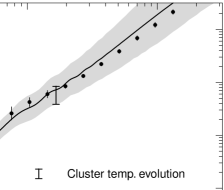
Figure 6.: Fluctuation power spectra where $\Delta^{2}(k)=V/(2\pi^{2})k^{3}P(k)$, but $\sigma_{8}\simeq\Delta(0.172hMpc^{-1})$. The shaded region gives the one $\sigma$ error on the present mass fluctuation power spectrum predicted by evolving the measured microwave background fluctuation spectrum to the present, under the assumption that $H_{0}=70$ km s^-1 Mpc^-1 $\pm 10\%$. The dots with errors are the galaxy fluctuation spectrum, while the single error bar is the value of $\sigma_{8}$ from an analysis of cluster temperature evolution by Henry (2000). The good agreement between the predicted spectrum and its observed normalization implies that clusters form from hierarchical growth. Original figure from Peacock et al. (2001)

The local abundance of clusters yields the following constraint: $\sigma_{8}\Omega_{m0}^{0.5}\simeq 0.5$. Figure 5 shows a recent example. Measuring the abundance at two epochs, that is measuring evolution, breaks this degeneracy and is a prime reason for making such measurements.

As an example, we give the results of our recent work (Henry 2000), which is fairly typical. None of the local samples described in Section 1.3 have complete temperature information, so we used a sample of 25 clusters originally from Piccinotti et al. (1982) with corrections for source confusion. Sixteen of these objects had temperatures from ASCA when we did the analysis. The only high redshift sample that has complete temperature information is the EMSS. We used 14 EMSS clusters selected by flux, all with ASCA temperatures and ROSAT HRI images. The average redshift of the local sample is 0.05 while that of the distant sample is 0.38. We found that $\Omega_{m0}=0.49\pm 0.12(1\sigma)\pm 0.23(2\sigma)$ and $\Omega_{m0}=0.44\pm 0.12(1\sigma)\pm 0.23(2\sigma)$ for open and flat cosmologies respectively. $\Omega_{m0}=1$ is excluded at $>>99\%$ confidence. For $\sigma_{8}$ we find $0.72\pm 0.10$ and $0.77\pm 0.15(1\sigma)$ for open and flat models respectively.

We show in Figures 5 and 6 a comparison of these results with some recent work not available when Henry (2000) was completed. Figure 5 compares the results deduced form weak gravitational lensing by field galaxies (Maoli et al., 2001) with those obtained from the local abundance of clusters (Pierpaoli et al., 2001). There is very good agreement with a similar degeneracy. Our results break the degeneracy as described above, again with very good agreement. Figure 6 shows the present power spectrum of density fluctuations (Peacock et al., 2001). The mass power spectrum is that predicted from cosmic microwave background, i.e. evolved from a redshift of $\sim 1000$ to the present, plus the assumption that $H_{0}=70$ km s^-1 Mpc^-1 $\pm 10\%$. The galaxy spectrum shows that galaxies exhibit a small bias with respect to the mass. The agreement between the cluster temperature normalization and the predicted mass spectrum shows that the tiny fluctuations present in the universe at $z\sim 1000$ really have grown by gravity to produce the clusters we observe today.

Figure 7.: Integral cluster temperature function. The open (filled) circles are the low (high) redshift cluster observations. The high redshift data come from the entire EMSS z $>0.3$ sample plus RX J0152.7-1357.

3.2. Improved Mass Function with Arbitrary $\Omega_{m0}$ and $\Omega_{\Lambda 0}$

Although the PS mass function is a good approximation to that obtained from large N-body simulations, it does predict too many low-mass clusters and too few high mass ones (see Jenkins et al., 2001). The ST mass function does a better job although it is not quite as good as the Jenkins et al. empirical fit. The ST mass function allows clusters to form via an ellipsoidal rather than the spherical PS collapse. We prefer the ST function because the empirical fits will presumably change with different numerical simulations; ST has the virtue that it stays the same. Another advance is the function $\Delta$ in the mass - temperature relation has finally been determined for arbitrary $\Omega_{m0}$ and $\Omega_{\Lambda 0}$ (Pierpaoli et al., 2001).

We have made a new determination of cluster temperature evolution. The local sample remains the same 25 clusters used in Henry (2000). All their temperatures are measured with ASCA by White (2000), thereby eliminating a possible systematic effect since all temperatures (but one in the high redshift sample) are measured with the same experiment. The high redshift sample is now all EMSS clusters with z $>0.3$ plus RX J0152.7-1357 with a temperature from Della Ceca et al. (2000). There are 20 clusters in the distant sample, the average redshift of which has increased to 0.45. We show the temperature functions in Figure 7. The temperatures exhibit the same moderate evolution as the luminosities discussed in Section 2.

Figure 8.: Constraints on the dark energy and dark matter content of the universe provided by the data in Figure 7. The solid lines are the one and two $\sigma$ contours using the ST mass function, while the dashed line is the one $\sigma$ contour from the PS mass function. The difference is small, $\sim 0.5\sigma$.

The recent theoretical advances permit us to constrain the geometry of the universe. We show these constraints in Figures 8 and 9. Figure 8 shows that the difference between the PS and ST mass functions is minor for the present sample size, $\sim 0.5\sigma$. Figure 9 compares the constraints provided by supernovae, the cosmic microwave background and cluster evolution. All three methods are concordant and nicely complementary, thereby diminishing the possibility that any one of them has significant systematic errors. It is clear that $\Omega_{m0}\sim 0.35$ and $\Omega_{\Lambda 0}\sim 0.65$ agrees with all determinations. It appears that the universe has significant amounts of dark matter and dark energy at present.

Figure 9.: Comparison of the constraints provided by cluster temperature evolution, supernovae and the microwave background. All three provide complementary constraints that show that the universe is presently dominated by dark energy. Original figure from Jaffe et al. (2001).

3.3. Summary of Cluster Temperature Evolution Constraints of Cosmological Parameters

Although the agreement exhibited by Figures 5, 6, and 9 is encouraging, there is a rather wider range in the best fit value of $\Omega_{m0}$ found by different investigators than would be expected from the quoted errors. One uncertainity is that clusters are selected by their flux, not temperature. The selection is quantified by specifying the surveyed solid angle as a function of flux. The flux can be straightforwardly converted to luminosity and redshift. The luminosity may be converted to temperature from the empirical cluster luminosity - temperature relation yielding the solid angle as a function of temperature and redshift. This second step is not as straightforward as the first. Although there is a relation, it has large scatter. At least the relation does not seem to evolve very much. The community has not yet settled on a preferred analysis method that incorporates this uncertainity. There is good agreement on the value of $\sigma_{8}$ among the various investigators or at least most results fall along the same $\sigma_{8}$ - $\Omega_{m0}$ degeneracy curve.

4. State of Very High Redshift Clusters

There are now about a dozen X-ray emitting clusters presently known at z $>0.75$. Chandra images are in hand for 8 of them (e.g. Cagnoni et al., 2001; Fabian et al., 2001; Jeltema et al., 2001; Stanford et al., 2001). All but 2 of these 8 are obviously not relaxed. This situation contrasts with that at low redshift where most clusters appear to be much closer to equilibrium (see the compilation of images in Mohr, Mathiesen, & Evrard, 1999). Although qualitative, this striking difference leads us to suspect that z $\sim 1$ is more likely the epoch of cluster formation than is the present.

Acknowledgments.

Thanks are due to the organizers of our conference for a great meeting in the magnificant setting of the Taroko National Park. I also want to thank my many collaborators with whom I have worked on cluster surveys over the years. These include: I. Gioia, C. Mullis, W. Voges, U. Briel, H. Böhringer and J. Huchra for the NEP; A. Vikhlinin, C. Mullis, I. Gioia, B. McNamara, A. Hornstrup, H. Quintana, K. Whitman, W. Forman, and C. Jones for the 160 deg²; H. Ebeling and A. Edge for the MACS. Most of the work described here will eventually appear as publications coauthored with them. H. Böhringer and H. Ebeling provided the digital data from Figures 20 and 10 of Böhringer et al. (2001a) and Ebeling et al. (2001) respectively.

References

Abell, G. O. 1958, ApJS, 3, 211

Bahcall, N. A. & Fan, X. 1998, ApJ, 504, 1

Blanchard, A., Sadat, R., Bartlett, J. G. & Le Dour, M. 2000, A&A, 362, 809

Böhringer, Schuecker, P., Guzzo, L., Collins, C. A., Voges, W., Schindler, S., Neumann, D. M., Cruddace, R. G., De Grandi, S., Chincarini, G., Edge, A. C., MacGillivray, H. T. & Shaver, P. 2001a, A&A, 369, 826

Böhringer, H., Collins, C. A., Guzzo, L., Schuecker, P., Voges, W., Neumann, D. M., Schindler, S., Chincarini, G., DeGrandi, S., Cruddace, R. G., Edge, A. C., Reiprich, T. H., & Shaver, P. 2001b, ApJ, submitted (astro-ph/0106243)

Borgani, S., Rosati, P., Tozzi, P., Stanford, S. A., Eisenhardt, P. E., Lidman, C., Holden, B., Della Ceca, R., Norman, C. & Squires, G. 2001, ApJ, in press (astro-ph/0106428)

Cagnoni, I., Elvis, M., Kim, D.-W., Mazzotta, P., Huang, J.-S., & Celotti, A. 2001, ApJ, in press (astro-ph/0106066)

DeGrandi, S., Böhringer, H., Guzzo, L., Molendi, S., Chincarini, G., Collins, C., Cruddace, R., Neumann, D., Schindler, S., Schuecker, P., & Voges, W. 1999, ApJ, 514, 148

Della Ceca, R., Scaramella, R., Gioia, I. M., Rosati, P., Fiore, F., & Squires, G. 2000, A&A, 353, 498

Donahue, M. & Voit, G. M. 1999, ApJ, 523, L137

Ebeling, H., Edge, A. C., Böhringer, H., Allen, S. W., Crawford, C. S., Fabian, A. C., Voges, W. & Huchra, J. P. 1998, MNRAS, 301, 881

Ebeling, H., Edge, A. C., Allen, S. W., Crawford, C. S., Fabian, A. C. & Huchra, J. P. 2000, MNRAS, 318, 333

Ebeling, H., Edge, A. C., & Henry, J. P. 2001, ApJ, 553, 668

Fabian, A. C., Crawford, C. S., Ettori, S., & Sanders, J. S. 2001, MNRAS, 332, L11

Gioia, I. M., Henry, J. P., Maccacaro, T., Morris, S. L., Stocke, J. T., & Wolter, A. 1990, ApJ, 356, L35

Gioia, I. M. & Luppino, G. A. 1994, ApJS, 94, 583

Henry, J. P., Branduardi, G., Briel, U., Fabricant, D., Feigelson, E., Murray, S., Soltan, A., & Tananbaum, H. 1979, ApJ, 234, L15

Henry, J. P., Gioia, I. M., Maccacaro, T., Morris, S. L., Stocke, J. T., & Wolter, A. 1992, ApJ, 389, 491

Henry, J. P. 2000, ApJ, 534, 565

Henry, J. P., Gioia, I. M., Mullis, C. R., Voges, W., Briel, U. G., Böhringer, H., & Huchra, J. P. 2001, ApJ, 553, L109

Jaffe, A. H. et al. 2001 Phys.Rev.Lett, 86, 3475

Jeltema, T. E., Canizares C. R., Bautz, M. W., Malm, M. R., Donahue, M. & Garmire, G. P. 2001, ApJ, in press (astro-ph/0107314)

Jenkins, A., Frenk, C. S., White, S. D. M., Colberg, J. M., Cole, S., Evrard, A. E. & Yoshida, N, 2001, MNRAS, 321 372

Jones, L., Ebeling, H., Scharf, C., Perlman, E., Horner, D., Fairley, B., Wegner, G. & Malkan, M. 2000, in “Large-Scale Structure in the X-ray Universe”, eds. M. Plionis & I. Georgantopoulos, Atlantisciences, Paris, France, p35

Maoli, R., Van Waerbeke, L., Mellier, Y., Schneider, P., Jain, B., Bernardeu, F., Erben, T. & Fort, B. 2001, A&A, 368, 766

Mohr, J. J. & Evrard, A. E. 1997, ApJ, 491, 13

Mohr, J. J., Mathiesen, B. & Evrard, A. E. 1999, ApJ, 517, 627

Mohr, J. J., Reese, E. D., Ellingson, E., Lewis, A. D. & Evrard, A. E. 2000, ApJ, 544, 109

Moretti, A., Guzzo, L., Campana, S., Covino, S., Lazzati, D., Longhetti, M., Molinari, E., Panzera, M. R. & Tagliaferri, G. 2001, astro-ph/0103348

Mullis, C. R., Vikhlinin, A., Henry, J. P., McNamara, B., Quintana, H., Gioia, I. M., Hornstrup, A., Forman, W. & Jones, C. 2002, in preparation

Nichol, R. C., Romer, A. K., Holden, B. P., Ulmer, M. P., Pildis, R. A., Adami, C., Merrelli, A. J., Burke, D. J. & Collins, C. A. 1999, ApJ, 521, L21

Peacock, J. A. 1999, Cosmological Physics, Cambridge: Cambridge University Press

Peacock, J. A., et al. 2001, Nature, 410, 169

Piccinotti, G., Mushotzky, R. F., Boldt, E. A., Holt, S. S., Marshall, F. E., Serlemitsos, P. J. & Shafer, R. A. 1982, ApJ, 253, 485

Pierpaoli, E., Scott, D., & White, M. 2001, MNRAS, 325, 77

Press, W. H. & Schechter, P. 1974, ApJ, 187, 425

Romer, A. K., Nichol, R. C., Holden, B. P., Ulmer, M. P., Pildis, R. A., Merrelli, A. J., Adami, C., Burke, D. J., Collins, C. A., Metevier, A. J., Kron, R. G. & Commons K. 2000, ApJS, 126, 209

Rosati, P., Borgani, S., Della Ceca, R., Stanford, A., Eisenhardt, P. & Lidman, C. 2000, in “Large-Scale Structure in the X-ray Universe”, eds. M. Plionis & I. Georgantopoulos, Atlantisciences, Paris, France, p13

Sheth, R. K. & Torman, G. 1999, MNRAS, 308, 119

Stanford, S. A., Holden, B., Rosati, P., Tozzi, P., Borgani, S., Eisenhardt, P. R. & Spinrad, H. 2001, ApJ, 552, 504, 2001

Viana, P. T. P. & Liddle, A. R. 1999, MNRAS, 303, 535

Vikhlinin, A., McNamara, B. R., Forman, W., Jones, C., Quintana, H. & Hornstrup, A. 1998, ApJ, 502, 558

White, D. A. 2000, MNRAS, 312, 663

Zwicky, F. & Herzog, F. 1983, “Catalog of Galaxies and Clusters of Galaxies”, Pasadena: California Institute of Technology