Variability of Active Galactic Nuclei

Abstract

Continuum and emission-line variability of active galactic nuclei provides a powerful probe of microarcsecond scale structures in the central regions of these sources. In this contribution, we review basic concepts and methodologies used in analyzing AGN variability. We develop from first principles the basics of reverberation mapping, and pay special attention to emission-line transfer functions. We discuss application of cross-correlation analysis to AGN light curves. Finally, we provide a short review of recent important results in the field.

1 Introduction

The study of multiwavelength variability of active galactic nuclei (AGNs) is now a major branch of the field, enabled largely by the availability of suitable facilities for long-term studies of faint sources at many wavelengths; some of the scientific arguments for development of these facilities have been based on exactly these programs, which are now leading to improved understanding of the AGN phenomenon. It is only within the last few years that the evidence for supermassive black holes in both active and non-active galaxies has gone from circumstantial to compelling, and the potentially most powerful technique for measuring black-hole masses in AGNs is through study of broad emission-line variability. The existence of accretion disks in AGNs is still far from proven, but the evidence for them is improving, again as a result of variability studies. Multiwavelength monitoring observations are beginning to show the relationships between variability in different bands, and the hope is that once the phenomenology is better known, our understanding of the physics will follow.

In this contribution, we will cover the basic characteristics of AGN variability and provide what we hope is some relevant historical background. Because of the current importance of emission-line variability studies, we will develop the theory of reverberation mapping from first principles. One of the most powerful and widely used tools in the analysis of emission-line and continuum variability data is the technique of cross-correlation, and we will therefore describe in some detail the application of this method to AGN data. Throughout this contribution, we will concentrate almost exclusively on non-blazar AGNs, those for which we believe most of the observed UV/optical emission originates in an accretion disk rather than in a relativistic jet: many of the techniques described here are also applicable to blazars, however. For a fairly recent discussion of blazar variability results, we refer the reader to the fine review by Ulrich et al.[86]. We emphasize that we intend for this contribution to be primarily instructional; this should not be misconstrued as a comprehensive review of the state of the field. Our intent is to provide both students and researchers who already have some familiarity with AGNs with enough background to read critically the current literature on AGN variability and understand the strengths and weaknesses of the method.

2 Background and Basic Phenomenology

AGNs show flux variations over the entire electromagnetic spectrum. Indeed, variability was one of the first recognized properties of quasars[51]^,[82]. Early investigations established that significant variations ($\raisebox{-2.15277pt}{$\;\stackrel{{\scriptstyle>}}{{\sim}}\;$}0.1$ mag) in the optical brightness of quasars could occur on time scales as short as days.

Detection of rapid variability in quasars was a remarkable discovery at the time because it implies that the size of the continuum-emitting region must be of order light days ($1\ \mbox{\rm lt-day}=2.6\times 10^{15}$ cm), based on source coherence arguments: for a source to vary coherently, the entire emitting region must be causally connected, which implies a maximum size for the source based on light-travel time. Suppose, for example, that the brightness of the source doubles in a week; we can immediately conclude that the emitting region must be no larger than one light week in radius on the basis of causality. We might suppose that in fact there are multiple emitting regions varying at random, but the number of such regions must be limited or the stochastic variations would be averaged out. Individually, then, the purported independent regions face a similar size limit from causality, and the conclusion that the emitting regions are very small cannot be avoided. Historically, this is the quasar problem: how can so much energy, the equivalent of as much as trillions of stars, be produced in a region that is about the size of the Solar System?

The detection of quasar variability was a critical part of the argument that AGNs are powered by supermassive black holes. The original arguments for supermassive black holes in AGNs were based on mass constraints from the Eddington limit and size constraints from variability[63]. The Eddington limit is the requirement that gravitational forces on an ionized gas exceed outward radiation pressure, which translates to a requirement that

$$M\geq M_{\rm Edd}\equiv 8\times 10^{5}\left(\frac{L}{10^{44}\ {\rm{\rm ergs\ s}^{-1}}}\right)\ {\rm M}_{\odot}\mbox{\ \ .}$$ (1)

Rapid variations, in some cases on time scales as short as a day, require an emitting region less than a light day in radius, which for a $10^{44}$ ergs s^-1 AGN corresponds to $\sim 10^{4}R_{\rm grav}$, where $R_{\rm grav}=GM/c^{2}$ is the gravitational radius. Later arguments for supermassive black holes in AGNs focussed on how to power AGNs by gravitational accretion[81]. The deep gravitational potential leads to an accretion disk that radiates most strongly across the UV/optical spectrum, and for AGN masses above the Eddington limit, the thermal emission should peak in the near UV. Indeed, then, the broad UV/optical feature known as the “big blue bump” can plausibly be identified with accretion-disk emission. Furthermore, the intense magnetic fields expected in disks could provide a mechanism for jet collimation.

2.1 Basic Characteristics of Variability

AGNs have been found to be variable at all wavelengths at which they have been observed. The variations appear to be aperiodic and have variable amplitude. While variability in high-luminosity AGNs (quasars) was reported soon after their discovery, variability in lower-luminosity AGNs (Seyfert galaxies) was not reported[25] until 1967, and was less dramatic. The reason for this is probably quite simple: most of the quasars that were monitored are now known to be the jet-dominated sources known as “blazars”. i.e., BL Lac objects and optically violent variables (OVVs). The optical identifications of quasars were based on coincidence with radio-source positions, which naturally led to biases towards radio-loud quasars, blazars in particular. Indeed, the original arguments about size and variability time scales in retrospect apply to the jets, not necessarily what we now identify as thermally emitting accretion disks. Nevertheless, the original conclusions about AGN sizes proved to be generally correct for both blazars and non-blazars.

UV/Optical Variability. Fig. 1 shows a light curve for a typical Seyfert 1 galaxy, NGC 5548, which will serve as a continuing example through this chapter as it is one of the best-studied objects of this class. While no periodic behavior has been identified, there are some basic parameterizations that allow us to characterize the variability. An example is shown in Fig. 2. We compare each flux measurement at an arbitrary time $t_{i}$ with the flux at every later time $t_{j}$. The quantity we show is the flux ratio as a function of the time interval between observations $\Delta t=t_{j}-t_{i}$, i.e., $\Delta\log F=\log F(t_{j})/F(t_{i})$, where in each case the contaminating flux due to starlight in the host galaxy (as shown in Fig. 1) has been first removed. Fig. 2 shows that NGC 5548 shows little variability on time scales shorter than a few days, but on time scales of several weeks or months, very large variations can be observed. We note in passing that the quantity shown here is closely related to the “structure function”. The structure function is simply the mean absolute value of $2.5\Delta\log F(\Delta t)$, i.e., the mean difference in magnitudes between observations separated by times $\Delta t$.

Figure 1: Optical (5100 Å) light curve of NGC 5548 from late 1988 to late 1996. The horizontal line indicates the constant contribution from starlight through the standard aperture used, which projects to $5^{\prime\prime}\times 7^{\prime\prime}\!.5$. From Peterson et al.⁷¹ ©1999 AAS.

Figure 2: Difference in optical flux as a function of interval between observations $\Delta t$ for the light curve shown in Fig. 1. The starlight contribution as shown in Fig. 1 has been subtracted off.

A common parameter to characterize variability is the mean fractional variation,

$$F_{\rm var}=\frac{\sqrt{\sigma^{2}-\delta^{2}}}{\left<f\right>}\mbox{\ \ ,}$$ (2)

where the quantities are (a) the mean flux for all $N$ observations,

$$\left<f\right>=\sum_{i=1}^{N}f_{i}\mbox{\ \ ,}$$ (3)

(b) the variance of the flux (as observed),

$$\sigma^{2}=\frac{1}{N}\sum_{i=1}^{N}\left(f_{i}-\left<f\right>\right)^{2}\mbox{\ \ ,}$$ (4)

and (c) the mean square uncertainty of the fluxes

$$\delta^{2}=\frac{1}{N}\sum_{i=1}^{N}\delta_{i}^{2}\mbox{\ \ .}$$ (5)

Even if the continuum is constant, there will still be apparent flux variations simply due to measurement uncertainties (noise); the virtue of $F_{\rm var}$ is that it adjusts the fractional variation downwards to account for the effect of random errors. The parameter $F_{\rm var}$ is thus sometimes referred to as the “excess variance.” In Fig. 3, we show $F_{\rm var}$ as a function of time interval UV and optical variations in NGC 5548. This shows that UV continuum variations are typically around 10–20% on time scales of about a month. The fractional variations in the optical are less pronounced, at least in part because of contamination of the fluxes by a large constant contribution from starlight in the host galaxy.

Figure 3: Variability parameter $F_{\rm var}$ from ultraviolet and optical continuum measurements of NGC 5548, as a function of interval between observations; the optical data used are those shown in Fig. 1. Courtesy of S. Collier.

X-Ray Variability. Rapid X-ray variability is a hallmark of AGNs (for a review, see Mushotzky et al.[54]). It is of historical importance since it effectively eliminates alternatives to supermassive black holes, e.g., massive stars or starbursts, as competing explanations for the high luminosities of AGNs. X-rays are expected to arise near the event horizon of the black hole, so the shortest time-scale X-ray variability is expected on a few times the crossing time

$$t_{\rm crossing}=\frac{R_{\rm grav}}{c}=10\left(\frac{M}{10^{6}\ {\rm M}_{\odot}}\right)\ {\rm s.}$$ (6)

Prior to the 1990s and the advent of RXTE, the best X-ray monitoring data was from EXOSAT, which was in a high-Earth orbit that allowed up to 80 hours of uninterrupted observations. The EXOSAT “long-looks” at variable AGNs established that variability is most rapid in low-luminosity systems.

A useful way to characterize variability is in terms of the “power density spectrum” (PDS), which is the product of the Fourier transform of the light curve and its complex conjugate. The PDS for AGNs is often parameterized as a power law,

$$P(f)=f^{-\alpha}\mbox{\ \ .}$$ (7)

The EXOSAT data[52] showed that AGN X-ray variations can be characterized by PDS indices in the range $1\raisebox{-2.15277pt}{$\;\stackrel{{\scriptstyle<}}{{\sim}}\;$}\alpha\raisebox{-2.15277pt}{$\;\stackrel{{\scriptstyle<}}{{\sim}}\;$}2$ over time scales of hours to months. The total power in the variations is given by integrating the PDS over all frequencies. Thus, the PDS must turn over at low frequencies (i.e., $\alpha$ as defined above must become less than unity) to prevent divergence in the total power. Such breaks in the PDS are observed in stellar-mass X-ray sources, and the turnover frequency correlates inversely with mass, though the fundamental reason for this is not understood. The basic idea is that the mass of the black hole can be inferred, since $M_{\rm BH}\propto R_{\rm grav}\propto t_{\rm crossing}$. If we scale AGNs relative to stellar-mass systems (which have turnover frequencies $f\approx 0.1$ Hz), we expect that the turnover frequencies for AGNs will occur at about $10^{-8}$ Hz. In only one case, NGC 3516, has there been a plausible detection of the turnover frequency. Edelson & Nandra[21] find that for this Seyfert 1 galaxy the turnover frequency is $f\approx 4\times 10^{-7}$ Hz, which corresponds to a time scale of about one month. The mass inferred, again scaling relative to stellar-mass systems, is in the range $10^{6}$–$10^{7}\,{\rm M}_{\odot}$.

Periodicities in X-ray light curves, which might reflect orbital or precession periods, have been searched for, but never found. As a historical footnote, however, it is worth mentioning that one such detection was claimed[53], namely a 12,000 s period in NGC 6814. However, ROSAT observations revealed that the variable source is in fact a foreground Galactic binary in the same field as the AGN[47].

2.2 Origin of the Variations

At a fundamental level, the physical origin of variations is not known, although accretion-disk instabilities are probably involved. For example, Kawaguchi et al.[37] show that continuum variations with a PDS of the form of Eq. (7) can be explained by magnetohydrodynamic instabilities, specifically disconnection events, within the disk. Variable accretion rates have also been considered. In some specific atypical cases, variations have been attributed to variable obscuration of the nuclear source and to microlensing due to stars in the host galaxy.

There are a number of important physical time scales that might be associated with variability. We include them here in the convenient form given by Edelson & Nandra[21]. The first of these is the crossing time already mentioned in Eq. (6), which we rewrite here as

$$t_{\rm crossing}=0.011M_{7}\left(\frac{r}{10R_{\rm grav}}\right)\ {\rm days},$$ (8)

which is the time it takes a radiative signal to cross the X-ray emitting region (assumed to be at $r\raisebox{-2.15277pt}{$\;\stackrel{{\scriptstyle<}}{{\sim}}\;$}10R_{\rm grav}$). Here $M_{7}$ is the black-hole mass in units of $10^{7}$ ${\rm M}_{\odot}$. Variations might also be expected on the time scale of the orbital period,

$$t_{\rm orbital}=0.33M_{7}\left(\frac{r}{10R_{\rm grav}}\right)^{3/2}\ {\rm days}.$$ (9)

Thermal instabilities might also cause variations on the time scale for their development,

$$t_{\rm thermal}=5.3\left(\frac{\alpha}{0.01}\right)^{-1}M_{7}\left(\frac{r}{10R_{\rm grav}}\right)^{3/2}\ {\rm days},$$ (10)

where $\alpha$ is the viscosity parameter. Mechanical instabilities may propagate as acoustic waves, which will travel at the sound speed and thus cross the disk on a time scale

$$t_{\rm sound}=33\left(\frac{r}{100H}\right)M_{7}\left(\frac{r}{10R_{\rm grav}}\right)^{3/2}\ {\rm days},$$ (11)

where $H$ is the disk thickness. And finally, the time scale over which the effects of variations in the accretion rate will propagate through the disk is given by the drift speed,

$$t_{\rm drift}=53000\left(\frac{r}{100H}\right)^{2}\left(\frac{\alpha}{0.01}\right)^{-1}M_{7}\left(\frac{r}{10R_{\rm grav}}\right)^{3/2}\ {\rm days}.$$ (12)

2.3 Blazar Variability

Variability properties of blazars are distinct from those of other non-beamed AGNs and should be mentioned separately. Blazars are characterized by extreme variability at all wavelengths. Unlike radio-quiet quasars or Seyfert galaxies, significant infrared and radio continuum variability is observed in blazars. Furthermore, the polarization of the continuum radiation is also significant (i.e., greater than a few percent), and the degree of polarization and amplitude of variability correlate with luminosity, which is the opposite case for non-blazars. Blazars are also the only sources detected at TeV energies, and the TeV fluxes can vary by as much as a factor of 10 in one day. All of these properties indicate that the continuum is dominated by emission from relativistic jets, as these characteristics suggest a non-thermal (synchrotron or inverse Compton) origin.

2.4 Emission-Line Variability

The broad emission lines in AGN spectra can vary both in flux and in profile. Over time scales of months and years, the changes can be very dramatic, but on shorter time scales they are more subtle. The first detection of emission-line variations was by Andrillat & Souffrin[2], based on photographic spectra of the Seyfert 1 galaxy NGC 3516. There were a few subsequent reports[83]^,[76], but these cases seemed to be widely regarded as “curiosities” that did not generate much follow-up work. The basic problem was that only very large changes could be detected photographically or with the intensified television-type scanners that were commonly used in AGN spectroscopy from the mid-1970s to mid-1980s. In the few cases where clear variations were detected, the changes were often dramatic; there were sometimes claims of Seyferts changing “type” as broad components of emission lines appeared or disappeared.

Pronounced variability of broad emission-line profiles was detected in the early 1980s by a number of investigators. Profile variations were originally thought to be due to excitation inhomogeneities; excitation pulses propagating through a broad-line region (BLR) with an ordered velocity field would produce features that could propagate across the profile with time. This concept led to the development of reverberation mapping, which is described in detail in Sec. 3. Peterson[61] reviews early work on emission-line variability.

A useful way to isolate the variable part of an emission line is shown in Fig. 4. The upper panel shows a mean spectrum formed from 34 individual HST spectra of NGC 5548. The lower panel shows the “root-mean square” (rms) spectrum which is formed from the same data simply by computing the rms flux at each wavelength. Constant features, such as narrow emission lines and host-galaxy flux, do not appear in the rms spectrum.

Figure 4: The top panel shows the mean spectrum computed from 34 HST spectra of the variable Seyfert 1 galaxy NGC 5548⁴⁰. The lower panel shows the rms spectrum based on variations around this mean. The rms spectrum thus isolates the variable components of the spectrum. Fluxes are in units of $10^{-15}$ ergs s^-1 cm^-2 Å^-1.

2.5 The First Monitoring Programs

The early 1980s saw the first attempts to monitor the UV/optical continuum and emission-line variations in Seyfert 1 galaxies. There were two reasons this happened when it did. First, there was a realization that variability afforded a powerful probe of the structure and kinematics of AGNs on projected scales of microarcseconds. Variability was recognized as an important new tool with which to study enigmatic quasars. Second, the right technology for such investigations became widely available: it was possible to attempt such programs on account of (a) IUE, which for the first time allowed precision UV spectroscopy of low-redshift extragalactic objects, and (b) the proliferation of linear electronic detectors (first Reticons and Image Dissector Scanners, and later CCDs) on moderate-size (1–2m) ground-based telescopes.

One of the first significant monitoring programs was a multiple-year IUE-based program on NGC 4151, which was carried out by a European consortium led by M.V. Penston and M.-H. Ulrich[84]. Ultraviolet spectra were obtained with a typical sampling interval of 2–3 months. The program showed that variations in the UV and optical continua were closely coupled. It also revealed that the emission-line flux variations are correlated with continuum variations, but that different lines respond in different ways, both in amplitude and in time scale. These data also showed a complicated relationship between UV and X-ray variations and led to the discovery of variable absorption lines in the ultraviolet.

The galaxy NGC 4151 was also monitored spectroscopically in the optical at Lick Observatory by Antonucci & Cohen[4]. They found that the Balmer lines seemed to respond to continuum variations on a time scale less than around one month (their typical sampling interval). They also found that relative to H$\beta$ and H$\alpha$, the higher-order Balmer lines and He ii $\lambda 4686$ varied with higher amplitudes.

Arakelian (Akn) 120 was the first higher-luminosity Seyfert that was monitored fairly extensively in the optical[64]^,[65] as a result of dramatic Balmer-line profile changes that had been detected earlier[26]^,[38]^,[80]. Peterson et al.[65] found that the time scale for the response of H$\beta$ to continuum variations suggested a BLR size of less than 1 light month across. This was a surprising result as it suggested that there was a serious problem with existing estimates of sizes of the BLR that were based on photoionization equilibrium modeling, as these indicated the BLR should be about an order-of-magnitude larger than this. The upper limit on the BLR size was similar to that obtained by Antonucci & Cohen[4] for NGC 4151, but because Akn 120 is a higher-luminosity source, the monthly sampled data provided a more critical challenge to BLR models.

Not surprisingly, the results from these earlier monitoring programs were controversial. Several observational problems could be identified:

1. Undersampling of the variations. The variations tended to be undersampled because the original programs for monitoring Seyfert galaxies were designed for BLRs that were thought to be many light months in size. For example, in the case of Akn 120, Peterson et al.[65] were looking for profile structures that were expected to cross the line profile on a time scale of a year or so, and monthly observations should have been sufficient to carry out this program. There was certainly at the time no reason to believe that higher sampling rates should be required; indeed, proposals to observe AGNs as often as once per month were sometimes deemed to be “oversampled” by telescope allocation committees! There is no obvious algorithm to determine whether or not the variations that have been observed are undersampled, but it is quite obvious that if the results depend on individual data points, the light curve is almost certainly undersampled and any conclusions drawn must be eyed with suspicion. A very simple operational criterion for adequate sampling is that if the results do not change much when individual points are removed from the light curve, the light curve is probably not seriously undersampled. A nice simple test is to divide a light curve into two parts, one comprised of the even-numbered points (i.e., second, fourth, etc., in the time-ordered series) and one comprised of the odd-numbered points. If the two light curves are still very similar, i.e., the important features appear in both light curves, then the original light curve is probably adequately sampled.

2. Low S/N of the light curves. If the detected variations are not large compared to the signal-to-noise ratio (S/N) of typical data, then spurious results can be obtained. Stated another way, $F_{\rm var}$ (Eq. (2)) must be significantly greater than zero. This was a serious issue in the case of some of the earlier data obtained with image dissector scanners and Reticon arrays, for which uncertainties in AGN line and continuum fluxes were typically around 8–10%. To a large degree, this problem has been obviated by use of CCDs, for which typical errors in the 1–3% range are routinely achieved.

3. Systematic errors. There are two sometimes-related types of insidious errors that can adversely affect time series analysis: (a) correlated continuum/line errors, and (b) aperture effects.

   Correlated errors are due to systematic flux-calibration errors. Basically, if the flux calibration of a spectrum is incorrect, both the continuum and emission-line fluxes measured from it will be in error in the same sense; if the calibration is too high, both the emission-line and continuum fluxes will be too high. This introduces an artificial correlation between the line and continuum at zero lag, and can thus bias the measurement of the true lag between them to artificially small values.

   Aperture effects occur when the amount of flux entering a spectrograph is not fixed, on account of pointing or guiding errors, or variations in seeing in the case of ground-based observations. In point-like sources like stars, this affects only the overall photometric accuracy. In nearby AGNs, however, both the narrow-line region (NLR) and host-galaxy are spatially resolved, and the aperture geometry, centering and guiding, and seeing variations can lead to apparent spectral variations. Depending on their nature, aperture effects can cause either correlated, uncorrelated, or even anticorrelated errors in the line and continuum fluxes.

2.6 Spectrophotometric Flux Calibration

In this section, we will outline some of the important considerations for flux calibration of spectroscopic monitoring data, directed primarily towards ground-based optical observers.

In AGNs, aperture effects arise because the source is comprised of multiple components, some of which have angular structure on scales similar to the width of the point-spread function (PSF). The basic requirement for accurately flux-calibrating AGN spectra is that stable fractions of light from the AGN continuum source and BLR (both point-like at even the 0$.\!\!^{\prime\prime}$01 level) and the NLR and the host galaxy (both extended even at arcsecond levels) must enter the aperture. We note that even in the case of space-based observations, there is a trade-off between aperture size and pointing uncertainty: the goal is to minimize the amount of host-galaxy starlight entering the aperture (arguing for a smaller aperture), while ensuring that the amount of admitted starlight is constant (arguing for an aperture large relative to the pointing accuracy of the telescope). In the UV, however, this is a less-significant problem because the host galaxy is so much fainter than the AGN itself.

Mitigation of aperture effects is one of the most important considerations for a ground-based monitoring program. This is important to keep in mind, as most AGN observers are used to background-limited observations of point sources, and this calls for adjusting the slit width for variations in seeing in order to optimize the S/N of the data. However, this is exactly the wrong thing to do if you are monitoring Seyfert galaxy variations, since calibration accuracy is almost always determined by systematics rather than photon statistics. Most observers do know that you need to open up the aperture for absolute spectrophotometry, however, and this is precisely what needs to be done in monitoring programs, as we will explain below.

The standard method of absolute flux calibration is to determine from observations of spectrophotometric standard stars how counts per second per pixel on the detector translates to flux per unit wavelength. However, standard absolute spectrophotometry is far too inaccurate for ground-based AGN monitoring; the typical accuracy that can be achieved on photometric nights is about 5%. Furthermore, at most observing sites, only a relatively small fraction of nights are of sufficient quality and stability for absolute spectrophotometry to be useful. Even at a good site like Kitt Peak, fewer than 1/3 of the nights are photometric. However, more than 2/3 of all nights (including bright time) are good enough to get quality spectra of bright AGNs with a 1–2-m telescope with a typical photometric accuracy about 15%. Since we need a high rate of sampling and do not wish to discard more than half of the potentially usable nights, secondary higher-accuracy calibration methods must be used. In ground-based AGN monitoring, there are two commonly used high-accuracy flux-calibration methods, which we outline below:

1. Relative spectrophotometry. This method involves simultaneous observation of a nearby field star (that must be shown to be non-variable!) in long-slit mode. Absolute calibration can be achieved by calibrating spectra of the comparison star in the usual fashion described above on nights of photometric quality. This method has been used to attain internal (relative) accuracies of $\sim 1$–2%[16]^,[36]. The limitations of this method are (a) an extremely accurate slit response function (i.e., relative sensitivity as a function of position in the slit) is required, (b) a large slit and high pointing and guiding accuracy is required to avoid aperture/seeing effects, and (c) this method is difficult to use shortward of $\sim 4000$ Å because the requirement of fixed position angle (to observe the AGN and comparison star simultaneously) leads to atmospheric dispersion problems.

2. Internal calibration. This is based on using a constant-flux component in the spectrum (e.g., narrow emission lines) to refine absolute calibration. In this way, internal accuracies of $\sim 2$% have been routinely achieved[69]^, [71]. The [O iii] $\lambda\lambda 4959$, 5007 doublet is excellent for this method because these lines are strong, relatively unblended, and close in wavelength to H$\beta$ and He ii $\lambda 4686$. Unlike the broad lines, the narrow lines are almost always expected to be constant in flux. The light-crossing time for the NLR is large (typically 100–1000 years) as is the recombination time (about 100 years; see Eq. (17) in Sec. 3), so any short-term variability is smeared out. This method also has limitations: (a) most narrow lines are blended and/or weak, (b) the method works best at reasonably high spectral resolution, when the narrow-lines are at least partially resolved, and (c) in nearby AGNs, the NLR is often extended on scales of arcseconds, which introduces the possibility of aperture effects.

The last of these problems deserves serious consideration. If the NLR is extended, measuring a consistent flux is difficult due to aperture effects, as described above; either centering and guiding errors or differences in the seeing between observations can alter the calibration of the spectrum. However, it is possible to understand the nature of these effects so that in principle one can correct for them, or at minimum one can pursue mitigation strategies to reduce their influence. To do this, one must know (a) the surface brightness distributions of the extended components (the host galaxy and the NLR) and (b) the PSF, including the seeing component, for the instrument at the time of the observations.

With a good model for the surface brightness distributions, we can still use the narrow-lines for flux calibration, and then apply a seeing-dependent flux correction[89]^,[68]. Even if the seeing is not measured, such models can be used to give us an idea of how badly our observations might be adversely affected by seeing variations. As an example, the corrections to the point-source fluxes (broad lines and AGN continuum) and host galaxy flux that need to be applied in the case of NGC 4151 are shown in Fig. 5 for different aperture geometries. We can readily conclude from these diagrams that seeing-dependence of the correction factors is smaller for larger apertures, as can be expected intuitively. A useful generalization is that the corrections for seeing effects are generally not necessary if the aperture in both dimensions is larger than the worst seeing, as measured by the full-width at half-maximum (FWHM) of a stellar image.

Figure 5: Aperture corrections (as defined by Peterson et al.⁶⁸) for NGC 4151. These are multiplicative adjustments that must be made to (a) the broad emission-line and AGN continuum fluxes (top panel) and (b) the host-galaxy starlight contribution (bottom panel) as a function of seeing when the spectra are calibrated by assuming a constant flux in [O iii] $\lambda\lambda 4959$, 5007. The reference point is a $5^{\prime\prime}\times 7\hbox{$.\!\!^{\prime\prime}$}5$ aperture and seeing ${\rm FWHM}=1\hbox{$.\!\!^{\prime\prime}$}3$. For sufficiently large apertures, the correction is negligible under even quite poor observing conditions; for small apertures, seeing effects can produce apparent variability. The starlight correction factor for the $10^{\prime\prime}\times 13^{\prime\prime}$ aperture has a value of $\sim 1.6$ and varies only weakly with seeing.

2.7 Requirements for a Successful Monitoring Program

In order to avoid misleading systematic errors of the sort discussed thus far, care must be taken in designing an observational monitoring program. The fairly obvious basic requirements that we should keep in mind are:

1. The monitoring program must have sufficient sampling. Specifically, the observations should be closely spaced in time relative to physical time scales of interest. In terms of total duration, the program should be at least three times as long as the longest time scale to be investigated.

2. The S/N of the light curve must be high enough to detect variations on the shortest interesting physical time scale. Inspection of Fig. 2, for example, demonstrates that if you can measure continuum fluxes to only 10% accuracy, 3$\sigma$ detections of continuum variability in Seyfert 1 galaxies will be extremely rare on time scales as long as months.

3. Systematic effects must be obviated. The data must be as homogeneous as possible. The easiest way to do this is to acquire the data with a single instrument in a stable configuration that is suitable for all the observing conditions expected over the duration of the program.

3 Theory of Reverberation Mapping

After emission-line variability was detected, it became clear to a number of investigators[5]^,[23]^,[7]^,[10]^,[3] that the kinematics and the geometry of the BLR can be tightly constrained by characterizing the emission-line response to continuum variations. The time delay between continuum and emission-line variations are ascribed to light travel-time effects within the BLR; the emission lines “echo” or “reverberate” to the continuum changes. The Blandford & McKee paper[7], regarded as the seminal paper in the field, first introduced the term “reverberation mapping” to describe this process. Reviews of progress in reverberation mapping are provided by Peterson[62] and Netzer & Peterson[58].

Because the emission lines vary with the UV/optical continuum (with some small time delay), we can immediately draw several important conclusions:

1. The line-emitting clouds are close to the continuum source, i.e., the light-travel time across the BLR is small.

2. The line-emitting clouds are optically thick. If they were optically thin, the line emission from them would change little as the continuum varied.

3. The observable UV/optical continuum variations are closely related to variations of the ionizing continuum ($\lambda<912$ Å, $h\nu\geq 13.6\,{\rm eV}$).

This information provides the crucial underpinning for the assumptions detailed below. But before we proceed any further, we need to remind ourselves of some of the basic characteristics of the line-emitting gas, much of which we derive by comparing the observed line spectra with the predictions of photoionization equilibrium computer codes (see the contribution by Netzer for a more complete discussion). In general, photoionization equilibrium models of the line-emitting clouds are parameterized by the shape of the ionizing continuum, elemental abundances, and an “ionization parameter”

$$U=\frac{Q({\rm H})}{4\pi r^{2}cn_{\rm e}}\mbox{\ \ ,}$$ (13)

where

$$Q({\rm H})=\int^{\infty}_{\nu_{1}}\frac{L_{\nu}}{h\nu}\ d\nu$$ (14)

is the number of hydrogen-ionizing ($h\nu_{1}=13.6$ eV) photons emitted per second by the central source.

Essentially, $U$ characterizes the ionization balance within the cloud, as $Q({\rm H})/r^{2}$ is proportional to the number of photoionizations occurring per second at the incident face of the cloud, and $n_{\rm e}$ is proportional to the recombination rate. For a typical Seyfert 1 galaxy (NGC 5548)

$$Q({\rm H})\approx 10^{54}\,h_{0}^{-2}\ {\rm photons\ s}^{-1}\mbox{\ \ ,}$$ (15)

where $h_{0}$ is the Hubble constant in units of 100 km s^-1 Mpc^-1. By taking the electron density to be $n_{\rm e}\approx 10^{11}$ cm^-3and the distance to the central source to be 10 light days, we find $U\approx 0.1$. The line-emitting clouds are ionized to the “Strömgren depth”,

$$R_{\rm S}=\frac{Uc}{\alpha_{\rm B}n_{\rm e}}\approx 10^{11}\ {\rm cm}\mbox{\ \ ,}$$ (16)

at which point virtually all of the incident ionizing photons have been absorbed. In BLR clouds, the region beyond the Strömgren zone is partially ionized, $n({\rm H}^{+})\approx 0.1n({\rm H}^{0})$, and heated primarily by far infrared radiation[24] and partly by high-energy X-rays[45]. In Eq. (16), $\alpha_{\rm B}$ is the Menzel–Baker case B recombination coefficient[59].

3.1 Reverberation Mapping Assumptions

There are a number of simplifying assumptions that we can now make:

1. The continuum originates in a single central source. The size of an accretion disk around a supermassive (say, $10^{7-8}$ ${\rm M}_{\odot}$) black hole is of the order of $10^{13-14}$ cm. A typical size for the BLR in the same system would be of order a few light days, i.e., $\sim 10^{16}$ cm. Note that it is specifically not required that the continuum source emits radiation isotropically, though this is a useful starting point. The “point-source” assumption greatly simplifies the reverberation process. However, we should mention that the point-source assumption is probably not applicable to X-ray reverberation, as the Fe K$\alpha$ emission and the hard X-rays that drive this line probably arise in regions that are of similar size, and perhaps co-spatial[79].

2. Light-travel time is the most important time scale. We assume specifically that emission-line clouds respond instantaneously to changes in the continuum flux. The time scale to re-establish photoionization equilibrium is the recombination time,

   $$\tau_{\rm rec}=\left(n_{\rm e}\alpha_{\rm B}\right)^{-1}\approx 40\left(\frac{n_{\rm e}}{10^{11}\,{{\rm cm}^{-3}}}\right)^{-1}{\rm s.}$$ (17)

   The time it takes a Lyman $\alpha$ photon to diffuse outward from the Strömgren depth is about 20 times the direct light-travel time[35],

   $$\tau_{\rm diff}=20\frac{R_{\rm S}}{c}\approx 20\frac{U}{n_{\rm e}\alpha_{\rm B}}\approx 60\left(\frac{n_{\rm e}}{10^{11}\,{{\rm cm}^{-3}}}\right)^{-1}\ {\rm s.}$$ (18)

   We also need to carry out our reverberation-mapping experiment on a time scale short enough that the structure of the BLR can be assumed to be stable. The dynamical, or cloud-crossing, time scale for the BLR is typically

   $$\tau_{\rm dyn}=\frac{r}{V_{\mbox{\tiny FWHM}}}\approx 3-5\ {\rm years},$$ (19)

   where $V_{\mbox{\tiny FWHM}}$ is the Doppler width of the broad line for which the response time $\tau=r/c$ has been measured. Any reverberation-mapping experiment has to be short relative to the crossing time or the structural information might be washed out by cloud motions.

3. There is a simple, though not necessarily linear, relationship between the observed continuum and the ionizing continuum.

3.2 The Transfer Equation

Under these assumptions, the relationship between the continuum and emission lines can be written in terms of the “transfer equation”,

$$L(V_{z},t)=\int^{\infty}_{-\infty}\Psi(V_{z},\tau)\,C(t-\tau)\,d\tau\mbox{\ \ .}$$ (20)

Here $C(t)$ is the continuum light curve, $L(V_{z},t)$ is the emission-line flux at line-of-sight velocity $V_{z}$ and time $t$, and $\Psi(V_{z},\tau)$ is the “transfer function” at $V_{z}$ and time delay $\tau$. Inspection of the transfer equation shows that the transfer function is simply the time-smeared emission-line response to a $\delta$-function outburst in the continuum. Note that causality requires that the lower limit on the integral is $\tau=0$.

Solution of the transfer equation to obtain the transfer function is a classical inversion problem in theoretical physics: the transfer function is essentially the Green’s function for the system. Unfortunately, it is difficult to find a stable solution to such equations, especially when the data are noisy and sparse, as they usually are in astronomical applications.

In practice, most analyses have concentrated on solving the velocity-independent (or 1-d) transfer equation,

$$L(t)=\int^{\infty}_{-\infty}\Psi(\tau)\,C(t-\tau)\,d\tau\mbox{\ \ ,}$$ (21)

where both $\Psi(\tau)$ and $L(t)$ represent integrals over the emission-line width.

The transfer equation is a linear equation. In reality, however, the relationship between the observed continuum and the emission-line response is likely to be nonlinear. We therefore approximate $C(t)=\bar{C}+\Delta C$ and $L(t)=\bar{L}+\Delta L$, where $\bar{C}$ and $\bar{L}$ represent constants, usually the mean value of the continuum and line flux, respectively. We can then treat deviations from the mean as linear perturbations and the equation we actually solve is

$$\Delta L(t)=\int^{\infty}_{-\infty}\Psi(\tau)\,\Delta C(t-\tau)\,d\tau\mbox{\ \ .}$$ (22)

Most existing data sets are inadequate for transfer-function solution, and simpler analyses are used. The most commonly used tool in analysis of AGN variability is cross-correlation, which will be discussed in detail in Sec. 4.

3.3 Isodelay Surfaces

Suppose for the moment that the BLR consists of clouds in a thin spherical shell of radius $r$. Further suppose that the continuum light curve is a simple $\delta$-function outburst. Continuum photons stream radially outward and after travel time $r/c$, about 10% of these photons (using a typical “covering factor”) are intercepted by BLR clouds and are reprocessed into emission-line photons. An observer at the central source will see the emission-line response from the entire BLR at a single instant with a time delay of $2r/c$ following the continuum outburst. At any other location, however, the summed light-travel time from central source to line-emitting cloud to observer will be different for each part of the BLR. In the case of a $\delta$-function outburst, at any given instant, the parts of the BLR that the observer will see responding are all those for which this total path length is identical; at any given time delay, the part of the BLR that the observer sees responding is the intersection of the BLR distribution and an “isodelay surface.” Astronomers, on account of their familiarity with conic sections, can readily recognize that the shape of the isodelay surface is an ellipsoid with the continuum source at one focus and the observer at the other; the light-travel time from central source to BLR cloud to observer is constant for all points on the ellipsoid. Since the observer is virtually infinitely distant from the source, the isodelay surface becomes a paraboloid, as shown schematically in Fig. 6. The figure shows the BLR as a ring intersected by several isodelay surfaces, labeled in terms of their time delay in units of $r/c$. Relative to the continuum, points along the line of sight to the observer are not time delayed (i.e., $\tau=0$). Points on the far side of the BLR are delayed by as much as $2r/c$, the time it takes continuum photons to reach the BLR plus the time it takes line photons emitted towards the observer to return to the central source on their way to the observer.

Figure 6: The circle represents a cross-section of a shell containing emission-line clouds. The continuum source is a point at the center of the shell. Following a continuum outburst, at any given time the observer far to the left sees the response of clouds along a surface of constant time delay, or isodelay surface. Here we show five isodelay surfaces, each one labeled with the time delay (in units of the shell radius $r$) we would observe relative to the continuum source. Points along the line of sight to the observer are seen to respond with zero time delay. The farthest point on the shell responds with a time delay $2r/c$.

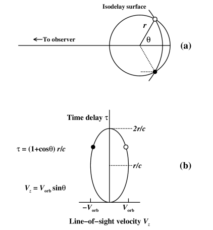
Figure 7: The upper diagram shows a ring (or cross-section of a thin shell) that contains line-emitting clouds, as in Fig. 6. An isodelay surface for an arbitrary time is given; the intersection of this surface and the ring shows the clouds that are observed to be responding at this particular time. The dotted line shows the additional light-travel time, relative to light from the continuum source, that signals reprocessed by the cloud into emission-line photons will incur (Eq. (23)). In the lower diagram, we project the ring of clouds onto the line-of-sight velocity/time-delay ($V_{z},\tau$) plane, assuming that the emission-line clouds in the upper diagram are orbiting in a clockwise direction (so that the cloud represented by a filled circle is blueshifted and the cloud represented by an open circle is redshifted).

Essentially, the transfer function measures the amount of line emission emitted at a given Doppler shift in the direction of the observer as a function of time delay $\tau$. The value of the transfer function at time delay $\tau$ is computed by summing the emission in the direction of the observer at the intersection of the BLR and the appropriate isodelay surface. For a thin spherical shell, the intersection of the BLR and an isodelay surface is a ring of radius $r\sin\theta$, where the polar angle $\theta$ is measured from the observer’s line of sight to the central source, as shown in Fig. 7. The time delay for a particular isodelay surface is the equation for an ellipse in polar coordinates,

$$\tau=(1+\cos\theta)r/c\mbox{\ \ ,}$$ (23)

as is obvious from inspection of Fig. 7. The surface area of the ring of radius $r\sin\theta$ and angular width $r\,d\theta$ is $2\pi(r\sin\theta)\,r\,d\theta$, and assuming that the line response per unit area on the spherical BLR has a constant value $\varepsilon_{0}$, the response of the ring can be written as

$$\Psi(\theta)=2\pi\varepsilon_{0}r^{2}\sin\theta\,d\theta\mbox{\ \ ,}$$ (24)

where $0\leq\theta\leq 2\pi$. From Eq. (23), we can write

$$d\tau=-(r/c)\sin\theta\,d\theta\mbox{\ \ ,}$$ (25)

so putting the response in terms of $\tau$ rather than $\theta$, we obtain

$$\Psi(\tau)\,d\tau=\Psi(\theta)\left|\frac{d\theta}{d\tau}\right|\,d\tau=2\pi\varepsilon rc\ d\tau$$ (26)

for values from $\tau=0$ ($\theta=2\pi$) to $\tau=2r/c$ ($\theta=0$). The transfer function for a thin spherical shell is thus constant over the range $0\leq\tau\leq 2r/c$.

3.4 Transfer Functions for a Variety of Simple Models

The simple analytic calculation in the last section was intended to be illustrative and serve as a reference point. We will now expand on this with more general geometries, and also incorporate information from Doppler motion along the line of sight. We will derive some transfer functions for other simple models, focusing on three: (a) systems of clouds in circular Keplerian orbits, illuminated by an isotropic continuum, (b) biconical outflows, and (c) disks of random inclination. All these are physically plausible, and can produce “double-peaked” emission-line profiles, which are sometimes seen in AGNs, though not all of these models necessarily do this. We will start with the simplest models and progress to more complicated models. Much of this discussion is drawn from discussions of transfer functions in the literature[93]^,[60]^,[24]^,[30]^,[31].

Suppose line-emitting clouds are on a circular orbit at inclination $i=90$^o; imagine that the circle in Fig. 7a represents this orbit seen face on. The line response from the clouds at the intersection of an arbitrary isodelay surface and the circular orbit will be at time delay $\tau=(1+\cos\theta)r/c$ and line-of-sight velocities $V_{z}=\pm V_{\rm orb}\sin\theta$, where $V_{\rm orb}=(GM/r)^{1/2}$, the circular orbital speed. It is easy to see that the circular orbit projects to an ellipse in the line-of-sight velocity/time-delay ($V_{z},\tau$) plane with semiaxes $V_{\rm orb}$ and $r/c$, as shown in Fig. 7b. This simple example is important because it is straightforward to generalize it to both disks (rings of different radii) and shells (rings at different inclinations).

Figure 8: Here we take the circular ring shown in Fig. 7 and show how its projection on $V_{z},\tau$ changes as the inclination is decreased from 90^o; in the time-delay direction, the axis contracts to $2r\sin i/c$, and in the velocity direction it decreases to $2V_{\rm orb}\sin i$.

Figure 9: Transfer function for a thin spherical shell. The upper left panel shows in grey scale the two-dimensional transfer function, i.e., the observed emission-line response as a function of line-of-sight velocity $V_{z}$ and time delay $\tau$. The upper right panel shows the one-dimensional transfer function, i.e., the two-dimensional transfer function integrated over $V_{z}$, which is the response of the total emission line as a function of time (cf. Eq. (26)). The lower left panel shows the emission-line response integrated over time delay; this is the profile of the variable part of the line. The specific model here is comprised of emission-line clouds in circular orbits of radius $r=10$ light days and random inclinations ($0^{\rm o}\leq i\leq 180^{\rm o}$), orbiting around a central black hole of mass $10^{8}$ ${\rm M}_{\odot}$. In this model, the line emission from each cloud is isotropic ($A=0$).

First we consider the generalization to a shell. We can construct a shell from a distribution of circular orbits, with inclinations ranging from $i=0^{\rm o}$ to $i=180$^o. As we decrease the inclination of the circular orbit in Fig. 7a from $i=90^{\rm o}$, we see that the range of time delays will decrease from [0, $2r/c$] to [$(1-\sin i)r/c$, $(1+\sin i)r/c$], and similarly the line-of-sight velocity range will decrease from [$-V_{\rm orb}$, $+V_{\rm orb}$] to [$-V_{\rm orb}\sin i$, $+V_{\rm orb}\sin i$], as we show schematically in Fig. 8. At the limiting case $i=0^{\rm o}$, the time delays all contract to $r/c$, since the light travel-time paths for all points on a face-on ring are the same, and the velocities all contract to $V_{z}=0$, because the orbital velocities are now perpendicular to the line of sight. Thus, the transfer function looks like a series of ellipses as in Fig. 8b that with decreasing inclination contract down to a single point at $V_{z}=0$ and $\tau=r/c$ when $i=0^{\rm o}$. We can construct such a transfer function by using a Monte Carlo method that places BLR clouds randomly across the surface of the shell, and the result we get is shown in Fig. 9, which corresponds to a thin shell of radius 10 light days and a central mass of $10^{8}\,{\rm M}_{\odot}$. We have also integrated this transfer function over $\tau$ and $V_{z}$ to obtain the emission-line profile and the one-dimensional transfer function, respectively. In the particular case of a thin spherical shell, we see that both of these are simple rectangular functions, as we showed analytically for the one-dimensional transfer function (Eq. (26)).

The first complication that we might consider is anisotropic line emission by the BLR clouds. Physically, this will occur if the BLR clouds themselves are optically thick in the lines as well as the continuum. In this case, most of the line radiation emitted by the clouds will be from the side of the cloud facing the continuum source, i.e., the line emission is directed back towards the continuum source. A simple parameterization of asymmetric line emission is to describe the apparent emissivity of a cloud as

$$\varepsilon(\theta)=\varepsilon_{0}\left(1+A\cos\theta\right)\mbox{\ \ ,}$$ (27)

where $\varepsilon_{0}$ is constant and the parameter $A=0$ for isotropic emission and $A=1$ for completely anisotropic emission; the latter case is appropriate for spherical clouds with inward-facing surfaces that are uniformly bright. In principle, $A$ can be estimated by photoionization modeling, though in practice the values are highly uncertain on account of limitations in the accuracy of the radiative transfer codes (see the contribution by Netzer). It is certainly expected that $A\approx 1$ for Ly$\alpha$, at least, and models suggest approximate values $A\approx 0.7$ for C iv and $A\approx 0.8$ for H$\beta$[24]. The main effect of anisotropic emission is to increase the measured lag for a given geometry because the apparent response of the near side of the BLR is suppressed. For a thin shell of radius $r$, the mean time delay is $\tau=(1+A/3)r/c$. Fig. 10 shows the transfer function for the same thin spherical shell model of Fig. 9, but in this case with highly anisotropic ($A=1$) line response.

Figure 10: Transfer function for a thin spherical shell, as in Fig. 9, except with completely anisotropic ($A=1$) line emission, i.e., all of the emission line flux from each cloud is directed back towards the continuum source.

In addition to anisotropic line response, we can also consider anisotropic illumination of the BLR clouds by the continuum source. As an example, consider the case where BLR clouds are illuminated by biconical beams of semi-opening angle $\omega$; the limiting case as $\omega$ approaches zero would be a narrow jet-like pencil beam, and the case $\omega=90^{\rm o}$ corresponds to an isotropic continuum. We start by examining the response of an edge-on ($i=0^{\rm o}$) circular ring, as we show in Fig. 11, which is exactly like Fig. 7, but with only part of each orbit illuminated by the continuum source. We earlier generalized the result for a shell, going from Fig. 7 to Fig. 8 as we decreased the inclination of the ring; doing this again, we see in Fig. 12 how the two-dimensional transfer function is altered by anisotropic illumination. We note specifically the absence of any response near $\tau=0$ and $\tau=2r/c$ since the bicones shown do not illuminate BLR clouds directly along the observer’s axis. Similarly there is also no response around $\tau=r/c$ due to the absence of response of clouds at $\theta\approx 90^{\rm o}$.

Figure 11: A ring-like line-emitting region and its projection into the $V_{z},\tau$ plane is shown, as in Figs. 7 and 8, though in this case with a biconical continuum geometry. In the case shown here, the beam semi-opening angle is $\omega=30$^o, and the beam is inclined to the observer by $i=45$^o. Again assuming that clouds on the ring are orbiting in the clockwise direction, we highlight in the lower diagram the regions in the ($V_{z},\tau$) plane that will produce an emission-line response; there is no emission-line response from clouds not illuminated by the continuum beam.

So far we have restricted our attention to “thin” geometries, i.e., single orbits and shells. Generalization to “thick” geometries, e.g., disks and shells with different inner and outer radii, is trivial: the response of a disk can be computed by integrating over a series of circular orbits, and the response of a thick shell is obtained by integrating over a series of shells. In Fig. 13, we illustrate this concept by showing the response from two rings.

Figure 12: Transfer function for a thin spherical shell, as in Fig. 9, except with an anisotropic continuum source. In the example shown, the beam opening angle is $\omega=30$^o and the inclination is $i=45$^o, as in Fig. 11.

Figure 13: Two ring-like regions (as in Fig. 7), and their projected response on the ($V_{z},\tau$) plane.

Thus far, the free parameters we have dealt with are the radius $r$, the line anisotropy factor $A$, and in the case of non-spherically symmetric systems, the inclination $i$ and, in the case of biconical illumination, the beam half-angle $\omega$. Thick geometries now introduce inner and outer radii, $r_{\rm in}$ and $r_{\rm out}$, respectively, and a distance-dependent responsivity per unit volume (or per unit area, for a disk), which we can parameterize as $\varepsilon(r)\propto\varepsilon_{0}r^{\beta}$. The index $\beta$ allows us to condense model-dependence into a single parameter that will account for effects due to geometrical $r^{-2}$ dilution of the continuum, a distance-dependent covering factor, etc. In Figs. 14 and 15 we show transfer functions for thick spherical shell systems with $A=0$ and identical values of $r_{\rm in}$ and $r_{\rm out}$, but differing radial-response indices $\beta$; the effect of increasing $\beta$ is to enhance the relative response of material at larger radii; the limiting cases where $\beta\rightarrow-\infty$ and $\beta\rightarrow+\infty$ correspond to the response functions of thin shells of radius $r_{\rm in}$ and $r_{\rm out}$, respectively. We will show additional examples below.

We consider now a thick shell system that is illuminated by an anisotropic continuum source. Again, we assume that the line-emitting clouds are in circular Keplerian orbits of random inclination. We show examples that are identical except for the continuum beam width and inclination in Figs. 16 and 17. An important thing to notice is that in one case (Fig. 16) the observer is outside of the continuum beam (i.e., $i>\omega$) and in the other case (Fig. 17) the observer is inside of the continuum beam (i.e., $i<\omega$); when the observer is inside the beam, the line profile is single-peaked, and when the observer is outside the beam, the line profile is double-peaked.

Figure 14: Transfer function for a thick spherical shell with $r_{\rm in}=2$ lt-days, $r_{\rm out}=10$ lt-days, and radial responsivity index $\beta=0$.

Figure 15: Transfer function for a thick spherical shell exactly as described in Fig. 14, except with radial responsivity index $\beta=-4$.

Figure 16: Transfer function for a thick spherical shell with $r_{\rm in}=2$ lt-days, $r_{\rm out}=10$ lt-days, radial responsivity index $\beta=-2$, and isotropic line response $A=0$. In this model, the shell is illuminated by a biconical continuum with semi-opening angle $\omega=30^{\rm o}$ and inclination $i=45^{\rm o}$, i.e., the observer is outside the continuum beam. Note the double-peaked line profile, and contrast this with the model shown in Fig. 17.

Figure 17: Transfer function for a thick spherical shell exactly as described in Fig. 16, except that in this model the shell is illuminated by a biconical continuum with semi-opening angle $\omega=75^{\rm o}$ and inclination $i=15^{\rm o}$, i.e., the observer is well inside the continuum beam. Note the single-peaked line profile, and contrast this with the model shown in Fig. 16.

Another simple kinematic model for the BLR consists of clouds in spherical outflow. The transfer functions for such cases are quite distinctive; an example of a two-dimensional tranfer function for a kinematic field with radial velocity $V_{r}\propto r$ for $r$ less than some maximum distance $r_{\rm out}$ is shown in Fig. 18. This velocity field corresponds to either a ballistic outflow or a flow undergoing constant acceleration. At $\tau=0$ we see response from all the material along the line of sight to the continuum source, which ranges from $V_{z}=0$ for the material closest to the central source to $V_{z}=-V(r_{\rm out})$ for the gas farthest from the continuum source. As $\tau$ increases, we begin to see response from the far side of the BLR where the line of sight velocities $V_{z}$ become positive. The range of line–of-sight velocities decreases as the isodelay surfaces get farther from the line of sight. At $\tau=r_{\rm out}/2$, the isodelay surface no longer crosses any clouds moving towards the observer, and the gas moving fastest away from the observer is that along the line of sight ($\theta=0$) with $V_{z}=V(r_{\rm out})/2$. At $\tau=2r_{\rm out}/c$, only the response from the antipodal point is seen, and the transfer function is contracted to the single point at $[2r_{\rm out}/c,V(r_{\rm out})]$.

The case of biconical outflows (which are possibly relevant, as they are certainly seen in the NLR and might well apply to at least a component of the BLR) can be dealt with by restricting the response to certain values of $\theta$; an example is shown in Fig. 19.

We have now seen that both orbital and outflow models can produce similar emission-line profiles; if the line-emitting gas is confined to a bicone, either because of the gas distribution or the ionizing-photon distribution, one can get a single-peaked or double-peaked line profile. The two situations can be easily distinguished, however, by their two-dimensional transfer functions (or equivalently, the combination of their one-dimensional transfer functions and their line profiles). In Fig. 20, we directly compare the one-dimensional transfer functions and line profiles for two thick-shell models: (1) emission-line clouds in a biconical outflow and (2) clouds in circular Keplerian orbits of random inclination, illuminated by a biconical continuum source. In both cases, the beams (one radiation, one matter) have the same half-opening angle ($\omega=40$^o) and two different inclinations are shown; $i=25$^o in the top row (i.e. the observer is in the beam, as indicated in the left-hand column illustrations of the geometry), and $i=65$^o in the bottom row (i.e., the observer is out of the beam). The distribution of line-emitting clouds is the same, regardless of how the clouds are moving, so in these two cases the one-dimensional transfer functions ought to be very similar, which is indeed the case, as seen in the middle column of Fig. 20. The right-hand column shows the line profiles, which are however very different. Consider the case $i=25$^o (top row): in the case of outflow, the line-emitting material in the beam is moving radially outward, giving relatively highly blueshifted (near side) and redshifted (far side) emission, but little emission near $V_{z}=0$, since there is no line-emitting material moving transverse to the line of sight. In the case of clouds in circular orbits illuminated by an anisotropic beam, the cloud motions are perpendicular to their radial vectors, so most of the line-emitting material is at low Doppler shift as the gas motions through the beams are predominantly transverse. Now consider the higher-inclination case ($i=65$^o; bottom row): in the case of radial outflow, the gas motions in this case are now primarily transverse so the Doppler shifts are smaller. However, in the case of circular orbits, the material in the beam is moving primarily along the line of sight, and there is a deficiency of material at $V_{z}\approx 0$.

Figure 18: Transfer function for a spherical outflow, with outflow velocity $V\propto r$. For this model, $r_{\rm in}=0.1$ lt-days, $r_{\rm out}=10$ lt-days, $V(r_{\rm out})=10000$ km s^-1.

Figure 19: Transfer function for a biconical outflow, with parameters as in Fig. 18 except that the outflowing gas is confined to a bicone of half-width $\omega=30$^o at inclination $i=45$^o.

Note that either kinematic field can give either double-peaked or single-peaked profiles: a simple generalization is that double-peaked profiles are produced in outflow models when the observer’s line-of-sight is in the beam (i.e., $i\raisebox{-2.15277pt}{$\;\stackrel{{\scriptstyle<}}{{\sim}}\;$}\omega$) and in orbital models when the line of sight is out of the beam ($i\raisebox{-2.15277pt}{$\;\stackrel{{\scriptstyle>}}{{\sim}}\;$}\omega$). Neither the profiles nor the one-dimensional transfer functions individually tell us much about the BLR kinematics and velocity field, but together they can tell us a lot. Information on both $\tau$ and $V_{z}$, i.e., the two-dimensional transfer function, greatly reduces the ambiguities.

Figure 20: Response of two biconical models with different kinematics. The left hand column shows the two geometries considered, both with beam half-opening angles $\omega=40$^o; the top row is at inclination $i=25$^o (i.e., the observer is in the beam) and the bottom row is $i=65$^o (i.e., the observer is out of the beam). One-dimensional transfer functions (middle column) and line profiles (right column) are shown. The solid line is a biconical outflow model, and the dashed line represents circular Keplerian orbits of random inclination. The one-dimensional transfer functions are identical, but the profiles are greatly different, as described in the text.

Finally, for completeness, we consider the case of an inclined disk, as this is the classic geometry for producing a double-peaked line profile. The response of a disk-like BLR can be computed by integrating the response of rings of different radii. In Fig. 21, we show the transfer function and line profile for a disk at intermediate inclination ($i=45$^o). Identical line profiles can be obtained for different inclinations simply by suitably adjusting the central mass, but the transfer function allows us to reduce the ambiguity between possible disk models.

Figure 21: Transfer function for a thin disk at intermediate inclination ($i=45$^o). Note that the line profile is double peaked, and the one-dimensional transfer function is similar to those for spherical shells.

3.5 Transfer Function Recovery

With data of sufficient quality, transfer functions for different plausible models are distinguishable from one another. This is of course, why we place so much emphasis on them: if we can determine the transfer function for a particular line, we have very strong constraints on the geometry and kinematics of the responding region, and if the BLR has a spherically or azimuthally symmetric structure, it may be possible to determine the BLR kinematics and structure with fairly high accuracy and strongly constrain the emission-line reprocessing physics. The operational goal of reverberation mapping experiments is thus to determine the transfer functions for various emission lines in AGN spectra.

How can we determine the transfer functions from observational data? Inspection of the transfer equation (Eq. (20)) immediately suggests Fourier inversion (i.e., the method of Fourier quotients), which was the formulation outlined by Blandford & McKee[7]. We define the Fourier transform of the continuum light curve $C(t)$ as

$$C^{*}(f)=\int_{-\infty}^{+\infty}C(t)\,e^{-i2\pi ft}\ dt$$ (28)

and similarly define the Fourier transform of the line light curve. By the convolution theorem[9], the transfer function becomes

$$L^{*}=\Psi^{*}\times C^{*}\mbox{\ \ ,}$$ (29)

so that $\Psi^{*}=L^{*}/C^{*}$, and the transfer function is obtained from

$$\Psi(\tau)=\int_{-\infty}^{+\infty}\Psi^{*}(f)e^{i2\pi ft}\ dt\mbox{\ \ .}$$ (30)

In practice, however, Fourier methods are not used as they are inadequate when applied to data that are relatively noisy (i.e., flux uncertainties are only a factor of a few to several smaller than the variations) and which are limited in terms of both sampling rate, which is in any case usually irregular, and duration. Simpler methods, like cross-correlation (Sec. 4), can be applied with success, though with limited results. Cross-correlation, we will see, can give the first moment of the transfer function, but little else.

In principle, more powerful methods can be used to attempt to recover transfer functions. The most commonly used is the Maximum Entropy Method (MEM)[33]. MEM is a generalized version of maximum likelihood methods, such as least-squares. The difference is that in the method of least squares, a parameterized model is fitted to the data, whereas MEM finds the “simplest” (maximum entropy) solution, balancing model simplicity and realism. Examples of MEM solutions will be shown in Sec. 5. Other methodologies that have been employed for transfer-function solution include subtractively optimized local averages (SOLA)[77] and regularized linear inversion[44].

4 Cross-Correlation Analysis

4.1 Fundamentals

Cross-correlation analysis is the tool most commonly used in the analysis of multiple time series. Because its application to astronomical time series is often misunderstood and has historically been rather contentious, it merits special attention. Important steps in the development of cross-correlation analysis as applied to AGN variability studies can be found in the literature[27]^,[28]^,[20]^,[49]^,[39].

Figure 22: The left-hand panel shows simultaneous measurements of H$\beta$ emission-line and optical continuum fluxes for the Seyfert galaxy Mrk 335⁶⁹. These consist of 24 measurements made on an approximately weekly basis over one observing season. The right-hand panel shows the same emission-line fluxes paired with continuum values from 15.6 days earlier; i.e., the emission-line fluxes are better correlated with earlier rather than current continuum values on account of light travel-time delays. When the time lag is taken into account, the fit improves.

Cross-correlation analysis is basically a generalization of standard linear correlation analysis, which provides us with a good place to start. Suppose we obtain repeated spectra of one of the brighter Seyfert galaxies, and we want to determine whether or not the variations in the H$\beta$ emission line and the optical continuum are correlated (which was an interesting question 20 years ago, even before emission-line time delays were considered). The first thing you would do is plot the H$\beta$ flux against the continuum flux, as in the left-hand panel of Fig. 22, which shows that the two variables are indeed correlated. A measure of the strength of the correlation is given by the correlation coefficent,

$$r=\frac{\sum_{i=1}^{N}\left(x_{i}-\bar{x}\right)\left(y_{i}-\bar{y}\right)}{\left(\sqrt{\sum_{i=1}^{N}\left(x_{i}-\bar{x}\right)^{2}}\right)\left(\sqrt{\sum_{i=1}^{N}\left(y_{i}-\bar{y}\right)^{2}}\right)}\mbox{\ \ ,}$$ (31)

where there are $N$ pairs of values $(x_{i},y_{i})$ and their respective means are $\bar{x}$ and $\bar{y}$. When the two variables $x$ and $y$ are perfectly correlated, $r=1$. If they are perfectly anticorrelated, $r=-1$. If they are completely uncorrelated, $r=0$. For the data shown in the left panel of Fig. 22, $r=0.596$; for 24 pairs of points, as shown here, this means that the correlation is significant at the $\raisebox{-2.15277pt}{$\;\stackrel{{\scriptstyle>}}{{\sim}}\;$}99.8$% confidence level (i.e., the chance that the two variables are in fact completely uncorrelated and the correlation we find is spurious is less than 0.02%. Confidence levels for linear correlation can be found in standard statistical tables[6])

While this is quite a good correlation, we see something more remarkable if we plot both variables as functions of time (i.e., as light curves), as seen in Fig. 23. We see that the patterns of variation are very similar, except that the emission-line light curve is delayed in time, or “lagged,” relative to the continuum light curve. It is obvious that the correlation between the continuum and emission-line fluxes would be even better if we allowed a linear shift in time between the two light curves in order to line up their prominent maxima and minima. This is what cross-correlation does.

Figure 23: The H$\beta$ emission-line and optical continuum fluxes for Mrk 335, as shown in Fig. 22, are plotted as a function of time. It is clear from the figure that the continuum and emission-line fluxes are well-correlated, and that the correlation can be improved by a linear shift in time of one time series relative to the other. The optimum linear correlation occurs by shifting the emission-line light curve backwards by 15.6 days.

The first operational problem in computing a cross-correlation is also immediately apparent: since each point in one light curve must be paired with a point in the other light curve, it is obvious that the data should be regularly spaced. The cross-correlation is then evaluated as a function of the spacing between the interval between data points $\Delta t$ using the pairs [$x(t_{i}),y(t_{i}+N\Delta t)$] for all integers $N$. Unfortunately, regularly sampled data are almost never found in Astronomy; ground-based programs have weather to contend with, and even satellite-based observations are almost never regularly spaced in time. The essence of the cross-correlation problem in Astronomy is dealing with time series that are not evenly sampled. Moreover, the light curves are often limited in extent and are noisy.

For well-sampled series as in Fig. 23, the sampling problem can be dealt with in a straightforward fashion. The simple, effective solution is to interpolate one series between the actual data points, and use the interpolated points in the cross-correlation. We illustrate this schematically in Fig. 24. We can then compute the cross-correlation function CCF($\tau$), as shown in Fig. 25, and the step size we use for $\tau$ is now somewhat arbitrary. At each value of the lag $\tau$ we compute $r$ as in Eq. (31). For the example we have been using, we find that the CCF is maximized when points in the continuum light curve are matched to those in the emission-line light curve with a delay of 15.6 days. If we plot the shifted emission-line values versus the continuum values (as we have done in the right-hand panel of Fig. 22) and again perform a linear correlation analysis, we find that the fit has improved, with $r=0.849$ and $\chi^{2}_{\nu}=1.76$.

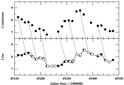
Figure 24: Continuum and emission-line light curves for Mrk 335, as in Fig. 23. This illustrates the interpolation method commonly used in cross-correlation. In this figure, the emission-line light curve is made continuous through linear interpolation between data points. Actual continuum observations are then paired with interpolated emission-line values to compute the correlation coefficient for a particular time delay. In this example, we show interpolated emission-line fluxes that are time-delayed relative to the continuum by 15.6 days, which is the value at which the cross-correlation function peaks. As a visual aid, dotted lines join a few of the data pairs. Notice how the first few points of the emission-line series and the last few points of the continuum series remain unused.

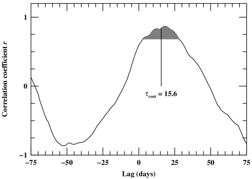
Figure 25: The interpolation cross-correlation function for the Mrk 335 data shown in the previous figures. The shaded area indicates points with values $r\geq 0.8r_{\rm peak}$, which are the points used in computing the centroid, which is also indicated.

4.2 Relationship to the Transfer Function

It is useful at this point to examine how the CCF is related to more fundamental quantities. Defined as a function of the continuous variable $\tau$, the formal definition of the cross-correlation function is

$${\rm CCF}(\tau)=\int^{\infty}_{-\infty}L(t)C(t-\tau)\ dt\mbox{\ \ .}$$ (32)

If we use Eq. (21) to replace $L(t)$ in this equation, we obtain

$${\rm CCF}(\tau) = \int^{\infty}_{-\infty}C(t-\tau)\int^{\infty}_{-\infty}\Psi(\tau^{\prime})C(t-\tau^{\prime})\ d\tau^{\prime}\ dt$$ (33)

$$= \int^{\infty}_{-\infty}\Psi(\tau^{\prime})\int^{\infty}_{-\infty}C(t-\tau^{\prime})C(t-\tau)\ dt\ d\tau^{\prime}\mbox{\ \ .}$$

Comparing the inner integral with Eq. (32), we see that it is the cross-correlation of the continuum light curve with itself, i.e., the “autocorrelation function”,

$${\rm ACF}(\tau)=\int^{\infty}_{-\infty}C(t)C(t-\tau)\ dt\mbox{\ \ .}$$ (34)

Thus, we see that the cross-correlation function is the convolution of the transfer function with the continuum autocorrelation function,

$${\rm CCF}(\tau)=\int^{\infty}_{-\infty}\Psi(\tau^{\prime}){\rm ACF}(\tau-\tau^{\prime})\ d\tau^{\prime}\mbox{\ \ .}$$ (35)

The centroid of the CCF is a usually quoted quantity,

$$\tau_{\rm cent}=\frac{\int\!\tau\,{\rm CCF}(\tau)\,d\tau}{\int{\rm CCF}(\tau)\ d\tau}\mbox{\ \ ,}$$ (36)

which is related to the centroid of the transfer function

$$\tau^{*}_{\rm cent}=\frac{\int\!\tau\,\Psi(\tau)\,d\tau}{\int\!\Psi(\tau)\ d\tau}\mbox{\ \ .}$$ (37)

It is important to note that these two quantities are the same only in the limit where the light curves extend to infinity. Operationally, the centroid is computed using only points around the most significant peak, usually those points for which ${\rm CCF}(\tau)\geq 0.8r_{\rm peak}$, where $r_{\rm peak}$ is the maximum value of the CCF. Sometimes the location of the peak $\tau_{\rm peak}$ (${\rm CCF}(\tau_{\rm peak})=r_{\rm peak}$) is the statistical quantity used.

Cross-correlation does not necessarily give a clean and unambiguous measure of the relationship between two time series. In particular, the CCF is a convolution of the transfer function with the continuum ACF, so the CCF depends on the continuum behavior. To illustrate this, we show in Fig. 26 examples of light curves for various power-law PDSs (Eq. (7)) and the very different ACFs computed for each example.

Figure 26: The left-hand column shows artificial light curves generated with different power-law indices $\alpha$ for the power-density spectra, $P(f)\propto f^{-\alpha}$. All light curves consist of 2048 points, normalized by setting $F_{\rm var}=0.3$ (Eq. (2)). The right-hand column shows the autocorrelation functions for these light curves. Cases shown, top to bottom, are: (a) $\alpha=0$. There is no correlation from one point to the next, as seen clearly in the ACF, which is essentially zero except at $\tau=0$. This is known as “white noise.” (b) $\alpha=1$. This is the power spectrum characteristic of a random walk; each continuum point now has some dependence on history. This case is sometimes called “flicker noise” (see Press⁷⁸ for further interesting discussion of this case). (c) $\alpha=1.5$. This appears to be rather typical of AGN variability. (d) $\alpha=2$. This power spectrum is characteristic of a superpositioning of independent events, which is often referred to as “shot noise.”

4.3 Discrete Correlation Methods

There are some circumstances under which one might not be able to reasonably interpolate between gaps in data. This can occur (a) when there are a few large gaps in otherwise well-sampled series or (b) when there is reason to believe that the variations might be at least somewhat undersampled. In these cases, interpolation might be highly misleading, and another methodology needs to be employed. The “discrete correlation function” (DCF)[20] method is one where no assumption about light curve behavior needs to be made. The DCF method deals with irregularly sampled data by binning the data in time, as illustrated schematically in Fig. 27. This is an alternative approach to the irregular sampling requirement: instead of requiring that points contributing to ${\rm CCF}(\tau)$ are separated in time by exactly the interval $\tau$, we time-bin the data by pairing points with time separations in the range $\tau\pm\Delta\tau/2$, where $\Delta\tau$ is the width of one time bin. Choice of the binning window is a free parameter, and two examples are shown in Fig. 28.

Figure 27: Part of the light curves from the previous figures, expanded to show DCF bins. The particular example shown is for a time-lag bin width $\Delta\tau=4$ days and shows the location of the bins, pairing real continuum points with emission-line points within a 4-day window, centered at a shift of 4 days (i.e., emission-line data points shifted by 2–6 days from the continuum points). Note that in this expanded region there are only three emission-line points that fall into the bins; in the range shown here, only two continuum and three emission-line points contribute to the computation of the correlation coefficient.

Figure 28: Cross-correlation functions for the Mrk 335 light curve shown in Fig. 23. The DCF values are shown as points with error bars, and the interpolation CCF, as in Fig. 25, is shown as a solid line. The upper panel shows the DCF with a bin width of $\Delta\tau=4$ days, and the lower panel shows a bin width of $\Delta\tau=8$ days; with $\Delta\tau=4$ days, some bins have no data (those with values set to $r=-1$), but with $\Delta\tau=8$ days, the DCF is somewhat underresolved.

The principal virtues of the DCF method are (a) that only actual data points are used and (b) that it is possible to assign a statistical uncertainty to the value of the correlation coefficient in each bin. The relative weakness of the DCF is that the data are in some ways underutilized, as is evident in Fig. 27; for a small data set, the DCF method might completely miss a real correlation, although it is less like to find a spurious correlation than is the interpolation method[94].

One difficulty of the DCF method is that the number of points per time bin can vary greatly, as can be easily inferred from inspection of Figs. 27 and 28. One solution to this is to vary the width of the time bins to ensure that there are a statistically meaningful number of points in each bin. A method for accomplishing this is the “Z-transformed DCF (ZDCF)”[1].

4.4 Computational Issues

In the foregoing discussion, we have concentrated primarily on conceptual issues without paying much attention to a number of computational issues that must be dealt with in actually computing CCFs[94]^,[92]^,[87].

1. Edge effects. Only at zero lag do all the points of the time series enter into the calculation of the correlation coefficient; at any other lag, points at the ends of the time series drop out of the calculation since there are no points in the other series to which they can be matched (see Fig. 24). This means that at larger and larger lags, fewer and fewer points contribute to the calculation of $r$. This has two significant consequences:

   1. Normalization. Correct normalization of the CCF requires use of the correct value of the mean and standard deviation for each series, as can be seen from the definition of the correlation coefficient $r$ (Eq. (31)). Since AGN time series are limited in duration, as points near the edges drop out of the calculation, the mean and standard deviation of the series change; in statistical language, this means that the series are “non-stationary.” Thus, the mean and standard deviation of the series needs to be recalculated for every lag, using only the data points that actually contribute to the calculation. In the case where interpolated values from one series are used, the mean and standard deviation should be those of the interpolated points, not the original points.

   2. Significance. Once the peak value of the CCF $r_{\rm peak}$ has been found, we want to know whether or not the correlation found is “statistically significant”, i.e., is it likely to be real or spurious? The statistical significance of the correlation depends on the number of points that contribute to the calculation of $r_{\rm peak}$, not to the total number of points in the series. Suppose, for example, that we have two time series consisting of $N=50$ points, but that the maximum value of the CCF (say, $r_{\rm peak}=0.45$) occurs at a such a large lag that only $N=30$ of the points are actually contributing at this lag. For a linear correlation coefficient of $r=0.45$ and $N=30$, the correlation is significant at about the 98% confidence level. However, if we erroneously use $N=50$, we would conclude that the level of significance is about 99.9%, clearly a major difference. If we fail to account for the correct number of points contributing to the calculation of $r_{\rm peak}$ and simply use the number of points in the series, we will overestimate the significance of the correlations we detect.

2. Interpolation scheme. There are a couple of issues that arise in this regard:

   1. Which series? In the examples shown in Fig. 24, we have interpolated in the emission-line light curve. Is there any particular reason to choose one series over the other when doing the interpolation? In general there does not seem to be, unless, for example, the emission-line light curve is markedly smoother than the continuum light curve (on account of the time-smearing effect) or one light curve is much better sampled than the other. Usually, one computes the CCF by computing the CCF twice, interpolating once in each series, and then averaging the results[28].

   2. Interpolating function. Here we have considered only point-to-point linear interpolation, which results in first-derivative discontinuities in the light curves and the CCFs. Is there any advantage to using higher-order interpolation functions in the time series? Generally, no, higher-order functions don’t improve the CCFs in any sense, and can be grossly misleading, as higher-order fits based on only a few data points become hard to control.

3. Resolution of the CCF. Can the accuracy of a cross-correlation result be better than the typical sampling interval? Yes, it can, as long as the functions involved are reasonably smooth. The analogy that is usually drawn is that one can measure image centroids to far higher accuracy than the image size, which is true because both stellar images and instrumental point-spread functions are generally smooth and symmetric. Statistical tests as described below suggest that uncertainties of about half the sampling interval are routinely obtained.

4.5 Uncertainties in Cross-Correlation Lags

Although cross-correlation techniques have been applied to AGN time series for about 15 years, there is still no obvious or even universally agreed-upon way to assess the uncertainties in the lag measurements obtained. At present, the most effective technique seems to be a model-independent Monte-Carlo method known as FR/RSS (for “flux redistribution/random subset selection”)[70].

FR/RSS is based on a computationally intensive statistical method known as a “bootstrap”. The bootstrap works as follows: suppose that you have a set of $N$ data pairs ($x_{i},y_{i}$) and that linear regression yields a correlation coefficient $r$. How accurate is $r$? In particular, how sensitive is it to the influence of individual points? One can assess this by a Monte Carlo process where one selects at random $N$ points from the original sample, without regard to whether or not any point has been selected previously. For the new sample of $N$ points (some of which are redundant selections from the original sample, while some points in the original sample are missing), the linear correlation coefficient is recalculated. When this is done many times, a distribution in $r$ is constructed, and from this, one can assign a meaningful statistical uncertainty to the original experimental value of $r$.

This process can also be assigned to time series, except that the time tags of the points have to be preserved. In effect, then, this means that redundant selections are overlooked; the probability that in $N$ selections of $N$ points a point will be selected zero times is $1/e$, so the new time series, selected at random, has typically fewer points by a factor of $1/e$ (hence the name “random subset selection”). Welsh[92] suggests that this should be modified in the sense that the weighting of each selected point should be proportional to $\sqrt{n_{i}}$, where $n_{i}$ is the number of times the data point $(x_{i},y_{i})$ is selected in a single realization. This is closer in philosophy to the original bootstrap, but it has not been rigorously tested yet.

The other part of the process, “flux redistribution,” consists of changing the actual observed fluxes in a way that is consistent with the measured uncertainties. Each flux is modified by a random Gaussian deviate based on the quoted error for that datum (i.e., after a large number of similar modifications, the distribution of flux values would be a Gaussian with mean equal to the data value and standard deviation equal to the quoted error).

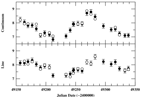
Figure 29: The filled circles show the Mrk 335 light curve from Fig. 23, but now with error bars shown. The open circles show a single FR/RSS Monte Carlo realization; the points are selected from the total subset at random, and the fluxes are adjusted as Gaussian deviates. Note that some of the original data points are not seen because the selected flux-adjusted points cover them. The realization shown here gives $\tau_{\rm cent}=17.9$ days, compared to $\tau_{\rm cent}=15.6$ days for the whole data set.

Figure 30: Multiple Monte-Carlo realizations such as those in Fig. 29 are used to build up a cross-correlation peak distribution (CCPD). Relative to the measured CCF centroid for the whole data set ($\tau=15.6$ days), the $\pm 1\sigma$ width of this distribution is $+7.2$, $-3.1$ days.

A single sample FR/RSS realization is shown schematically in Fig. 29. For each such realization, a cross-correlation is performed and the centroid is measured. A large number of similar realizations will produce a “cross-correlation peak distribution” (CCPD)[49], as shown in Fig. 30. The CCPD can be integrated to assign formal uncertainties (usually $\pm 1\sigma$) to the value of $\tau_{\rm cent}$ measured from the entire data set.

5 Observational Results

With the background provided in the previous sections, we can discuss some of the more important observational results. We will begin with emission-line variability, since the results obtained thus far have been relatively less ambiguous than the results on interband continuum variations.

5.1 Size of the Broad-Line Region

By the late 1980s, the potential power of reverberation mapping was widely understood, but the high-intensity monitoring programs required to extract this information had not been carried out, mainly on account of sociological barriers: the sampling requirements, in terms of time criticality and number of observations, were far in excess of anything that had been done in the past on oversubscribed shared facilities. In late 1987, a large informal consortium known as the International AGN Watch was formed in an attempt to obtain sufficient observing time with IUE and various ground-based observatories to measure emission-line lags for the Seyfert 1 galaxy NGC 5548, even at that time one of the best-studied variable AGNs. This turned out to be an enormously successful project[14]^,[66]^,[67] that provided impetus for additional similar projects by the AGN Watch and other groups (see Peterson[62] for a review of the field in the wake of the first monitoring project on NGC 5548). Some of the light curves and CCFs from the original NGC 5548 project are shown in Fig. 31.

Figure 31: Light curves (left-hand column) and CCFs (right-hand column) for NGC 5548, from the first International AGN Watch monitoring project in 1988–89. From the top, the light curves are the UV continuum at 1350 Å, the optical continuum at 5100 Å, He ii $\lambda 1640$, Ly$\alpha$ $\lambda 1215$, C iv $\lambda 1549$, C iii] $\lambda 1909$, and H$\beta$ $\lambda 4861$. The continuum fluxes are in units of $10^{-15}$ ergs s^-1 cm^-2 Å^-1, and the line fluxes are in units of $10^{-13}$ ergs s^-1 cm^-2. The CCFs are computed relative to the UV continuum at the top; the top panel is the UV continuum ACF. Data from Clavel et al.¹⁴ and Peterson et al.⁶⁷.

Since this initial successful campaign, a handful of AGNs have been well-monitored in the UV and optical (NGC 3783, NGC 4151, NGC 7469, 3C 390.3, Fairall 9, in addition to NGC 5548) and nearly three dozen Seyfert galaxies and low-luminosity quasars have been closely monitored in the optical[88]^,[36]. The most important general conclusions reached from these monitoring programs are:

1. The UV/optical continua vary together, to within a couple of days.

2. The highest ionization emission lines respond most rapidly to continuum changes, implying that there is ionization stratification of the BLR.

3. The BLR gas is not in pure radial motion, since no unambiguous differences in the time scale of the response of the blue and red wings of the emission lines have been detected.

Cross-correlation results show that the size of the H$\beta$-emitting region scales with average continuum luminosity as[36]

$$r({\rm H}\beta)\approx 0.22\left(\frac{L_{\rm bol}h_{0}^{2}}{10^{46}\,{\rm ergs\ s}^{-1}}\right)^{0.7}\ {\rm pc},$$ (38)

and that, in general, sizes derived from other lines usually scale as $r(\mbox{\rm He\,{\sc ii}, N\,{\sc v}})\approx 0.2r({\rm H}\beta)$ and $r(\mbox{\rm Ly$\alpha$, C\,{\sc iv}})\approx 0.5r({\rm H}\beta)$. A slightly different version of the BLR radius-luminosity relationship is shown in Fig. 32, in which $r\propto L^{0.6\pm 0.1}$. This is close to the slope of the relationship predicted by the most naive sort of scaling: since to lowest order AGN spectra all look alike, the ionization parameters (Eq. (13)) and particle densities must be the same in all of them. Thus, inverting Eq. (13), we predict that

$$r=\left(\frac{Q({\rm H})}{4\pi cn_{\rm e}}\right)^{1/2}\propto L^{1/2}\mbox{\ \ ,}$$ (39)

where in the last step we have also assumed that the shape of the ionizing continuum is not a function of luminosity. Despite these gross assumptions, the agreement with the data is not bad, although the large scatter alone tells us that this is not the whole story.

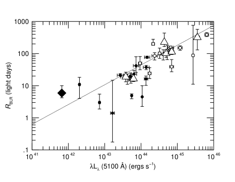
Figure 32: The BLR radius, as measured by the H$\beta$ lag, as a function of average optical continuum luminosity. The open symbols are Palomar–Green quasars from Kaspi et al.³⁶, the filled circles are Seyfert 1 galaxies from Wandel et al.⁸⁸. The large symbols are narrow-line ($V_{\mbox{\tiny FWHM}}<2000$ km s^-1) AGNs, and the filled diamond is NGC 4051⁷⁵. The dotted line is the best fit to all the data except NGC 4051.

5.2 AGN Black-Hole Masses

Reverberation mapping is one method of measuring AGN central masses via the virial relationship

$$M=\frac{fr\sigma^{2}}{G}\mbox{\ \ ,}$$ (40)

where $f$ is a dimensionless factor of order unity that depends on the geometry and kinematics of the BLR, $\sigma$ is the emission-line velocity dispersion, and $r$ is the size of the emitting region. Measurement of the emission-line time lags provides the ingredient that has been missing since the first attempts to understand the basic physics of AGNs[95]. Relative to other dynamical estimators, advantage of using the BLR to provide an estimate of the mass of the central source is that it is located very close to the central source (within $\sim 10^{3}R_{\rm grav}$), leaving little doubt that the central mass is in fact a black hole. On the other hand, the kinematics of the BLR are not yet understood (see below), and non-gravitational forces might have a strong effect on gas motions. For the virial method to be applicable, the BLR kinematics must be dominated by gravity. Even without understanding the detailed geometry and kinematics of the BLR, we can test the virial hypothesis by comparing lags and line widths measured in a single AGN: all lines must give the same virial mass, even though not all the line-emitting material needs to have common kinematics. The three AGNs for which this can be easily tested are shown in Fig. 33.

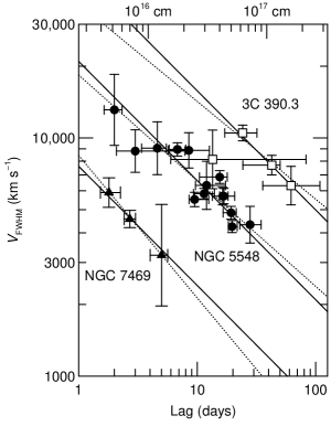
Figure 33: Line width in the rms spectrum plotted as a function of the distance from the central source (upper horizontal axis) as measured by the emission-line lag (lower horizontal axis) for various broad emission lines in NGC 7469, NGC 5548, and 3C 390.3. The dashed lines are best fits of each set of data to the relationship $\log V_{\mbox{\tiny FWHM}}=a+b\log c\tau$. The solid line shows the best fit to each set of data for fixed $b=-1/2$, yielding virial masses of $8.4\times 10^{6}\,{\rm M}_{\odot}$, $5.9\times 10^{7}\,{\rm M}_{\odot}$, and $3.2\times 10^{8}\,{\rm M}_{\odot}$ for the three respective galaxies. From Peterson & Wandel⁷² ©2000 AAS..

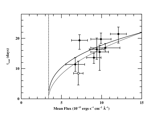
Figure 34: The H$\beta$ emission-line lag as a function of optical continuum flux for the Seyfert 1 galaxy NGC 5548. The solid line shows the best power-law fit to the data, $\tau\propto F^{0.4\pm 0.2}$, and the dotted line shows the best fit to the naive theoretical prediction $\tau\propto F^{1/2}$ (Eq. (39)). The dashed vertical line shows the estimated starlight contribution, as in Fig. 1.

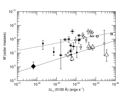
Figure 35: The central mass of AGNs, as measured from H$\beta$ line reverberation, as a function of optical continuum luminosity. Symbols are as in Fig. 32. From Peterson et al.⁷⁵ ©2000 AAS.

Even if this were not true for all lines, it may be true for some lines, and a given line must always yield the same mass. Only in the case of NGC 5548 is there sufficient information on the long-term behavior of a single line (H$\beta$) for this test to be applied, and the data seem to be consistent with the virial relationship[72]. We expect, then, that as the continuum brightens, the emission-line lag increases (see Fig. 34), and the emission-line becomes narrower. This does seem to be the case.

Virial masses based on H$\beta$ line reverberation as a function of optical luminosity are shown in Fig. 35. There is considerable scatter in the relationship, but it is nevertheless clear that higher-mass black holes are found in higher-luminosity AGNs. Some of the scatter in this relationship may be attributable to differences in accretion rate or radiative efficiency: the lower end of the envelope, for example, seems to be dominated by narrow-line Seyfert 1 galaxies, which are thought to have relatively high accretion rates (and thus luminosities) for their mass. Additional factors, such as inclination of the system, may also contribute to the scatter. But we are, finally, beginning to see the first indications of a mass-luminosity relationship for AGNs.

5.3 Emission-Line Transfer Functions

While existing AGN monitoring data have been of sufficient quality and quantity to obtain cross-correlation lags, recovery of transfer functions has, not surprisingly, proven to be far more difficult. Existing transfer function solutions tend to be very noisy and ambiguous.

In Fig. 36, we show a sample transfer function for the H$\beta$ emission line in NGC 5548; this transfer function is based on data extending over more than a crossing time, so the reader is cautioned against concluding too much from this example, since it is based on data that span a long interval compared to the BLR dynamical time scale (Eq. (19)). The structures seen in this transfer function do not correspond to those seen in any of the simple models that we have described earlier. Note in the one-dimensional transfer function the low amplitude of the response at zero lag, first noticed even with just the first year of AGN Watch data[34]; this indicates that there is little response due to material along our line-of-sight to the continuum source, suggestive of either a low-inclination disk (i.e., there is little gas along the line of sight) or anisotropic line response[24]. Whether or not other lines have small response at small lag is less certain[43]^,[62]; this effect may be seen clearly only in H$\beta$ on account of the large lag.

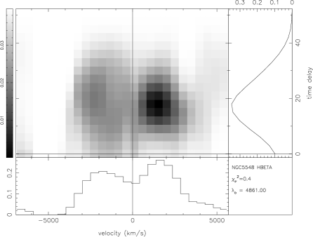
Figure 36: A transfer function for H$\beta$ in NGC 5548, based on AGN Watch data from 1988–1996. Courtesy of S. Collier.

Fig. 37 shows an attempt to recover the C iv transfer function from 39 daily observations of NGC 5548 made with HST in 1993. These data have been used in several independent analyses[90]^,[19]^,[11]^,[8] with no consensus on the interpretation, and indeed with quite contrary conclusions about the kinematics: Wanders et al.[90] favor no radial motion, Done & Krolik[19] find a hint of radial infall (also previously suggested by Crenshaw & Blackwell[18] on the basis of the first year of IUE data), and Chiang & Murray[11] and Bottorff et al.[8] fit the data with different radial-outflow models.

A crude measure of the velocity field might be obtained by cross-correlating parts of the emission line: for example, comparison of the response times for the red and blue wings could be used to detect radial infall/outflow. Similarly, one could compare the response times for the line wings with the line core in an attempt to detect virial motion, i.e., $V\propto r^{-1/2}$. There have been a number of reports that the emission lines wings respond faster than core[13], as expected for virial motion, but detection is always weak.

A two-dimensional transfer function for the C iv–He ii spectral region in NGC 4151 is shown Fig. 38. Ulrich & Horne[85] argue that there is a hint that the red wing responds slightly more rapidly than the blue wing, which is the expected signature for radial infall.

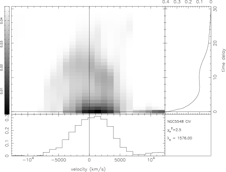
Figure 37: A transfer function for C iv $\lambda 1549$ in NGC 5548, HST observations⁴⁰ from 1993. Courtesy of S. Collier.

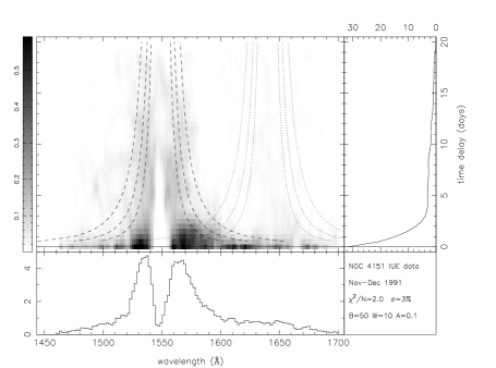
Figure 38: A transfer function for the C iv–He ii region of NGC 4151 based on IUE spectra. The strong double-peaked appearance of the C iv line is due to a deep slightly blueshifted absorption feature in this line. From Ulrich & Horne⁸⁵ ©1996 Blackwell Sci.

5.4 Emission-Line Profile Variability

If the BLR velocity field is ordered (i.e., $V=f(r)$), then the emission-line profiles should vary in response to continuum changes: the propagation of excitation inhomogeneities through the BLR should result in irregularities in line profiles that evolve on time scales comparable to the emission-line lags. Peterson et al.[73] have examined profile variations in several Seyfert galaxies that were monitored fairly intensively over several years. They conclude that profile variations are not obviously correlated with either the continuum or the total emission-line flux; profile variations are not reverberation effects. They also find that most H$\beta$ profiles can be modelled fairly well with three Gaussian components that are fixed in location and width and vary only in relative flux, which thus allows multiple-peaked profiles and variable asymmetry. They also conclude that profile irregularities can occur quickly, appearing on time scales as short as days or weeks, but they can then persist for a very long time, months or even years. Sample H$\beta$ profiles for two well-studied Seyferts are shown in Fig. 39.

Figure 39: Emission-line profiles for H$\beta$ in NGC 5548 (left-hand column; International AGN Watch data) and Akn 120 (right-hand column; data from Peterson et al.⁶⁹). These are representative profiles obtained over several years of monitoring. The H$\beta$ narrow-line component is particularly noticeable in the spectra of NGC 5548.

5.5 Multiwavelength Continuum Variability

As noted earlier, one of the important conclusions reached from the original AGN Watch monitoring program was that the UV and optical continua vary with no apparent time delay between them, at least to the accuracy of the experiment ($\raisebox{-2.15277pt}{$\;\stackrel{{\scriptstyle<}}{{\sim}}\;$}1$ day in the best cases). An important consequence of this is that AGN continuum variability is not due either to mechanical accretion-disk instabilities or to variations in the accretion rate, since such effects would be expected to propagate through the disk (and thus across the spectrum) on much-longer sound-crossing (Eq. (11)) or drift time scales (Eq. (12)), respectively. The suggestion was made[17]^,[15] that the UV/optical variations might in fact be driven by X-ray variations, possibly in a manner consistent with the X-ray reprocessing models that were being developed to account for the 10 keV reflection hump and the equivalent width of the 6.4 keV Fe K$\alpha$ line[32]^,[46]^,[29]; both of these features suggest that something like half of the emitted hard X-rays in AGN interact with “cold” (not highly ionized) matter that covers much of the sky as seen from the source (and which might in fact be the accretion disk itself). If it is supposed that hard X-rays are produced above the disk plane near the axis of the accretion disk, then hard X-ray radiation striking the disk should be reprocessed into lower-energy continuum photons. Moreover, the UV/optical variations should follow those in the X-rays, with the shortest time delays for the higher-energy photons that are produced predominantly in the central regions of the accretion disk. The temperature structure of a classical thin accretion disk is given by

$$T^{4}=\frac{3GM\dot{M}}{8\pi\sigma r^{3}}\left[1-\left(\frac{r}{R_{\rm min}}\right)^{-1/2}\right]\mbox{\ \ ,}$$ (41)

and assuming that AGNs are accreting close to the Eddington rate with about 10% efficiency, the radial temperature structure becomes

$$T(r)\approx 6.3\times 10^{5}\left(\frac{\dot{M}}{\dot{M}_{\rm Edd}}\right)^{1/4}\left(\frac{M}{10^{8}\,{\rm M}_{\odot}}\right)^{-1/4}\left(\frac{r}{R_{\rm S}}\right)^{-3/4}\ {\rm K}\mbox{\ \ ,}$$ (42)

from which we expect a peak in the spectral energy distribution in the UV/soft X-ray region, which as noted earlier might in fact be the origin of the big blue bump[81]^,[48].

If we suppose that a thin accretion disk is irradiated by an X-ray source on the disk axis, we should see the inner, hotter part of the accretion disk respond before the outer, cooler parts. From Wien’s Law, the radiation at wavelength $\lambda$ arises primarily at a particular temperature corresponding to a particular location in the disk, i.e., $\lambda\propto T^{-1}\propto r^{3/4}$, so the difference in the response times at different wavelengths should be naively

$$\Delta\tau\propto\lambda^{4/3}\mbox{\ \ .}$$ (43)

It is straightforward to show that this relationship holds for an irradiated disk that is heated locally by hard X-rays.

The predicted wavelength-dependent continuum time delays have been detected reliably in the case of NGC 7469, which was monitored intensively in 1996[91]^,[16]^,[42]. Fig. 40 shows the result of measuring the UV and optical fluxes across the entire monitored UV and optical spectrum, and cross-correlating each of the resulting light curves with the shortest-wavelength UV continuum. Relative to the short-wavelength UV, continuum lags in other line-free continuum bands are detected at no less than 97% confidence throughout the UV/optical region.

Figure 40: Lag as a function of wavelength for NGC 7469. The average flux in each wavelength band is cross-correlated with the shortest-wavelength UV (1315 Å) continuum, yielding a “lag spectrum”. The expected dependence for an irradiated thin accretion disk, $\tau\propto\lambda^{4/3}$, is also shown. The broad emission lines are prominent because they have longer response times than the adjacent continuum.

While the evidence shows that there are in fact wavelength-dependent continuum lags in NGC 7469, this is not an unambiguous detection of a classical thin accretion-disk structure. There are several complications:

1. Similar wavelength-dependent lags have not been reliably detected in other sources. This effect may be marginally present in the case of NGC 4151[70], but it is not found in NGC 3516[22]. However, the sampling rates obtained for NGC 7469 are far superior to those of most other experiments, and the upper limits on UV/optical continuum lags for other AGNs seem to be consistent with predictions based on (highly uncertain) scaling of the other sources to the NGC 7469 result, except possibly in the case of NGC 3516.

2. Korista & Goad[41] have suggested wavelength-dependent lags are consistent with the expectations for diffuse emission from the emission-line clouds (Balmer and Paschen continuum). Observations over a wider wavelength range are needed to distinguish between an accretion-disk and a diffuse-continuum origin (specifically, the NGC 7469 observations did not cover the crucial wavelength range around the Balmer edge $\sim 3650$ Å).

3. The hard X-ray flux variations in NGC 7469 are not correlated with those in the UV/optical[57]. The hard X-ray spectrum was monitored with RXTE at the same time as the UV/optical monitoring campaign. Comparison of the light curves shows that the minima occurred at about the same time, but the hard X-ray maxima occurred approximately 4 days later than the corresponding maxima in the UV continuum light curve. This is a prima facie argument against the reprocessing scenario. However, a more complete spectral analysis[56] enabled by an improved background model for RXTE finds that the UV flux variations are correlated with variations in the X-ray spectral index, in the sense that the X-ray spectrum is softer when the UV is brighter. This suggests that the soft X-rays are strongly correlated with the UV; an increase in the number of UV seed photons cools the Comptonizing corona above the accretion disk, softening the spectrum.

By way of contrast, a recent study of high-energy variability in NGC 5548 shows clear relationships between the hard X-rays and the lower-energy photons[12]: the extreme ultraviolet (EUV) variations lead those in the soft X-ray region by about 3.5 hrs and those in the hard X-ray by about 10 hrs. The temporal order and time scales are consistent with production of both the soft and hard X-rays by Compton upscattering of lower-energy photons.

If the X-rays are indeed Comptonized lower-energy photons, are the seed photons in the EUV ($\sim 100$ Å) or UV ($\sim 1000$ Å)? The only good comparison available is based on simultaneous UV and EUV monitoring of NGC 5548 in 1993[50]. Cross-correlation of the UV and EUV light curves shows that the UV leads, with $\tau_{\rm cent}=0.1^{+0.7}_{-0.2}$ days, which is consistent with zero lag and leaves the question unanswered.

Figure 41: Comparison of hard X-ray and optical spectral variations in NGC 4051 in different X-ray states. Panel (a) shows the 2–10 keV flux measured with RXTE as a function time for the three-year period 1996–1998. Panel (b) shows the rms optical spectrum during an X-ray active period in 1996, Panel (c) shows the rms optical spectrum during an X-ray quiescent period in 1998. Note the absence of strong He ii $\lambda 4686$ emission in panel (c). From Peterson et al.⁷⁵ ©2000 AAS.

A final recent observation that should be mentioned is based on a three-year combined X-ray (RXTE) and optical monitoring program on the narrow-line Seyfert 1 galaxy NGC 4051[75]. During the first two years of this program, NGC 4051 behaved in a “normal” fashion for narrow-line Seyfert 1s, with rapid, violent X-ray variability and much lower-amplitude optical variations. During the third year, NGC 4051 went into a very low X-ray state. In Fig. 41, the top panel shows the X-ray light curve. The bottom two panels show rms optical spectra, which isolate the variable parts of the spectrum, obtained during the two periods indicated, one during a high X-ray state and one during the low X-ray state. They are remarkably different. The high-state rms spectrum (lower left) shows that the optical continuum and the H$\beta$ and He ii $\lambda 4686$ emission lines were all varying strongly. However, the low-state rms spectrum (lower right) shows that the optical continuum and the H$\beta$ emission line are still present and variable, but the He ii line has vanished from the rms spectrum, meaning that it is absent or constant. Whether or not it has completely vanished is difficult to determine on account of the blending of He ii with strong Fe ii emission in the mean spectrum, but an attempt to remove the Fe ii emission by subtraction of a template indicates that most of the He ii emission must have vanished during 1998. This indicates that not only has the X-ray flux dramatically decreased, but the EUV flux (which drives the He ii variations) must have also decreased by a significant amount. This may suggest that the entire inner accretion disk has undergone a transition to a low-radiation state, such as an “advection-dominated accretion flow” [57].

5.6 Conclusion

The few examples cited in this section give an indication of the power of coordinated multiwavelength observations for understanding the physical mechanisms at work in AGNs on angular scales far too small to be resolvable with any current or near-term technology. These are difficult programs to implement, but the scientific return on them is potential very large, especially as we can build on the significant progress that has already been made.

References

- [1] Alexander T., in Astronomical Time Series, ed. D. Maoz, A. Sternberg, & E.M. Leibowitz (Dordrecht: Kluwer), p. 163, 1997.
- [2] Andrillat Y., & Souffrin S., Ap. Lett., 1, 111, 1968.
- [3] Antokhin I.I., & Bochkarev N.G., Soviet Astr., 27, 261, 1983.
- [4] Antonucci R.R.J., & Cohen R.D., ApJ, 271, 564, 1983.
- [5] Bahcall J.N., Kozlovsky B.-Z., & Salpeter E.E., ApJ, 171, 467, 1972.
- [6] Bevington P.R., Data Reduction and Error Analysis for the Physical Sciences, (New York: McGraw–Hill), 1969.
- [7] Blandford R.D., & McKee C.F., ApJ, 255, 419, 1982.
- [8] Bottorff M., Korista K.T., Shlosman I., & Blandford R.D., ApJ, 479, 200, 1997
- [9] Bracewell R., The Fourier Transform and Its Applications, (New York: McGraw–Hill), p. 108, 1965
- [10] Capriotti E.R., Foltz C.B., & Peterson B.M., ApJ, 261, 35, 1982.
- [11] Chiang J., & Murray N., ApJ, 466, 704, 1996.
- [12] Chiang J., Reynolds C.S., Blaes O.M., Nowak M.A., Murray N., Madejski G., Marshall H.L., & Magdziarz P., ApJ, 528, 292, 2000.
- [13] Clavel J., in Variability of Active Galactic Nuclei, ed. H.R. Miller & P.J. Wiita (Cambridge: Cambridge Univ. Press), p. 301, 1991.
- [14] Clavel J., et al., ApJ, 366, 64, 1991.
- [15] Clavel J., Nandra K., Makino F., Pounds K.A., Reichert G.A., Urry C.M., Wamsteker W., Peracaula-Bosch M., Stewart G.C., & Otani C., ApJ, 393, 113, 1992.
- [16] Collier S., et al., ApJ, 500, 162, 1998.
- [17] Collin-Souffrin S., A&A, 249, 344, 1991.
- [18] Crenshaw D.M., & Blackwell J.H. Jr., ApJL, 358, L37, 1990.
- [19] Done C., & Krolik J.H., ApJ, 463, 144, 1996.
- [20] Edelson R.A., & Krolik J.H., ApJ, 333, 646, 1988.
- [21] Edelson R., & Nandra K., ApJ, 514, 682, 1999.
- [22] Edelson R., et al., ApJ, 534, 180, 2000.
- [23] Fabrika S.N., Soviet Astr. Lett., 6, 293, 1980.
- [24] Ferland G.J., Peterson B.M., Horne K., Welsh W.F., & Nahar S.N., ApJ 387, 95, 1992.
- [25] Fitch W., Pacholczyk A.G., & Weymann R.J., ApJL, 150, L67, 1967.
- [26] Foltz C.B., Peterson B.M., Capriotti E.R., Byard P.L., Bertram R., & Lawrie D.G., ApJ, 250, 508, 1981.
- [27] Gaskell C.M., & Sparke L.S., ApJ, 305, 175, 1986.
- [28] Gaskell C.M., & Peterson B.M., ApJS, 65, 1, 1987.
- [29] George I.M., & Fabian A., MNRAS, 249, 352, 1991.
- [30] Goad M.R., O’Brien P.T., & Gondhalekar P.M., in Reverberation Mapping of the Broad-Line Region in Active Galactic Nuclei, ed. P.M. Gondhalekar, K. Horne, and B.M. Peterson (Astronomical Society of the Pacific, San Francisco), p. 315, 1994.
- [31] Goad M., & Wanders I., ApJ, 469, 113, 1996.
- [32] Guilbert P.W., & Rees M.J., MNRAS, 233, 475, 1988.
- [33] Horne K., in Reverberation Mapping of the Broad-Line Region in Active Galactic Nuclei, ed. P.M. Gondhalekar, K. Horne, and B.M. Peterson (Astronomical Society of the Pacific, San Francisco), p. 23, 1994.
- [34] Horne K., Welsh W.F., & Peterson B.M., ApJL, 367, L5, 1991.
- [35] Hummer D.G., & Kunasz P.B., ApJ, 236, 609, 1980.
- [36] Kaspi S., Smith P.S., Netzer H., Maoz D., Jannuzi B.T., & Giveon U., ApJ, 533, 631, 2000.
- [37] Kawaguichi T., Mineshige S., Machida M., Matsumoto R., & Shibata K., PASJ, 52, L1, 2000.
- [38] Kollatschny W., Fricke K.J., Schleicher H., & Yorke H.W., A&A, 102, L23, 1981.
- [39] Koratkar A.P., & Gaskell C.M., ApJS, 75, 719, 1991.
- [40] Korista K.T., et al., ApJS, 97, 285, 1995.
- [41] Korista K.T., & Goad M.R., in Probing the Physics of Active Galactic Nuclei by Multiwavelength Monitoring, ed. B.M. Peterson, R.S. Polidan, & R.W. Pogge (San Francisco: Astronomical Society of the Pacific), in press.
- [42] Kriss G.A., Peterson B.M., Crenshaw D.M., & Zheng W., ApJ, 535, 58, 2000.
- [43] Krolik J.H., Horne K., Kallman T.R., Malkan M.A., Edelson R.A., & Kriss G.A., ApJ, 371, 541, 1991.
- [44] Krolik J.H., & Done C., ApJ, 440, 166, 1995.
- [45] Kwan J., & Krolik J.H., ApJ, 250, 478, 1981.
- [46] Lightman A.P., & White T.R., ApJ, 335, 57, 1988.
- [47] Madejski G.M., Done C., Turner T.J., Mushotzky R.F., Serlemitsos P., Fiore F., Sikora M., & Begelman M.C., Nat, 365, 626, 1993.
- [48] Malkan M.A., & Sargent W.L.W., ApJ, 254, 122, 1982.
- [49] Maoz D., & Netzer H., MNRAS, 236, 21, 1989.
- [50] Marshall H.L., et al., ApJ, 479, 222, 1997.
- [51] Matthews T.A., & Sandage A.R., ApJ, 138, 30, 1963.
- [52] McHardy I., Mem. Soc. Astron. Ital., 59, 239, 1988.
- [53] Mittaz J.P.D., & Branduardi-Raymont G., MNRAS, 238, 1029, 1989.
- [54] Mushotzky R.F., Done C., & Pounds K.A., ARAA, 31, 717, 1993.
- [55] Nandra K., Clavel J., Edelson R.A., George I.M., Malkan M.A., Mushotzky R.F., Peterson B.M., & Turner T.J., ApJ, 505, 594, 1998.
- [56] Nandra K., Le T., George I.M., Edelson R.A., Mushotzky R.F., Peterson B.M., & Turner T.J., ApJ, in press.
- [57] Narayan R., Mahadevan R., Grindlay J.E., Popham R.G., & Gammie C., ApJ, 492, 554, 1998.
- [58] Netzer H., & Peterson B.M., in Astronomical Time Series, ed. D. Maoz, A. Sternberg, & E.M. Leibowitz (Dordrecht: Kluwer), p. 85, 1997.
- [59] Osterbrock D.E., Astrophysics of Gaseous Nebulae and Active Galactic Nuclei (Mill Valley: University Science Books), 1989.
- [60] Pérez E., Robinson A., & de la Fuente L., MNRAS, 256, 103, 1992.
- [61] Peterson B.M., PASP, 100, 18, 1988.
- [62] Peterson B.M., PASP, 105, 247, 1993.
- [63] Peterson B.M., An Introduction to Active Galactic Nuclei, (Cambridge: Cambridge University Press), 1997.
- [64] Peterson B.M., Foltz C.B., Miller H.R., Wagner R.M., Crenshaw D.M., Meyers K.A., & Byard P.L., AJ, 88, 926, 1983
- [65] Peterson B.M., Meyers K.A., Capriotti E.R., Foltz C.B., Wilkes B.J., & Miller H.R., ApJ, 292, 164, 1985.
- [66] Peterson B.M., et al., ApJ, 368, 119, 1991.
- [67] Peterson B.M., et al., ApJ, 392, 470, 1992.
- [68] Peterson B.M., Pogge R.W., Wanders I., Smith S.M., & Romanishin W., PASP, 107, 579, 1995.
- [69] Peterson B.M., Wanders I., Bertram R., Hunley J.F., Pogge R.W., & Wagner R.M., ApJ, 501, 82, 1998.
- [70] Peterson B.M., Wanders I., Horne K., Collier S., Alexander T., & Kaspi S., PASP, 110, 660, 1998.
- [71] Peterson B.M., et al., ApJ, 510, 659, 1999.
- [72] Peterson B.M., & Wandel A., ApJL, 521, L95, 1999.
- [73] Peterson B.M., Pogge R.W., & Wanders I., in Structure and Kinematics of Quasar Broad-Line Regions, ed. C.M. Gaskell, W.N. Brandt, M. Dietrich, D. Dultzin-Hacyan, & M. Eracleous (San Franciso: Astronomical Society of the Pacific), p. 41, 1999.
- [74] Peterson B.M., & Wandel A., ApJL, 540, L13, 2000.
- [75] Peterson B.M., et al., ApJ, 542, 161, 2000.
- [76] Phillips M.M., ApJS, 38, 187, 1978.
- [77] Pijpers F.P., & Wanders I., MNRAS, 271, 183, 1994.
- [78] Press W., Comments on Ap., 7, 103, 1978.
- [79] Reynolds C.S., in Probing the Physics of Active Galactic Nuclei by Multiwavelength Monitoring, ed. B.M. Peterson, R.S. Polidan, & R.W. Pogge, (San Francisco: Astronomical Society of the Pacific), in press
- [80] Schulz H., & Rafanelli R., A&A, 103, 216, 1981.
- [81] Shields G.A., Nat, 272, 706, 1978.
- [82] Smith H.J., & Hoffleit D., Nat, 198, 650, 1963.
- [83] Tohline J.E., & Osterbrock D.E., ApJL, 210, L117, 1976.
- [84] Ulrich M.-H., Boksenberg A., Bromage G., Clavel J., Elvius A., Penston M.V., Perola G.C, & Snijders M.A.J., ApJ, 382, 483, 1991.
- [85] Ulrich M.-H., & Horne K., MNRAS, 283, 748, 1996.
- [86] Ulrich M.-H., Maraschi L., & Urry M., ARAA, 35, 445, 1997.
- [87] Vio R., & Wamsteker W.W., PASP, in press
- [88] Wandel A., Peterson B.M., & Malkan M.A., ApJ, 526, 579, 1999.
- [89] Wanders I., Peterson B.M., Pogge R.W., DeRobertis M.M., & van Groningen E., A&A, 266, 72, 1992.
- [90] Wanders I., Goad M.R., Korista K.T., Peterson B.M., Horne K., Ferland G.J., Koratkar A.P., Pogge R.W., & Shields J.C., ApJ, 453, L87, 1995.
- [91] Wanders I., et al., ApJS, 113, 69, 1997.
- [92] Welsh W.F., PASP, 111, 1347, 2000.
- [93] Welsh W.F., & Horne K., ApJ, 379, 586, 1991.
- [94] White R.J., & Peterson B.M., PASP, 106, 879, 1994.
- [95] Woltjer L., ApJ, 130, 38, 1959.