GALACTIC POPULATIONS OF RADIO AND GAMMA-RAY PULSARS IN THE POLAR CAP MODEL

Abstract

We simulate the characteristics of the Galactic population of radio and $\gamma$-ray pulsars using Monte Carlo techniques. At birth, neutron stars are spatially distributed in the Galactic disk, with supernova-kick velocities, and randomly dispersed in age back to $10^{9}$ years. They are evolved in the Galactic gravitational potential to the present time. From a radio luminosity model, the radio flux is filtered through a selected set of radio-survey parameters. $\gamma$-ray luminosities are assigned using the features of recent polar cap acceleration models invoking space-charge-limited flow, and a pulsar death valley further attenuates the population of radio-loud pulsars. Assuming a simple emission geometry with aligned radio and $\gamma$-ray beams of 1 steradian solid angle, our model predicts that EGRET should have seen 7 radio-loud and 1 radio-quiet, $\gamma$-ray pulsars. With much improved sensitivity, GLAST, on the other hand, is expected to observe 76 radio-loud and 74 radio-quiet, $\gamma$-ray pulsars of which 7 would be identified as pulsed sources. We also explore the effect of magnetic field decay on the characteristics of the radio and $\gamma$-ray pulsar populations. Including magnetic field decay on a timescale of 5 Myr improves agreement with the radio pulsar population and increases the predicted number of GLAST detected pulsars to 90 radio-loud and 101 radio-quiet (9 pulsed) $\gamma$-ray pulsars. The lower flux threshold allows GLAST to detect $\gamma$-ray pulsars at larger distances than those observed by the radio surveys used in this study.

1 Introduction

With the advent of the Compton Gamma Ray Observatory (CGRO), the number of $\gamma$-ray pulsars has grown to eight, with several additional candidates. We anticipate that many more pulsed sources will be added to the list with the future telescope, Gamma-Ray Large Area Space Telescope (GLAST) scheduled for launch in 2006. The new body of data with a much larger set of statistics will be essential in further constraining pulsar models. Many questions, such as the mechanism for radio emission and its relationship to $\gamma$-ray emission, and the location and geometry of the $\gamma$-ray emission currently remain unanswered. Among the known $\gamma$-ray pulsars, only Geminga is radio-quiet or at least radio weak (Kuzmin & Losovsky 1997 and Malofeev & Malov 1997). Geminga does not emit conventional radio emission that is detectable through the current radio surveys. As a result, we refer to this object as a radio-quiet, $\gamma$-ray pulsar. Of the 271 sources listed in the Third EGRET Catalog (Hartman et al. 1999), about 170 of these $\gamma$-ray point sources have not been identified with sources at other wavelengths. Recently Grenier & Perrot (1999) suggested that some of these unidentified sources are correlated with the Gould Belt of massive stars from a nearby Galactic structure consisting of an expanding disk of gas with young stars ($\leq$ 30 million years) inclined about $20^{o}$ to the Galactic plane. Gehrels et al. (2000) found that the flux distribution of 120 steady sources suggests two distinct groups: one having higher flux, hard spectra and distributed along the Galactic plane, and the other having lower flux, softer spectra and correlated with the Gould Belt. The soft spectra and luminosity of this second group of sources are significantly different than those of the known $\gamma$-ray pulsars observed by EGRET. Harding & Zhang (2001) suggest that some of the sources associated with the Gould Belt are indeed radio-quiet, off-beam $\gamma$-ray pulsars seen at large angles to the magnetic pole.

There are two main types of models proposed to explain pulsar high-energy emission. Polar cap models (Daugherty & Harding 1996, Sturner et al. 1995) assume that particles accelerated above the neutron star polar caps produce $\gamma$-rays via curvature radiation or inverse Compton scattering induced pair cascades in a strong magnetic field. Outer gap models (Cheng, Ho & Ruderman 1986, Romani 1996, Hirotani & Shibata 1999) assume that acceleration occurs along null charge surfaces in the outer magnetosphere and that $\gamma$-rays result from photon-photon pair cascades. Polar cap and outer gap models predict different ratios of radio-loud to radio-quiet, $\gamma$-ray pulsars, primarily due to the different geometry of the high-energy emission region and its location relative to the radio emission region, thought to originate within tens of stellar radii of the neutron star surface.

Outer gap models generally predict small overlap of the radio and high-energy pulsar populations, because the high-energy and radio pulses that are visible to the same observer originate from opposite magnetic poles, and large numbers of radio-quiet, $\gamma$-ray pulsars, because the outer gap beam is much larger than the radio beam. The study of Yadigaroglu & Romani (1995), using the outer gap model of Romani & Yadigaroglu (1995), found that EGRET should have detected about three times as many radio-quiet pulsars as radio-loud pulsars in $\gamma$ rays. Most of the pulsar population should be seen only in $\gamma$ rays, as Geminga-like pulsars. The Monte-Carlo simulation of Cheng & Zhang (1998) found that only about $16\%$ of radio pulsars should be $\gamma$-ray pulsars. They expect 55 Geminga-like pulsars to have been detected by EGRET, about all of the unidentified sources in the Galactic plane, as compared to 11 radio-loud $\gamma$-ray pulsars expected. The characteristics of the $\gamma$-ray pulsar population, as seen by EGRET, in the inverse-Compton initiated polar cap cascade model have been studied by Sturner & Dermer (1996a). They predict that about $75\%$ of radio-selected pulsars should be $\gamma$-ray pulsars but that only $25\%$ of $\gamma$-ray pulsars are radio-quiet. Although the uncertainties in these studies are large, it is apparent that the differences between expected populations of polar cap and outer gap models are larger than the uncertainties due to model-dependent effects.

Since there has been no statistical study of the expected high-energy pulsar populations in the curvature radiation-induced polar cap cascade model (e.g. Daugherty & Harding 1996), we have developed a Monte-Carlo code similar to that of Sturner & Dermer (1996a) to simulate the radio and $\gamma$-ray pulsar populations in the Galaxy. While we understand that the emission geometry is crucial to the modeling of the $\gamma$-ray pulsar population, we present in this study a simple geometric model that provides insight into the number of radio-loud and radio-quiet, $\gamma$-ray pulsars detected by EGRET and those expected to be detected by GLAST. The simplest geometric assumption suggested by the polar cap model is one in which the radio and the $\gamma$-ray beams are aligned and equal in solid angle. With this assumption, we model the population of radio and $\gamma$-ray pulsars in the Galaxy. We do not attempt to fit the observations. Rather we use standard distribution functions, evolution techniques, radio luminosity models and recent $\gamma$-ray luminosity models suggested by an acceleration-cascade model of the polar cap (Zhang & Harding 2000). The simple model presented in this paper predicts a ratio of radio-quiet to radio-loud, $\gamma$-ray pulsars (1/7) that is comparable to the one observed by EGRET (1/8). With a greater sensitivity, GLAST is expected to observe a ratio of 74/76. The large increase in the ratio of radio-quiet to radio-loud, $\gamma$-ray pulsars is due to the greater sensitivity of GLAST to detect $\gamma$-ray pulsars at greater distances from the Earth than the radio surveys used in this study. We plan to have forthcoming the logical extension of this work that will invoke more realistic emission geometries for both radio and $\gamma$-ray beams.

2 Monte Carlo Simulation Model

We develop a model to simulate the production of neutron stars within the Galaxy, evolving their trajectories, periods and period derivatives from their birth forward in time to the present. We supply the radio and $\gamma$-ray characteristics to each neutron star and filter its properties through radio surveys and $\gamma$-ray thresholds (in and out of plane) associated with EGRET and expected for GLAST. These $\gamma$-ray thresholds correspond to the number of photons required for the instrument to identify the object as a point source. Higher thresholds would be required to obtain sufficient photons to identify the object independently as a pulsed source.

2.1 Initial Pulsar Period and Magnetic Field

In most of our simulations, the magnetic field of the pulsar is assumed to be constant throughout its lifetime, although we also will explore the effect of field decay. A constant field requires that $(\dot{P}P)^{1/2}$ is equal to a constant and, therefore, implies a nonzero $\ddot{P}$. Following Bhattacharya et al. (1992) and Gunn & Ostriker (1970), we have assumed that the magnetic field distribution can be represented by a Gaussian. However, we found it necessary to include two additional Gaussians below the main distribution to account more fully for the inferred distribution from the period and period derivative of observed pulsars. The pulsar’s surface magnetic field distribution is represented by the expression

$$\rho{{}_{B}}=\sum\limits_{i=1}^{3}{A_{i}e^{-\left({\log B-\log B_{i}}\right)^{2}/\sigma_{i}^{2}}},$$ (1)

where the parameters take on the following values:

		Table 1
i	$A_{i}$	$\log(B_{i})$	$\sigma_{i}$
1	60.	12.65	0.45
2	2.	11.9	0.6
3	.001	10.4	4

An array normalized to unity is created with this distribution from $\log(B)=9.5$ to 13.5 in steps of 0.02, and used to randomly select the pulsar’s initial magnetic field.

The birth rate of neutron stars is assumed to be constant during the history of the Galaxy. Therefore, the age of the pulsar is randomly selected from the present to $10^{9}$ years in the past. While most of the very old pulsars will not be observed due to their very long periods, there will be some observed with ages close to $10^{9}$ years as a result of their small magnetic fields and, therefore, small period derivatives. We use the expression by Shapiro & Teukolsky (1983) and Usov & Melrose (1995) for a uniformly magnetized neutron star where the inferred magnetic field is given by the star-centered dipole relation, with magnetic moment $\mu=B_{0}R^{3}/2$,

$$B_{12}=6.4\ \times\ 10^{7}(P\dot{P}\ )^{1/2},$$ (2)

where $B_{12}$ is in units of $10^{12}$ Gauss. This relation is not used in the pulsar catalog by Taylor, Manchester & Lyne (1993) and in Lyne & Graham-Smith (1998) who instead use the approximate magnetic dipole moment, $\mu=B_{0}R^{3}$. Therefore, we multiplied the magnetic fields in the pulsar catalog by a factor of 2 in order to make comparisons. Integrating this expression over time results in a pulsar period in seconds at the present time by the expression:

$$P(t)=\left[{P_{o}^{2}+1.54\times 10^{-8}B_{12}^{2}t}\right]^{1/2},$$ (3)

where $t$ is the age of the pulsar in years and the initial period $P_{o}$ is in seconds. The initial period of the pulsar at birth is assumed to be a fixed 30 ms. The simulated distributions are rather insensitive to the initial period as long as $P_{o}\lower 2.0pt\hbox{$\,\buildrel\scriptstyle<\over{\scriptstyle\sim}\,$}100$ ms. Having the $P(t)$ along with the pulsar’s magnetic field, the pulsar’s period derivative can be obtained assuming a braking index of 3 from equation (2). Various studies (for example, Lyne, Pritchard & Smith 1988, Kaspi et al. 1994, and Boyd et al. 1995) measuring the second period derivative suggest a lower braking index. However, systematics are difficult to obtain as second derivatives of pulsar periods are very time consuming to measure. At this time, we have not attempted to model anything other than a braking index of 3.

Using the recent study of Zhang, Harding & Muslimov (2000), we have introduced a pulsar death line predicted by a multipole magnetic field configuration near the stellar surface within a space-charge-limited flow model and described by the expression

$$\log\dot{P}=2\log P-16.52.$$ (4)

The model includes the effect of general relativistic frame-dragging discussed in Muslimov & Tsygan (1992) and Muslimov & Harding (1997) essential in the development of the electric field parallel to the magnetic field. A more recent study of Harding & Muslimov (2001) has shown that the death line described by equation (4) roughly defines the boundary of pair production for a dipole field when non-resonant and resonant inverse Compton radiation processes are considered. Only pulsars with period derivatives greater than those of equation (4) are further considered.

In addition to the death line, we have introduced a death valley in the $\dot{P}-P$ space. Otherwise, we find too many pulsars are predicted near the death line that are clearly not present in the observed distribution. In order to define the death valley, we have used a second line from Zhang, Harding & Muslimov (2000) that describes the death line in the space-charged-limited flow model for a purely dipole magnetic field near the stellar surface given by

$$\log\dot{P}=\left({{5\over 2}}\right)\log P-14.56.$$ (5)

The above expression roughly describes the boundary of pair production for curvature radiation photons in a pure dipole field (Harding & Muslimov 2001). We have chosen an exponential decline in the pulsar population along constant magnetic field in the $\dot{P}-P$ plane. We define a distance in $\dot{P}P$ from the multipole death line to the location of the simulated pulsar in the death valley. We randomly select whether the particular pulsar is counted or rejected from further consideration in the code. The role of the death valley will be further discussed in a later section.

In addition to this case involving no magnetic field decay and a pulsar death valley, we have simulated a case in which the field is allowed to decay exponentially with time constant, $\tau_{D}$, given by the expression

$$B(t)=B_{o12}e^{-t/\tau_{D}},$$ (6)

where $\rm B_{o12}$ is the magnetic field of the pulsar at birth. In the field decay case, we found that the pulsar death valley is no longer required. Assuming magnetic dipole spin-down and initial period, $\rm P_{o}$, the period and the period derivative at the present time can be obtained by

$$P^{2} = P^{2}_{o}+7.69\times 10^{-9}B^{2}_{o12}\tau_{D}(1-e^{-t/\tau_{D}}),\ {\rm and}$$

$$\dot{P} = 2.44\times 10^{-16}e^{2t/\tau_{D}}{B^{2}_{o12}\over P},$$ (7)

where P and $\rm P_{o}$ are in seconds and t and $\tau_{D}$ are in years. Due to the field decay, the spin-down age of the observed pulsars has to be determined using the equation

$$Age={\tau_{D}\over 2}\ln\left[{3.17\times 10^{-8}P\over{\dot{P}\tau_{D}}}+1\right].$$ (8)

In the limit as $\tau_{D}$ goes to infinity, the age becomes the traditional characteristic age of a pulsar given by $P/{2\dot{P}}$. Due to the field decay, we find that a single Gaussian is sufficient to describe the initial magnetic field distribution at birth of the majority of the pulsar population in the $\dot{P}-P$ space. The values are listed in Table 2 for the Gaussian parameters in equation (1).

		Table 2
i	$A_{i}$	$\log(B_{i})$	$\sigma_{i}$
1	1.0	12.75	0.4

The role of field decay will be discussed in a later section along with the results.

2.2 Spatial Distribution of Pulsars

In a cylindrical coordinate system with the origin at the Galactic center, we assume that the birth location of neutron stars is well described by the following distributions as indicated in Paczyński (1990):

$$\rho_{z}(z)dz = e^{-|z|/z_{\exp}}/z_{\exp}dz,\ {\rm and}$$

$$\rho_{R}(R)dR = a_{R}e^{-R/R_{\exp}}R/R_{\exp}^{2}dR,$$ (9)

where $z$ is the distance from the Galactic disk and $R$ is the distance from an axis through the Galactic center perpendicular to the Galactic disk and is given by:

$$R^{2}=x^{2}+y^{2}.$$ (10)

The constants are defined as

$$a_{R} = [1-e^{-R_{\max}/R_{\exp}}(1+R_{\max}/R_{\exp})]^{-1},$$

$$R_{\exp} = 4.5\ {\rm kpc},$$

$$z_{\exp} = 0.075\ {\rm kpc},\ {\rm and}$$ (11)

$$R_{\max} = 20\ {\rm kpc}.$$

Defined in this fashion the following integrals are normalized to unity,

$$\int\limits_{0}^{\infty}{e^{-|z|/z_{\exp}}/z_{\exp}dz}=1,\ {\rm and}$$

$$\int\limits_{0}^{R_{\max}}{a_{R}e^{-R/R_{\exp}}R/R_{\exp}dR}=1.$$ (12)

With these distributions, $\rho_{z}$, and $\rho_{R}$, the initial position of the neutron stars can be chosen using a random number, $\cal R$

$$z=-\ln(1-{\cal R})z_{\exp},$$ (13)

with the sign of z chosen by a second random number. However, as the inversion of the integral of the $\rho_{R}$ function involves solving a transcendental equation, the distance $R$ is chosen randomly by creating a normalized array,

$$I_{R}(R)=e^{-R/R_{\exp}}R,$$ (14)

and performing a linear interpolation between neighboring values. The azimuthal angle, $\phi$, is chosen randomly between 0 and 2$\pi$.

2.3 Supernova Kick Velocity Distributions

The initial velocity distribution given to a neutron star during a supernova has been the subject of much discussion. The three-dimensional space velocities of neutron stars described by Lyne & Lorimer (1994) have been obtained from a two-dimensional distribution, $x^{0.3}\over{1+x^{3.3}}$ (see also Mollerach & Roulet (1997)) where $x$ is proportional to the transverse velocity. The three-dimensional space velocity distribution can be accurately represented by an expression from Sturner & Dermer (1996b) and has the form

$$\rho_{v}(\zeta)={4\over\pi}\left({{\zeta\over{1+\zeta^{4}}}}\right),$$ (15)

where $\zeta=v/350\ {\rm km/s}$ and $v$ is the random three-dimensional velocity of the neutron star in its rest frame distributed isotropically. The most probable and mean $\zeta$ from this distribution are 0.76 and 1.41, respectively. The advantage of this function is that it is not only normalized, but the integral can be easily inverted to obtain the velocity directly from a random number with the expression

$$\zeta=\sqrt{\tan\left({{{\pi{\cal R}}\over 2}}\right)}.$$ (16)

As discussed later in the text, we have chosen this functional form, but we have used instead $\zeta=v/120\ {\rm km/s}$ in order to obtain better agreement with the $z$ distribution of the pulsars.

2.4 Galactic Gravitational Potentials

We adopt the negative of the potential functions as defined in Paczyński (1990),

$$\Phi_{i}(R,z)=\mbox{\Large${{-GM_{i}}\over{\left\{{R^{2}+\left[{a_{i}+\left({z^{2}+b_{i}^{2}}\right)^{1/2}}\right]^{2}}\right\}^{1/2}}}$},\ {\rm and}$$

$$\Phi_{h}(r)=\mbox{\Large${-{GM_{c}}\over{r_{c}}}\left[{1+{1\over 2}\ln\left({1+{{R_{h}^{2}}\over{r_{c}^{2}}}}\right)}{-{1\over 2}\ln\left({1+{{r^{2}}\over{r_{c}^{2}}}}\right)-{{r_{c}}\over r}\tan^{-1}\left({{r\over{r_{c}}}}\right)}\right]$},$$ (17)

where $\Phi_{1}$ corresponds to the spheroid, $\Phi_{2}$ corresponds to the disk potentials and $\Phi_{h}$ is the halo potential. We use the same choice of parameters as in Paczyński (1990)

$$a_{1}=0, b_{1}=0.277\ {\rm kpc}, M_{1}=1.12\times 10^{10}M_{\odot},$$

$$a_{2}=3.7\ {\rm kpc}, b_{2}=0.20\ {\rm kpc}, M_{2}=8.07\times 10^{10}M_{\odot},$$

$$r_{c}=6.0\ {\rm kpc}, M_{c}=5.0\times 10^{10}M_{\odot}.$$

where the variable, $r$, corresponds to the radial distance from the Galactic center:

$$r=\sqrt{x^{2}+y^{2}+z^{2}.}$$ (19)

We have added a constant term to the halo potential that has been left out of the expression in Paczyński (1990). The constant negative term dominates over the $r$ dependent term resulting in an overall negative potential. In the constant term, $R_{h}$ is the radius of the halo with a typical value of 41 kpc (Binney & Tremaine 1987). However, this term does not affect the pulsar trajectories as the equations of motion depend on the derivatives of the potential. It is important, if one is interested in the total energy to determine if the stars are unbound. Of course, if the star escapes the halo, the potential would change. The pulsars of interest in this study are well within the halo, and, therefore, this form of the potential is appropriate to evolve the trajectories. The Lagrangian in units of energy per unit mass has the form

$$L=T-U={1\over 2}\left({\dot{R}^{2}+R^{2}\dot{\phi}^{2}+\dot{z}^{2}}\right)-\Phi(R,z),$$ (20)

where $\Phi(R,z)$ is the total potential energy per unit mass. Since the Lagrangian is independent of $\phi$, the angular momentum, $\ell$, along the $z$ direction is a constant of motion.

$$\mbox{\Large${{\partial L}\over{\partial\dot{\phi}}}=R^{2}\dot{\phi}=\ell$},{\rm\ so\ that}$$

$$\mbox{\Large$v_{cir}=R\dot{\phi}={\ell\over R}$}.$$ (21)

The circular velocity, $v_{cir}$, is the motion of the star in the Galactic plane (for $z=0$). The equations of motion to be integrated for the $R$ and $z$ directions have the forms

$$\ddot{R}=\mbox{\Large${{\ell^{2}}\over{R^{3}}}-{{\partial\Phi}\over{\partial R}}$},\ {\rm and}$$

$$\mbox{\Large$\ddot{z}=-{{\partial\Phi}\over{\partial z}}$}.$$ (22)

Of course the supernova explosion will impart an initial random velocity (eqn [16]) that needs to be taken into account in determining the initial angular momentum and the total energy of the system in its Galactic orbit. Once the initial conditions are established, the trajectories are integrated using a fourth order Runge-Kutta routine designed to maintain a high level of accuracy in the conservation of total energy of one part per $10^{8}$ during the trajectory from its birth to the present time.

2.5 Radio Luminosity

We obtain the radio luminosity of the pulsars at 400 MHz, $L_{400}$, using the radio pulsar model of Narayan & Ostriker (1990) where the normalized luminosity distribution is dithered by a function given by

$$\rho_{L_{400}}=0.5\lambda^{2}e^{-\lambda},$$ (23)

where

$$\lambda=3.6\left({\log\left({{{L_{400}}\over{\left\langle{L_{400}}\right\rangle}}}\right)+1.8}\right),$$ (24)

and where the average radio luminosity, $\langle L_{400}\rangle$, is given by

$$\log\left\langle{L_{400}}\right\rangle=6.64+{1\over 3}\log{{\dot{P}}\over{P^{3}}}.$$ (25)

This is the luminosity law that was adopted by Bhattacharya et al. (1992) along with the above dithering function. This luminosity function derived from $P$ and $\dot{P}$ was obtained by Prószyński & Przybicień (1984). We build an array with the distribution indicated by equation (23) from $\lambda$ = 0 to 20 in steps of 0.02, and using a random number, we linearly interpolate between neighboring array elements to select a $\lambda$. Given the period and period derivative, equation (25) gives the average luminosity at 400 MHz, $\langle L_{400}\rangle$, and together with equation (24) provides the luminosity of the pulsar at 400 MHz, $L_{400}({\rm mJy\cdot kpc^{2}})$. However, as discussed later, we find that we had to modify the intercept of equation (25) in order to achieve better agreement with the observed pulsar distributions. The flux in mJy is then obtained from

$$S_{400}={{L_{400}}\over{\Delta\Omega d^{2}}},$$ (26)

where $d$ is the distance from the Earth in kpc. We have assumed a constant solid angle of $\Delta\Omega=1$ steradian. The simulated flux at 400 MHz is scaled to the observing frequency of the surveys we model using a spectral index of $-1.7$. This is the average spectral index in the frequency range between the fluxes of $S_{400}$ and $S_{1400}$ of the select group of observed pulsars and is in agreement with Johnston et al. (1992). Pulsars with fluxes greater than the survey flux threshold are detected.

2.6 Radio Detection

The sensitivity of a particular survey is a function of several parameters usually given by the expression (Dewey et al. 1985) for $S_{\min}\ (mJy)$,

$$S_{\min}={{C_{thres}\left[{T_{rec}+T_{sky}(l,b)}\right]}\over{G\sqrt{N_{p}Bt}}}\sqrt{{W\over{P-W}}},$$ (27)

where $C_{thres}$ is the detection threshold S/N, $T_{rec}({\rm K})$ is the receiver noise temperature, $T_{sky}(\ell,b)({\rm K})$ is the sky temperature in the direction being searched, G (K/Jy) is the telescope gain, which we adjust to reflect various system losses, $N_{p}$ is the number of polarizations (usually 2), $B$ (MHz) is the total bandwidth, $t$ (s) is the integration time, $P$ (ms) is the pulsar period and $W$ (ms) is the effective pulse width.

Expressions for $S_{\min}$ in the literature sometimes (Johnson et al. 1992, Lyne et al. 1998, Manchester et al. 1996) include an additional term, $\beta$, in the numerator to explicitly account for the losses due to digitization and other system losses. In such cases, we incorporate the reported values of $\beta$ by adjusting the value of $G$ (Table 4), increasing $S_{\min}$ by effectively reducing the gain. We use the sky temperature at 408 MHz determined by Haslam et al. (1982) that has been made available in machine readable form (http://skyview.gsfc.nasa.gov). Given the Galactic longitude and latitude, we interpolate a $512\times 1024$ table of sky temperatures at 408 MHz. We then scale the temperature to the observing frequency $\nu$ (MHz) through a power law given by (Johnson et al. 1992) in the form

$$T_{sky}(\nu)=T_{sky,408}\left({{{408\ {\rm MHz}}\over\nu}}\right)^{2.6}.$$ (28)

The effective pulse width $W$ is given by

$$W^{2}=W_{o}^{2}+\tau_{samp}^{2}+\tau_{DM}^{2}+\tau_{scat}^{2}+\tau_{trailDM},$$ (29)

where $W_{o}$ is the intrinsic pulse width (here assumed to be $0.05P$(ms)), $\tau_{samp}$ represents low pass filter time-constant applied before sampling or, if unknown, an assumed value at twice the sampling interval ($2\Delta t$), $\tau_{DM}$ is the dispersion smearing time over one frequency interval, $\Delta\nu$ (MHz), $\tau_{scat}$ (ms) is the time broadening of the pulse due to interstellar scattering. The dispersion broadening time, $\tau_{DM}$ (ms), across one frequency channel, $\Delta\nu$ is related to the dispersion measure (DM) and has the form

$$\tau_{DM}=8.3\times 10^{6}{\Delta\nu DM\over{\nu^{3}}}.$$ (30)

The dispersion measure $DM({\rm pc/cm^{3}})$ is obtained using the Taylor & Cordes (1993) distance model, where we have translated the FORTRAN routine into C code and used an extended trapezoidal integration routine (Press et al. 1992). The distance model also provides the scattering measure SM ($\rm kpc\cdot m^{-20/3}$), which allows one to obtain the broadening time due to interstellar scattering, $\tau_{scat}$ (ms), used in equation (29) with the expression

$$\tau_{scat}=1000{\left(SM\over 292\right)}^{1.2}d{\left(\nu\over 1000\right)}^{-4.4},$$ (31)

where the scattering time is scaled (Johnston et al. 1992) from 1 GHz assumed in the Taylor & Cordes (1993) model to the observing frequency, $\nu$. The final term in (29), $\tau_{trailDM}$, corresponding to the fourth term in the expression for $W$ in Dewey et al. (1985), is the additional time broadening when the sampling is performed at a DM different than the actual DM of the pulsar. This term becomes important for low period pulsars. Since we are interested in pulsars with periods greater than 30 ms, we have neglected this term in our simulations. As will be indicated later, we do not see many pulsars with periods less than 100 ms where this term might add an important contribution to the smearing time, an effect that we will consider including in subsequent refinements of the model presented here.

We have selected a set of eight surveys to filter our simulations in making comparisons with the 707 pulsars of the Princeton catalog (Taylor, Manchester & Lyne 1993) from http://pulsar.princeton.edu/pulsar/catalog.shtml. We selected pulsars from the catalog with positive period derivatives, periods greater than 30 ms and pulsars that are not in globular clusters and are not in binary systems to form a comparison set of 445 pulsars observed by the indicated surveys in Table 3. This group includes 90% of the 496 pulsars having these characteristics and observed by all the surveys in the Princeton catalog. We have multiplied by a factor of 2 the magnetic field strengths of the pulsars in the catalog to compare with our adopted surface field in equation (2).

Table 3
Selected Pulsar Surveys
Survey	Name	Reference	Eff.	Boundaries
				Type	$\alpha/\ell$	$\delta/b$
1	Molonglo 2	Manchester et al. (1978)	1.00	Eq.	[0,360]	[-85,20]
2	Green Bank 2	Dewey et al. (1985)	0.22	Eq.	[0,360]	[-18,90]
3	Green Bank 3	Stokes et al. (1986)	0.17	Eq.	[0,360]	[-18,90]
4	Arecibo 2	Stokes et al. (1986)	0.58	Gal.	[40,65]	[-10,10]
5	Parkes 1	Johnson et al. (1992)	0.91	Gal.	[270,20]	[-4,4]
6	Arecibo 3	Nice et al. (1993)	0.49	Gal.	[35,65]	[-8.0,8.0]
7	Parkes 2	Manchester et al. (1996)	0.95	Eq.	[0,360]	[-90,0]
		Lyne et al. (1998)
8	Jodrell Bank 2	Clifton & Lyne (1986)	0.93	Gal.	[-5,105]	[-1,1]
		Clifton et al. (1992)

The essential parameters (Z. Arzoumanian, priv. comm.) of these surveys are indicated in Table 4 and discussed in the text. The gain for the Jodrell Bank 2 (A. Lyne, priv. comm.) has been adjusted to reproduce the long-period $S_{\min}$ in Clifton et al. (1992). We also do not adjust the gain as a function of zenith angle for the Arecibo surveys.

Table 4
Survey Parameters
Survey	Gain	$C_{Thres}$	$T_{rec}$	$\nu$	$t$	$\Delta t$	$\tau$	$B$	$\Delta\nu$
	(K/Jy)		(K)	(MHz)	(s)	(ms)	(ms)	(MHz)	(MHz)
1	5.10	5.4	210	408	40.96	20	40	3.2	0.8
2	0.89	7.5	30	390	137	16.7	33.5	16.	2.00
3	0.95	8.0	30	390	131	2.0	2.2	8.0	0.25
4	10.9	8.0	90	430	39.3	0.30	0.4	0.96	0.06
5	0.24	8.0	45	1520	157	1.20	2.4	320	5.0
6	13.35	8.5	75	430	68.2	0.52	0.5	10.0	0.078
7	0.43	8.0	50	436	157	0.30	0.6	32.0	0.125
8	0.40	6.0	40	1400	524	2.00	4.0	40	5

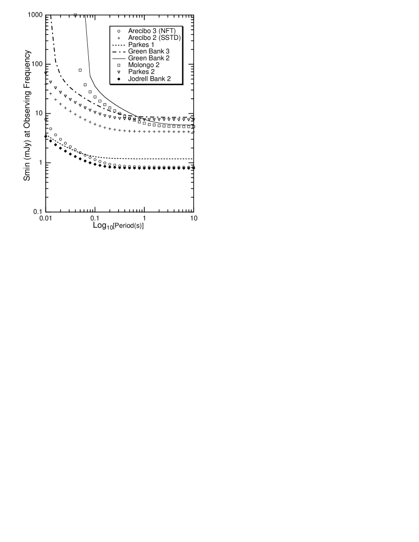
Figure 1: Radio flux thresholds, $S_{min}$, at the observing frequency for each of the eight surveys used in the simulation as a function of the pulsar period assuming a sky temperature of 150 K at 408 MHz and a dispersion measure of 200 ${\rm cm^{-3}\cdot pc}$.

These parameters are used to calculate a minimum radio flux from equation (27) that is compared to the calculated radio flux from equation (26) scaled to the observing frequency with a spectral index of $-1.7$. The efficiency of the survey (Eff. in Table 3) has been obtained from the number of survey beams times the reported solid angle at half-power beamwidth, divided by the area enclosed by the survey boundaries on the sky. The efficiency is assumed to be constant over the area surveyed. This is not the case for some of the surveys where more sampling was done in certain regions while other regions were sampled more sparely. In Figure 1, we indicate the flux thresholds for the different surveys used in the simulation assuming a sky temperature of 200 K at 408 MHz characteristic of the Galactic disk and a dispersion measure of 200 ${\rm cm^{-3}\cdot pc}$. We realize that for some surveys that do not cover this Galactic disk, this temperature might not be appropriate. We choose a common temperature for the sake of comparing the $S_{\min}$ of each of the surveys at the corresponding observing frequency. However, in the actual simulation the sky temperature at 408 MHz is obtained using the all-sky map of Haslam et al. (1982) and, then scaled to the particular observing frequency of the survey being tested. For the calculation of $S_{\min}$ in Figure 1 only, we assume a $\tau_{scat}$ obtained from the formula by Bhattacharya et al. (1992) scaled to the observing frequency and given by

$$\tau_{scat}=\left[10^{-4.62+1.14\log(DM)}+10^{-9.22+4.46\log(DM)}\right]\left({400\over{\nu}}\right)^{4.4}.$$ (32)

In the actual simulation, we obtain the scattering measure, $SM$, from the Taylor & Cordes (1993) distance model as indicated above. In Figure 1, The smallest flux thresholds occur for large periods where the intrinsic pulsar width, $W_{o}$, dominates over other terms in equation (29) resulting in a constant $S_{\min}$ from equation (27). The flux threshold increases with decreasing period when the intrinsic pulse width is dominated by the other pulse broadening terms in equation (29) and also as a result of the period dependence in equation (27). The Green Bank 2 and Molonglo 2 surveys are not very sensitive to pulsars with periods smaller than 0.1 seconds.

2.7 $\gamma$-ray Luminosity

We have taken the expressions describing the $\gamma$-ray luminosity from the work of Zhang & Harding (2000) where a polar-cap model simulates the pair cascade region, with curvature radiation of the primary particles and synchrotron radiation and inverse Compton scattering of subsequent higher generation pairs. In addition, the model uses the self-consistent acceleration model of Harding & Muslimov (1998) to produce the primary particles. The $\gamma$-ray luminosity is constrained by equation (61) of Zhang & Harding (2000) to be less than the spin-down luminosity, or

$$B_{p,12}P^{-7/4}(\cos\alpha)^{-5/4}\geq 1.65,$$ (33)

where we have used $\alpha=30^{o}$. If equation (33) is not satisfied, the $\gamma$-ray luminosity is equal to the spin-down luminosity,

$$L_{sd}=9.68\times 10^{30}B_{p,12}^{2}P^{-4}I_{45},$$ (34)

where $I_{45}$ is the moment of inertia in $10^{45}{\rm g\cdot cm^{2}}$. If equation (33) is satisfied, then the pulsar is in regime I if

$$B_{p,12}^{1/7}P^{-9/28}(\cos\alpha)^{3/28}>3.0,$$ (35)

otherwise the pulsar is in regime II. The $\gamma$-ray luminosities for the two regions are then given by the forms

$$L_{\gamma}(I)=4.8\times 10^{31}\ {\rm erg\cdot s^{-1}}\ B_{p,12}^{6/7}P^{-27/14}(\cos\alpha)^{8/7},\ {\rm and}$$

$$L_{\gamma}(II)=1.6\times 10^{31}\ {\rm erg\cdot s^{-1}}\ B_{p,12}P^{-9/4}(\cos\alpha)^{5/4}.$$ (36)

These expressions correspond to the equations (59) and (60) in the work by Zhang & Harding (2000) with an improved form for the luminosity in region I based on a more accurate expression for $E_{||}$. Equation (36) reproduces the dependence of $\gamma$-ray luminosity on $\dot{E}^{1/2}\propto B_{p}P^{-2}$ observed for CGRO detected pulsars (Thompson et al. 1997), and also agrees with the empirical luminosity law for CGRO pulsars found by McLaughlin & Cordes (2000). Having the $\gamma$-ray luminosity, we can compute the flux assuming a solid angle $\Delta\Omega$ by the form

$$S_{\gamma}={{L_{\gamma}}\over{\Delta\Omega d^{2}}},$$ (37)

where we have assumed the same solid angle of 1 steradian as in the case for the radio emission. We have used the flux thresholds (D. Thompson, priv. comm.) for in and out of the Galactic plane as indicated in Table 5.

Table 5
In and Out-of-Plane Flux Thresholds
	EGRET	GLAST
In-plane $\|b\|<10^{o}$	$1.6\times 10^{-7}\ {\rm photons/(cm^{2}\cdot s)}$	$5.0\times 10^{-9}\ {\rm photons/(cm^{2}\cdot s)}$
Out-of-plane $\|b\|\geq 10^{o}$	$7.0\times 10^{-8}\ {\rm photons/(cm^{2}\cdot s)}$	$2.0\times 10^{-9}\ {\rm photons/(cm^{2}\cdot s)}$

2.8 $\gamma$-ray Spectra

The number of simulated $\gamma$-ray pulsars depends crucially on the average $\gamma$-ray energy assumed in the calculation that converts the luminosity from erg/s to a flux $({\rm photons\cdot cm^{-2}\cdot s^{-1})}$ which gets compared to the instrument flux thresholds. If the $\gamma$-ray spectrum is assumed to be a power law of the form

$${{dN}\over{dE_{\gamma}}}=AE_{\gamma}^{-\alpha},$$ (38)

where $A$ is a normalization factor and $\alpha$ is the spectral index, the average energy above an energy threshold, $\epsilon_{th}$, can be obtained by

$$\left\langle{E_{\gamma}}\right\rangle=\left({{{\alpha-1}\over{\alpha-2}}}\right)\left({\varepsilon_{\max}\varepsilon_{th}}\right){{\varepsilon_{th}^{\alpha-2}-\varepsilon_{\max}^{\alpha-2}}\over{\varepsilon_{th}^{\alpha-1}-\varepsilon_{\max}^{\alpha-1}}},$$ (39)

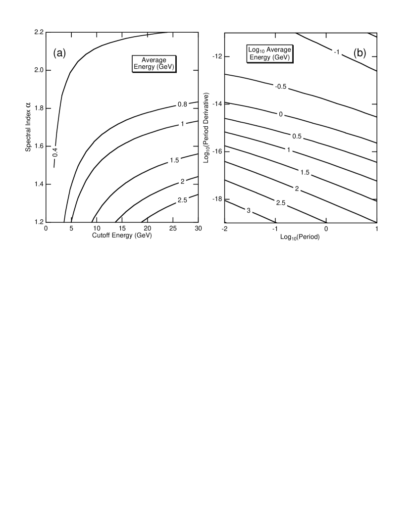
Figure 2: The average $\gamma$-ray energy (contours in GeV) from equation (39) is plotted (a) as a function of spectral index and the high energy cutoff assuming a threshold energy, $\epsilon_{th}$ = 100 MeV, typical for EGRET. bf (b) The logarithm of the average energy (contours) in GeV as a function of the logarithms of the period derivative and the period from equations (39) to (41).

where $\epsilon_{max}$ is the high energy cutoff in the spectrum. For example, typical $\gamma$-ray spectra observed by EGRET have a threshold of 100 MeV with spectral indices varying from 1.2 to 2.2 and the cutoffs vary from 5 to 30 GeV. For this range, we indicate the average $\gamma$-ray energies in Figure 2a as a function of both the spectral index and the cutoff energy.

The contours of average energies in Figure 2a reflect a flat distribution between 400 to 800 MeV where presumably most of the $\gamma$-ray pulsars exist. Rather than assuming a constant average energy for all simulated pulsars, we obtain a rough estimate of how the average energy varies with the period derivative and period of the pulsar. The spectral index of the observed $\gamma$-ray spectrum can be estimated from the polar cap cascade model (Harding & Daugherty 1999), which suggests a dependence upon the parameter $P/B_{12}$. A crude estimate of this interdependence can be represented by an expression

$$\alpha=+0.85-0.45\log\left({{P\over{B_{12}}}}\right).$$ (40)

The maximum energy in the $\gamma$-ray spectrum is attributed to the photon attenuation in the creation of electron-positron pairs as the photon propagates through the magnetosphere. The pair creation cutoff energies, $\epsilon_{max}$, can be derived from cascade codes. Baring & Harding (2000) have formulated the dependence of the maximum energies of photon escaping the magnetosphere due to pair creation at different altitudes of emission. A rough representation of these energies can be made by the following equation

$$\varepsilon_{\max}({\rm GeV})={{10}\over{B_{12}}}.$$ (41)

Having the period derivative and period dependence of the spectral index and cutoff energy from equations (40) and (41), we are able to estimate the average energies from equation (39) as a function of the period derivative and period shown in Figure 2b.

2.9 Emission Geometry

In this study, we have used a simple geometry for the radio and $\gamma$-ray emission assuming in both cases a constant emission solid angle of 1 steradian in which the radio and $\gamma$-ray beams are aligned and pointing in the direction of the Earth. There would be $4\pi$ other pulsars under the same circumstances that would not be detected because the emission cone would not be in our direction so we do not follow these in our code. Comparisons are, therefore, made between simulated radio pulsars and pulsars detected by EGRET and GLAST, observed as point sources without reference to the photon flux required for the identification of $\gamma$-ray pulsations.

2.10 Implementation

An event is initiated by selecting a neutron star with a random age, magnetic field and a fixed initial period of 30 ms. The period is evolved to the present time assuming dipole spin-down of either a constant magnetic field or an exponentially decaying magnetic field. Although the total number of neutron stars are counted, only events to the left of the multipole death line in the period derivative - period diagram are further followed. The neutron star is imparted a kick velocity due to the supernova explosion, and its trajectory is integrated from its birth location forward in time to the present. If the star is within 30 kpc of the Earth, in the viewing region of one of the surveys, and a random number is less than the geometric efficiency of the survey, the simulated pulsar is assigned a radio flux that is scaled to the observing frequency of the survey as well as a $\gamma$-ray flux above 100 MeV. We assume that the radio and $\gamma$-ray beams are aligned with an effective solid angle of 1 steradian and that the Earth is within the line of sight of the emission beams. Considering that there are a factor of $4\pi$ other pulsars whose beams are not in the direction of the Earth, we can estimate a neutron star birth rate in the Galaxy. If the scaled radio flux is above the minimum flux ($S_{\min}$) of the survey, the neutron star is flagged as a radio pulsar “observed” by that survey. Although it may be that several surveys “observed” the same pulsar, we count it as one event. Independently from the radio surveys, if the $\gamma$-ray flux is above the flux thresholds of EGRET or GLAST, it is flagged as a $\gamma$-ray pulsar observed by either EGRET or GLAST. In order to obtain smooth distributions, we continue the process until 10,000 radio pulsars are observed. As EGRET viewed (ftp://gamma.gsfc.nasa.gov/pub/PULSAR) each of the observed radio pulsars in our selected group, we normalize the distributions to the number of pulsars in the select group of observed radio pulsars. Since there are 445 observed radio pulsars in our select group that represents 90% of all the pulsars in the Princeton catalog with the features that we have specified, this normalization allows for the determination of neutron star birth rates. We compare the number of simulated $\gamma$-ray pulsars predicted to be detected by EGRET with the number that EGRET actually detected, and also predict the number of $\gamma$-ray pulsars that GLAST should be able to detect as point and as pulsed sources. In this study, we define radio-quiet $\gamma$-ray pulsars as those which are detectable by $\gamma$-ray telescopes but not by the radio surveys. In this manner, we are able to tag the events as radio-loud and radio-quiet, $\gamma$-ray pulsars “observed” by EGRET and/or GLAST. Of particular interest is the number of predicted radio-loud and radio quiet, $\gamma$-ray pulsars, how they compare to those observed by EGRET as point sources and where each of these source groups are located in the $\dot{P}-P$ diagram.

3 Results

For the purpose of this study, we have focused on performing simulations for two different cases: one in which the magnetic field remains constant and a pulsar death valley in the period derivative-period diagram is assumed and one in which the magnetic field is allowed to decay exponentially without a death valley. We have placed greater emphasis on the case where the field is constant.

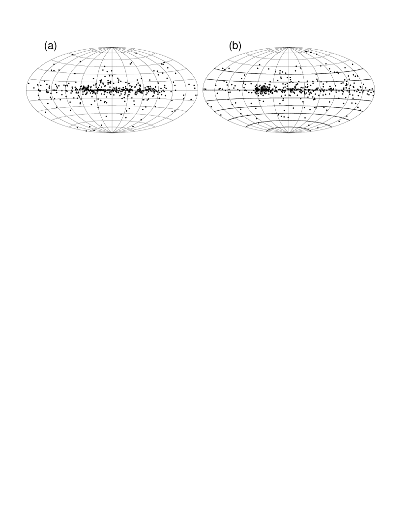
Figure 3: Aitoff plots of the observed pulsars (a) and of the simulated pulsars (b) for the case of no field decay and a death valley.

In Figure 3, we present a comparison of the observed (3a) and simulated (3b) distributions of 445 pulsars shown in Galactic coordinates as Aitoff projections. The simulation assumes no field decay. The distributions are governed in part by the survey regions that have been chosen, but also by the many primary distributions such as birth location and Galactic potentials, etc. As can be seen, the calculated and observed distributions are very similar. In this preliminary study, we do not expect to reproduce the exact numbers observed by each survey. The number of pulsars observed depends crucially on the assumptions made in the determination of $S_{\min}$ and the geometric observing efficiency. As mentioned, we have neglected the last time-smearing term in equation (29), we have assumed a constant duty fraction of 0.05 for the intrinsic pulse width for all periods and all surveys, we have assumed a constant receiver temperature, and we have assumed that the efficiency is constant over sky boundaries of the surveys. We hope to improve these assumptions in a subsequent study that includes a realistic representation of the emission geometries for both the radio and $\gamma$-ray beams. Yet we affirm that this preliminary investigation makes important contributions to the understanding of pulsar emission and paves the way for further studies.

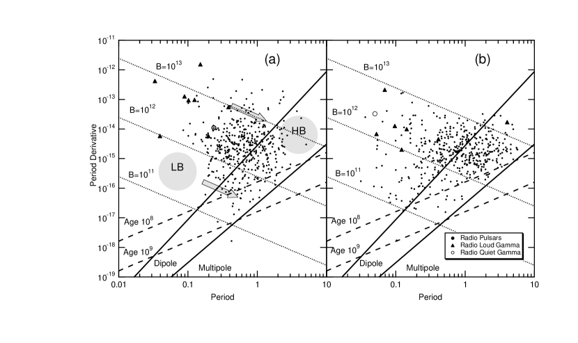
Figure 4: Distributions of observed pulsars (a) and simulated pulsars (b) for the case of no field decay and a death valley as a function of the period derivative and period (in seconds) of the pulsars. Solid dots indicate radio pulsars. Solid triangles represent radio-loud, $\gamma$-ray pulsars and open circles symbolize radio-quiet, $\gamma$-ray pulsars observed (a) and predicted (b) for EGRET.

In Figure 4, we compare the period-derivative versus period $(\dot{P}-P)$ plot of the select group of observed pulsars (4a) with the one of simulated pulsars (4b). The dotted lines are shown for the locus of constant magnetic field with the indicated strength. The dashed lines represent the indicated ages of pulsars assuming a dipole spin-down field. The solid lines show the pulsar death lines for dipole and multipole magnetic field distributions in the curvature-initiated, space-charge-limited-flow model (SCLF) (Zhang, Harding & Muslimov 2000). The radio pulsars observed (4a) and those simulated and filtered (4b) through the select group of surveys are indicated with solid dots.

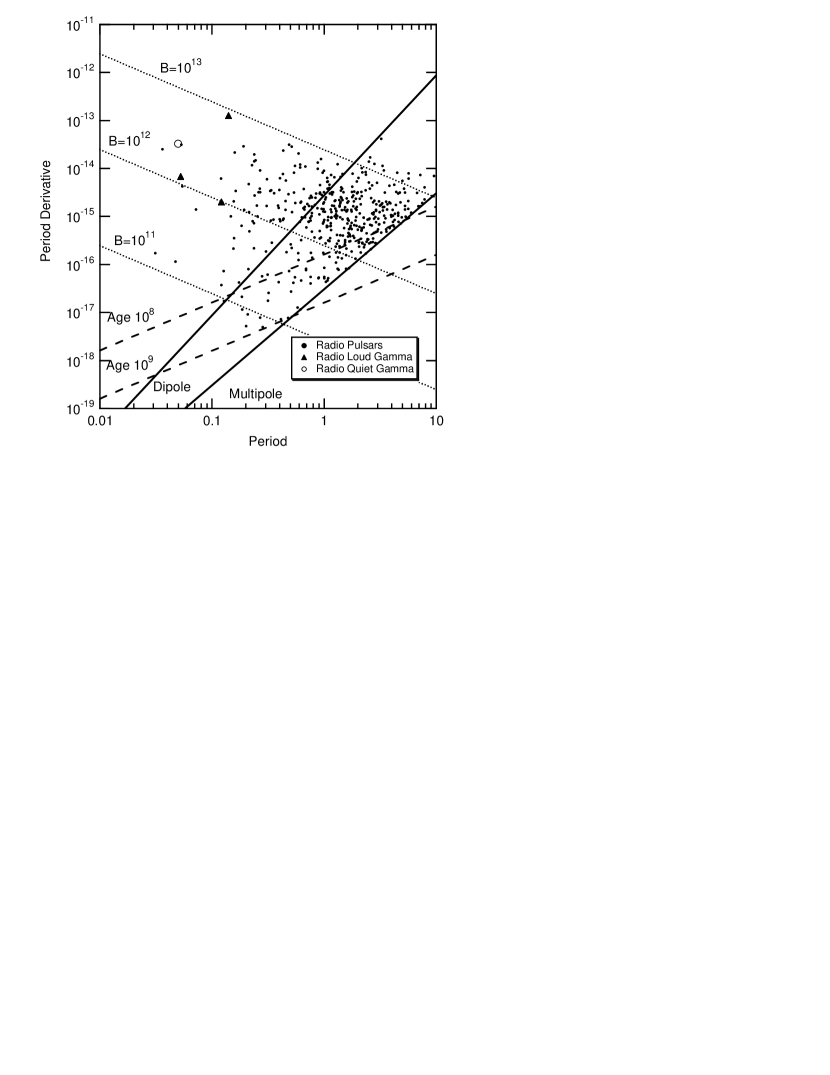
Figure 5: Distributions of simulated pulsars as a function of the period derivative and period for case of no field decay and no death valley. Solid dots indicate radio pulsars. Solid triangles represent radio-loud, $\gamma$-ray pulsars and open circles symbolize radio-quiet, $\gamma$-ray pulsars predicted for EGRET.

Radio-loud and radio-quiet, $\gamma$-ray pulsars are represented with solid triangles and open circles, respectively. The observed radio-quiet, $\gamma$-ray pulsar is Geminga and a list of radio-loud, $\gamma$-ray pulsars detected by EGRET includes Vela, the Crab, B1951+32, B1706-44, B1509-58, B1055-52, B0656+14 and J1048-5832. The pulsar J0218+4232 with a period of 2.32 ms and a period derivative of $7.5\times 10^{-20}\ {\rm s\cdot s^{-1}}$ is outside the bounds of the plot and of the characteristics of the select group of pulsars. The simulations for this case result in 7 radio-loud and 1 radio-quiet, $\gamma$-ray pulsars “observed” by EGRET (shown in Figure 4b) and 76 radio-loud and 74 radio-quiet, $\gamma$-ray pulsars “observed” by GLAST. The previously mentioned death valley operates between these two lines where the code exponentially ($\propto e^{(-d/\tau)}$) removes excess pulsars with a decay constant of $\tau=1.0$ in a random fashion depending on the pulsar’s distance, $d$, from the multipole death line along a constant magnetic field. Figure 5 shows the simulated distribution using the same set of parameters as those that generated Figure 4b except without the death valley in effect.

Clearly the excess of pulsars near the multipole death line in Figure 5 is not seen in the observed distribution in Figure 4a. However, there are still significant differences even with the presence of the death valley in comparing Figures 4a and 4b. The observed distribution of radio pulsars is narrower in period, elongated up and down along the period derivative axis, whereas the simulated distribution is elongated left and right along the period axis. The observed distribution has more pulsars with smaller period derivatives and fewer high field pulsars in the death valley than simulated distribution. The observed distribution of low field pulsars is narrower in period than that simulated, while the distribution of high field pulsars is broader than that simulated. Broadening the primary high field Gaussian (Table 1) or including a higher field component only increases the number of high field pulsars bunched up near the multipole death line and cannot reproduce the group of high field pulsars observed with periods between 0.1 and 2 seconds in Figure 4a.

The observed group of $\gamma$-ray pulsars is on average younger, with larger $\dot{P}$ and higher fields, than the group of simulated pulsars. However, the one observed radio-quiet, $\gamma$-ray pulsar is older with a higher field than the 1 predicted. An important factor in the selection of the $\gamma$-ray pulsars is the assumed flux thresholds (Table 5). The comparison of the observed and simulated distributions in Figure 4 suggests that there are fewer observed pulsars with higher periods than in the simulated distribution. It might be that in addition to the minimum radio flux dependence on the period described in equation (27) there is a high period limit to the radio surveys where typically the radio sensitivity increases with increasing period. However, there is in some published figures a slight increase in $S_{min}$ for pulsars with periods greater than a few seconds (Dewey et al. 1985 and Stokes et al. 1986), perhaps due to computations of the actual telescope $S_{min}$ during the observing period. As there are no details given in these publications, we have not taken this into account in our model simulations.

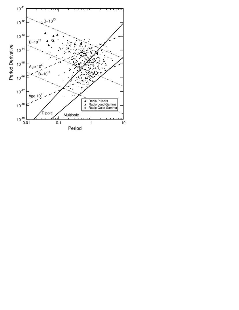
Figure 6: Distributions of simulated pulsars as a function of the period derivative and period of simulated pulsars for case of magnetic field decay, assuming a time constant of $5\times 10^{6}$ years, and no pulsar death valley. Solid dots indicate radio pulsars. Solid triangles represent radio-loud, $\gamma$-ray pulsars and open circles symbolize radio-quiet, $\gamma$-ray pulsars predicted for EGRET.

The clear absence of high-field, high-period observed pulsars in Figure 4a indicated by the shaded circle labeled HB (High field) as compared to those simulated in Figure 4b, might be suggestive of the decay of the magnetic field. There are observed pulsars in the region indicated by the arrow that should have led to pulsars in the HB region. In fact, the whole wedge-shaped distribution of observed pulsars in Figure 4a could be explained by field decay, including the absence of low-field observed pulsars in the shaded region labeled LB (low field). If the field does not decay, one would expect pulsars in this region (LB) to have led to the observed low-field pulsars indicated by the arrow. The excess of simulated high-field, high-period pulsars have ages of the order of $10^{7}$ years. Therefore, a decay constant of this order is required for these high-field pulsars to have their fields decay by an order of magnitude. In Figure 6, we present a simulation in which we have included the decay of the magnetic field with a time constant equal to $5\times 10^{6}$ years. In this simulation, we removed the death valley to facilitate comparison with Figure 5 where we have simulated pulsars without the pulsar death valley to directly see the effects of the field decay. With field decay, the pulsars do not seem to bunch-up along the multipole death line as in Figure 5 as the field decreases with age, producing a wedge-shaped distribution at low fields, small period derivatives and mid-periods.

We found that the multiple low-field and high-field Gaussians used in the main simulations (see Table 1) were not necessary to achieve a distribution comparable to the observed distribution in Figure 4a. The improvement is quite noticeable. The wedge-shaped distribution of the observed pulsar distribution is explained, even in the region of low period and moderate period derivative, where the simulation in Figure 4b has an over abundance of pulsars (LB) in comparison to the observed distribution. The simulations for this case result in 9 radio-loud and 2 radio-quiet, $\gamma$-ray pulsars “observed” by EGRET (shown in Figure 6) and 90 radio-loud and 101 radio-quiet, $\gamma$-ray pulsars “observed” by GLAST. Introducing the pulsar death valley along with the field decay would remove pulsars from the death valley and yield more pulsars to the left of the valley, thereby, increasing the number of radio-loud, $\gamma$-ray pulsars. The simulation with field decay suggests that the death valley might not be a required artifact to have reasonable agreement with the number of radio-loud, and radio-quiet, $\gamma$-ray pulsars detected by EGRET. The main difficulty in accounting for the observed shape of the pulsar distribution by field decay is being able to justify the small time constant of $5\times 10^{6}$ years. Several mechanisms for field decay in neutron stars have been studied (e.g. Goldreich & Reisenegger 1992). Ohmic diffusion, with a decay timescale $\sim 2\times 10^{11}{\rm\ yr}\,L_{5}^{2}/T_{8}^{2}$, where $L_{5}$ is the characteristic length scale of the flux loops in units of $10^{5}$ cm and $T_{8}$ is the core temperature in units of $10^{8}$ K, dominates in fields $B<10^{11}$ G. Hall drift in the crust, with a timescale $\sim 5\times 10^{8}{\rm\ yr}\,L_{5}^{2}T_{8}^{2}/B_{12}$, dominates in fields $B\sim 10^{12}-10^{13}$ G. Ambipolar diffusion, with a decay timescale $\sim 3\times 10^{9}{\rm\ yr}\,L_{5}^{2}T_{8}^{2}/B_{12}^{2}$, dominates at the highest fields. Thus, for fields $B\sim 10^{9}-10^{13}$ characteristic of the radio pulsar population, the decay timescale is longer than $3\times 10^{7}$ yr. However, if the birth distribution of fields has a mean of around $2\times 10^{13}$ G, then the average initial decay timescale would be $\sim 5\times 10^{6}$ yr. But since the decay timescale is a strong function of field strength, this initially short decay timescale would not persist as the field decreases. Clearly, a more detailed study is required to fully address the effect of realistic field decay in the radio pulsar population studies.

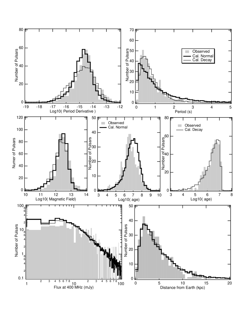
Figure 7: Distributions of various pulsar characteristics indicated as shaded histograms (observed pulsars) and plain histograms (simulated pulsars). Thick histograms represent the distributions of the simulated pulsars assuming no field decay and pulsar death valley, while the thin histograms result from the case assuming field decay and no death valley.

In Figure 7, we compare various distributions of the indicated features of observed pulsars (shaded) and of simulated pulsars. The smooth simulated histograms have been obtained from a group of 10,000 pulsars and then normalized to a total of 445 pulsars, the number of the selected group of observed pulsars. The dark histograms represent the case in which there is no field decay and a pulsar death valley is assumed as discussed previously. The light histograms result from the simulation of the field decay case with no death valley. Under the assumption of field decay, the pulsar age depends on the decay constant of the magnetic field (5 Myr). As a result, we show separate figures for the pulsar age distributions. As noted for the case of no field decay, too many older pulsars with long periods and with small period derivatives are produced in our simulation. However, the simulated distributions of radio flux and distance from Earth along with the magnetic field agree very well with those observed. The distributions for the case of field decay overall appear to better describe the observed distributions without the necessity of introducing a pulsar death valley between the dipole and multipole death lines.

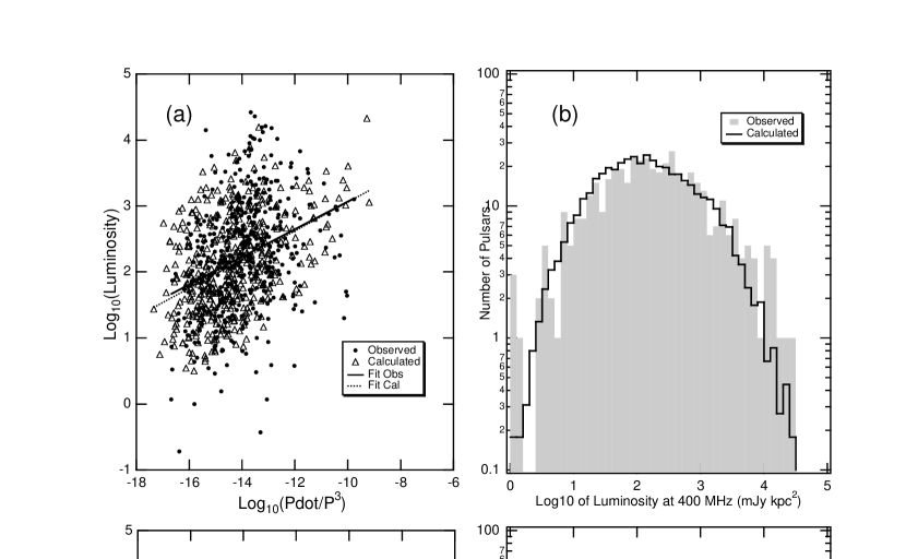
Figure 8: The logarithm of the radio luminosity as a function of the $\log(\dot{P}/P^{3})$ for the cases of an intercept of 7.2 (a) and 6.64 (c). Pulsars are simulated assuming no magnetic field decay and the presence of a death valley between the death lines. Observed and simulated pulsars represented by solid dots and open triangles, respectively. Linear fits of the observed and simulated distributions are represented by solid and dotted lines, respectively. The distributions of the logarithm of the radio luminosity at 400 MHz for observed (shaded histogram) and predicted (plain histograms) pulsars for the cases of an intercept of 7.2 (b) and 6.64 (d). We find that similar results are obtained assuming field decay.

The period and period derivative dependence of the radio luminosity is another important function that crucially determines the radio selection of simulated pulsars. As mentioned previously, we have used the functional form developed by Bhattachary et al. (1992) who followed the work of Narayan & Ostriker (1990), Vivekanand & Narayan (1981) and Prószyński & Przybycién (1984) and found the best fit for a luminosity function described by equation (25). While we do not wish to develop a fitting model in this study, we found that it was necessary to slightly adjust the intercept of their functional form from 6.64 to 7.2. We present in Figure 8 a comparison of the radio luminosity distribution at 400 MHz $(\log_{10}\langle L_{400}\rangle)$ as a function of $\log_{10}(\dot{P}/P^{3})$ and the population distributions of the radio luminosity for observed and simulated pulsars displayed as histograms. In the $\log_{10}(L_{400})$ versus $\log_{10}(\dot{P}/P^{3})$ plots, we performed linear fits in order to make comparisons of the distributions. The resulting fit parameters are indicated in Table 6.

Table 6
Linear Fit Parameters
	Intercept	Slope
Observed	$5.2\pm 0.4$	$0.21\pm 0.03$
6.64 intercept in Eqn. 22	$5.0\pm 0.3$	$0.23\pm 0.02$
7.2 intercept in Eqn. 22	$5.2\pm 0.3$	$0.21\pm 0.02$

Note that we do not expect to obtain the same parameters as in equation (25), which represents the average radio luminosity of the primary pulsars prior to being observed. The modified luminosity law with an intercept of 7.2 also fits well the luminosity distributions for the case assuming the decay of the magnetic field. The actual radio luminosity at 400 MHz is dithered about the average using the function described in equation (23) and (24). Hartman et al. (1997) describe how the parameters of the dithering function affect the net luminosity distribution. The work of Narayan & Ostriker (1990) was done with a sample of 265 pulsars known at the time with measured period and period derivative obtaining a functional form that has been used quite often in the literature. However, it seems clear that with a much larger sample of pulsars, a better functional form needs to be obtained. This functional form of the radio luminosity plays an important role in the selection of a radio pulsar and in the ratio of radio-quiet to radio-loud, $\gamma$-ray pulsars. Clearly the required dithering about the average luminosity masks some dependence that is currently not understood, perhaps reflecting some dependence of the emission geometry on the period as suggested by Kijak & Gil (1998) and Rankin (1993).

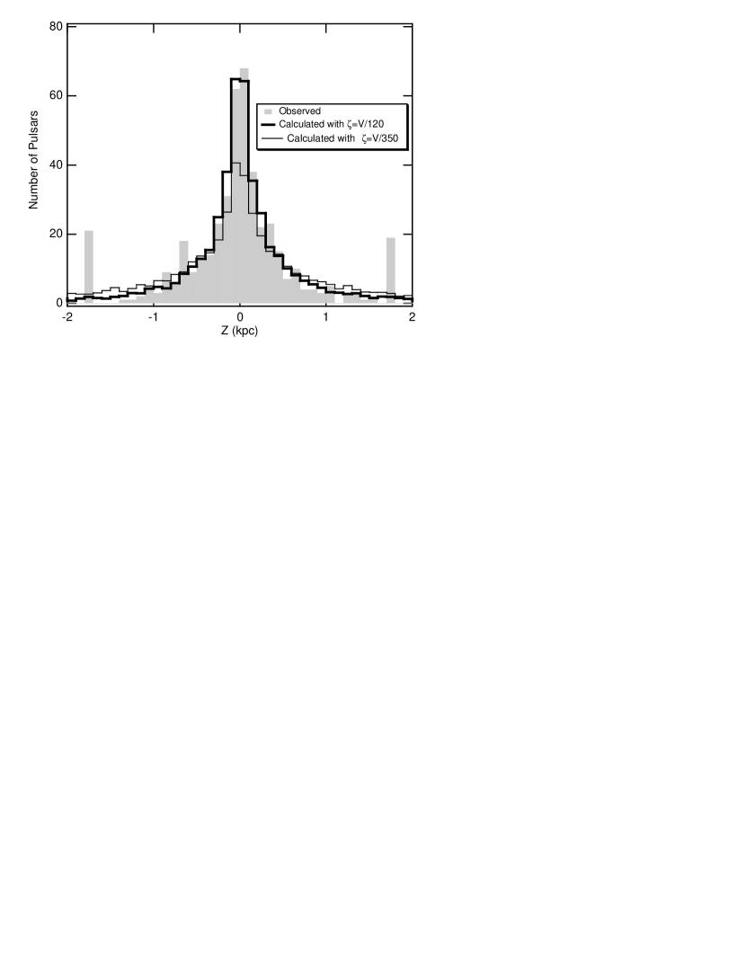
Figure 9: The $z$ distribution from the Galactic disk for observed (shaded histograms) and simulated pulsars for the cases of $\zeta=v/120$ (thick line) and of $\zeta=v/350$ (thin line) assuming no field decay and a death valley. For the case of field decay, the simulated distribution is slighty narrower with a width of $0.14\pm 0.01\ kpc$.

Another important parameterization of the primary pulsars is the initial velocity kicks given to pulsars at the time of their birth from asymmetric supernova explosions. These velocity distributions have been discussed extensively by Dewey & Cordes (1987), Lyne & Lorimer (1994), Bailes (1989), van den Heuvel & van Paradijs (1997), and Lorimer, Bailes & Harrison (1997) indicating space birth velocities of 400 - 500 km/s. Hansen & Phinney (1997) indicate that these studies did not include the selection effects from flux limits of the pulsar surveys or the accuracy of the proper motion determinations and conclude that a Maxwellian distribution with a mean velocity of 300 km/s adequately describes the observations. More recently, a study undertaken by Cordes & Chernoff (1998) concludes that the three-dimensional velocity distributions can be best accounted for using a two component Gaussian function with mean velocities of 175 and 700 km/s representing 86 % and 14 % of the population. In this study, we have chosen to use the functional form of Lyne & Lorimer (1994) with some modification. We used the $z$ distribution of the radio pulsars from the Galactic disk to establish the kick velocity parameter. In Figure 9, we present the $z$ distribution (shaded) of observed pulsars from our select group of 445.

The spikes at $\approx 1.7$ kpc reflect the limitation of the distance model (Taylor & Cordes 1993). The thin and thick solid histograms represent the simulated distributions using $\zeta=v/120$ km/s used in this study and $\zeta=v/350$ km/s used by Lyne & Lorimer (1994), respectively. Since the primary $z$ distribution of pulsars is assumed to be exponential, we have fit the observed and simulated distributions shown in Figure 9 with exponential forms obtaining the following widths shown in Table 7.

Table 7
Widths (kpc) of Exponential Fits of the z Distribution
Observed	For $\zeta=v/120\ {\rm km/s}$	For $\zeta=v/350\ {\rm km/s}$
$0.18\pm 0.01$	$0.18\pm 0.01$	$0.34\pm 0.01$

The functional form of Lyne & Lorimer with a parameter of $\zeta=v/350$ km/s results in a distribution with most probable and average velocities of 266 and 494 km/s, respectively, and leads to a significantly broader distribution twice the width of the observed distribution. Much better agreement is obtained with a parameter of $\zeta=v/120$ km/s with a most probable and average velocities of 91 and $168$ km/s, respectively. We do find that the $z$ distribution is slightly sensitive to other parameters of our model described in this study. Again we are trying to use the best available distributions of pulsar features, but comparing the resulting distributions “by eye” has required us to make some small changes. The agreement is equally good for the case assuming the decay of the magnetic field with a slight narrower distribution with a width of $0.14\pm 0.01\ kpc$. As a result, we have used this same velocity distribution for both the cases where the field is constant and is allowed to decay.

In Figure 10, we present a set of $\dot{P}-P$ diagrams for radio-quiet, $\gamma$-ray pulsars as seen by EGRET (10a) and GLAST (10b) and for radio loud, $\gamma$-ray pulsars as seen by EGRET (10c) and GLAST (10d) represented by solid circles. We have also included the group of $\gamma$-ray pulsars detected by EGRET in Figures 10a and 10c shown by solid triangles. In order to obtain smoother distributions of these different groups in the $\dot{P}P$ diagram, we have simulated a group of 10,000 pulsars and depict their distributions by the contoured regions. The gray scaled background represents the energy-integrated $\gamma$-ray and average radio luminosities in the upper panels (10a and 10b) and in the lower panels (10c and 10d), respectively. The average radio luminosity is proportional to $\dot{P}^{1/3}P^{-1}$, while the $\gamma$-ray luminosity in regime II drops faster and is proportional to $\dot{P}^{1/2}P^{-7/4}$. The most intense luminosities for both radio and $\gamma$ rays are in the upper left in the $\dot{P}-P$ diagram, but here the pulsars are very young and few in number. The numbers indicated in the legend represent the number of simulated pulsars from the group of 445 radio pulsars. The model predicts that GLAST should observe 76 radio-loud, $\gamma$-ray pulsars compared to 7 predicted for EGRET detected as point sources. The model predicts that GLAST should observe 74 radio-quiet, $\gamma$-ray pulsars compared to 1 predicted for EGRET. The GLAST sensitivity for blind period searches is expected to be about the same as the EGRET point-source detection sensitivity (S. Ritz, priv. comm.). GLAST will, therefore, be expected to identify 7 of these 74 objects as pulsed sources. The distribution of radio-loud, $\gamma$-ray pulsars predicted to be observed by GLAST peaks at a lower $\gamma$-ray luminosity towards the more populated region of radio pulsars than the distribution predicted for EGRET. Due to the greater sensitivity of GLAST, the group of radio quiet, $\gamma$-ray pulsars also moves toward lower $\gamma$-ray luminosities and more populated regions in the $\dot{P}-P$ space, but the radio-quiet pulsars are younger.

The radio-quiet pulsar, Geminga, observed by EGRET is located in the GLAST region of radio-quiet pulsars in Fig. 10, but somewhat removed from the EGRET region. The results of the simulation seem to agree fairly well with the observations made by EGRET though, perhaps, predicting a few too many radio-loud, $\gamma$-ray pulsars. As mentioned before, many of the EGRET unidentified sources are expected to be radio-quiet, $\gamma$-ray pulsars.

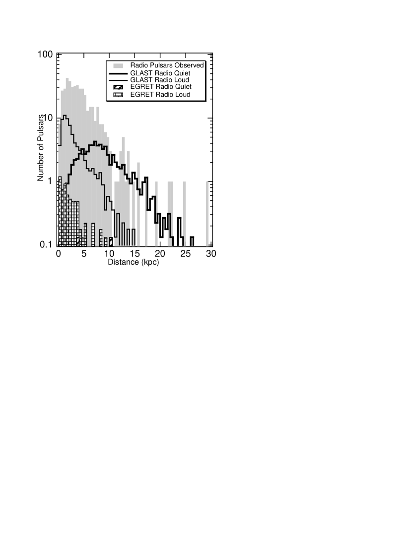
Figure 11: Distributions of the distance from Earth of observed radio pulsars (shaded histograms), radio-loud (thick histograms) and radio-quiet (thin histograms), gamma pulsars for GLAST), radio-loud (brick patterned histograms) and radio-quiet (diagonally patterned histograms), gamma pulsars for EGRET. The simulated distributions are for the case of no magnetic field decay and the presence of a pulsar death valley.

The results predicted for GLAST are interesting in that about as many radio-quiet, $\gamma$-ray pulsars are expected to be observed as radio-loud, $\gamma$-ray pulsars. Given the flux thresholds we have used, these are objects observed as point sources. In order to understand why GLAST is predicted to detect a larger ratio of radio-quiet to radio-loud, $\gamma$-ray pulsars than EGRET, we present in Figure 11 the distribution of the distance of the pulsar from Earth for each of these groups. We simulated a group of 10,000 radio pulsars and normalized the distributions to the number (445) of observed radio pulsars in the selected group. As a result, one can see fractional numbers of pulsars in the distributions. The distribution of observed radio pulsars is presented as a shaded histogram. The predicted distributions of radio-quiet (thin) and radio-loud (thick), $\gamma$-ray pulsars for GLAST are displayed by the plain histograms. The predicted distributions of radio-quiet (diagonal pattern) and radio-loud (brick pattern), $\gamma$-ray pulsars are indicated for EGRET. The distribution of radio-loud, $\gamma$-ray pulsars detected by both EGRET and GLAST have distributions with similar shapes as the observed radio distribution. Due to significantly different $\gamma$-ray flux thresholds, the distributions of radio-quiet, $\gamma$-ray pulsars are quite different for EGRET and GLAST. Thus the simulation suggests that due to the increased sensitivity, GLAST will be able to detect more pulsars that are further away than even those detected by the radio surveys used in this study. This may change with the observations from the Parkes multibeam pulsar survey (Manchester et al. 2001) that has been finding more young, distant pulsars.

In Table 8, we summarize the number of radio-quiet and radio-loud, $\gamma$-ray pulsars simulated for the two main cases explored in this study in which we have assumed no magnetic field decay requiring a pulsar death valley and field decay without a death valley. The results for the case of no field decay without a valley are also included for comparison. In addition, we have indicated the number of pulsed sources that GLAST would observe from the radio-quiet, $\gamma$-ray pulsar group.

Table 8
Simulated Pulsar Statistics
	EGRET		GLAST		Neutron Star Birth
Case	Radio Quiet	Radio Loud	Radio Quiet (Pulsed)	Radio Loud	Rate (per century)
No decay
with valley	1	7	74 (7)	76	1
No decay
no valley	1	3	35 (3)	38	0.5
Decay
no valley	2	9	101 (9)	90	2

These simulations are able to suggest a neutron star birth rate. As mentioned previously, we have assumed a 1 steradian solid angle of the radio beam, so there is a factor $4\pi$ more pulsars whose beams do not point in the direction of the Earth than those used in the simulation. We indicate in the table the estimated neutron star birth rates per century for each of the indicated cases. We have corrected the birth rates assuming a Gaussian beam to correct the overall detection by the ratio of the detection volume to that of the actual volume that increases the birth rate by a factor of 1.4 (Arzoumanian, Chernoff & Cordes 2001).

4 Discussion

We have modeled the Galactic population of radio pulsars using a Monte Carlo simulation in order to calculate the expected numbers of $\gamma$-ray pulsars detectable by EGRET and GLAST. This paper has focused on the $\gamma$-ray luminosity predicted by the polar cap model of Daugherty & Harding (1996) and Zhang & Harding (2000). Our simulation predicts about the same number of radio-loud $\gamma$-ray pulsars (7) compared to the number (8) detected by EGRET. We predict that GLAST should detect on the order of bf 75-100 radio-loud pulsars, however this number could also change with a detailed treatment of geometry. A very interesting, and somewhat unexpected, result of our simulation is the prediction that GLAST will detect about the same number (74) of radio-quiet as radio-loud pulsars (76), at least as point sources. Since we have assumed that the radio and $\gamma$-ray beams are identical in this study, this result implies that GLAST will be more sensitive than radio surveys with regard to the detection of young pulsars in the Galaxy. Even with the considerable model uncertainties, we can conclude that polar cap models predict a much smaller ratio of radio-quiet to radio-loud $\gamma$-ray pulsars than do outer gap model studies. For example, Zhang, Zhang & Cheng (2000) predict that GLAST will detect only about 80 radio-loud $\gamma$-ray pulsars but about 1100 radio-quiet $\gamma$-ray pulsars. This ratio then, regardless of the exact numbers, will be an important discriminator between polar cap and outer gap models.

We have found that magnetic field decay could have a significant effect on pulsar evolution and the formation of the observed pulsar $\dot{P}-P$ distribution. As mentioned previously, there are distinct differences between the observed distribution of Figure 4a and the simulation without field decay of Figure 4b. There is an over abundance of simulated pulsars with high fields and high periods. The apparent drop in observed pulsars in this region could be conceived as evidence for the decay of the magnetic field. Our preliminary calculations suggest that a decay constant of the order of $10^{7}$ years is required to effect such a distribution, as also suggested by the ages of these pulsars in this region. A recent study of the radio pulsar distribution by Tauris & Konar (2001) also concludes that some torque decay is required. Most studies of field decay estimate longer decay constants in fields below $B\sim 10^{13}$ G. However, we believe that this issue warrants further study.

We can analytically calculate the time it takes a pulsar from birth with a given magnetic field to reach the multipole death line. Since we are assuming a constant birth rate, dividing this time by the maximum age of $10^{9}$ years used in the simulation provides a survival fraction of initial pulsars found to the left of the multipole line and is given by the expression

$$F_{s}=9.0\times 10^{-3}B_{12}^{-6/7}.$$ (42)

From this equation, one can see that as the magnetic field increases by an order of magnitude, the survival fraction will decrease by an order of magnitude. This explains why the factor $A_{3}$ in Table 1, though much smaller than $A_{1}$, makes a significant contribution. The initial population is weighted by this primary distribution of the magnetic field. Looking at the wings of the field distribution say at $10^{13}$ G and $10^{11}$ G, assuming no selection effects, these pulsars would be randomly distributed over time with 90% of them lying between the age lines of $10^{8}$ and $10^{9}$ years. However, the radio luminosity, being proportional to $\dot{P}^{1/3}P^{-1}$, is dropping toward the multipole line. Therefore, pulsars with shorter periods to the left of the multipole line are more radio luminous and are seen scattered to the left of the line for an age of $10^{8}$ years. The simulation indicates a broader distribution in period along the $B=10^{11}$ G line than the distribution along the $B=10^{13}$ G line. The observed distribution shows the opposite effect in these regions with a narrower distribution along the $B=10^{11}$ G line with very few pulsars with periods less than 0.2 seconds and a broader distribution along the line $B=10^{13}$ G that cuts off the number of pulsars dramatically beyond a 2 second period. The paucity of pulsars at low periods is maybe related to several effects that we have not accounted for in this simulation. Perhaps we have underestimated the actual minimum radio flux threshold given theoretically by equation (27) and plotted in Figure 1. The flux threshold tends to increase dramatically for some surveys for periods less than 0.1 s (as in the cases the Molonglo 2 and Green Bank 2 surveys with rather large sampling rates), which is where the observed distribution in Figure 4a begins to indicate fewer pulsars than the simulated distribution in Figure 4b. This may be a result of the fact that we have left out the fifth term in equation (29), which becomes significant for low period pulsars and is more significant for the Green Bank 3 and Arecibo 2 surveys. We hope to add this term to our next simulations when we also take into account the emission geometry. However, this is not a problem for the newer surveys with smaller sampling rates. With the exception of the Jodrell Bank 2 and Parkes 1 survey, the surveys were performed at low frequencies around 420 MHz. Young pulsars with short periods and large period derivatives are distant and in the Galactic plane where the effects of scattering and background temperatures require a more careful treatment than we have done in this simulation.

On the other hand, the group of high field, large period pulsars missing in the observed distribution may be a manifestation of the effects of the geometry of the radio beam. Various studies (Arzoumanian, Chernoff & Cordes 2001, Kijak & Gil 1998, Gil & Han 1996 and Rankin 1993) suggest that the pulse width of both the core and conal emission beams is proportional to $P^{-1/2}$. Therefore, as the period increases, the solid angle of the emission decreases. The observed distribution in Figure 4a seems to indicate a decrease of pulsars above a period of about 2 seconds across magnetic field strengths higher than $10^{12}$ G to the left of the multipole death line, which is also reflected in Figure 7 where the simulation predicts too many older pulsars. We expect that our forthcoming model with more realistic geometries will yield better agreement in this region.

In our model, we introduced a death valley to drastically reduce the number of pulsars between the dipole death lines and the multipole death line. As the pulsars age along constant field lines between these lines both the $\gamma$-ray and radio luminosities are decreasing as well as the spin-down energy. Cascade simulations (Baring & Harding 2001) suggest that the density of electron-positron pairs is also decreasing in a similar fashion. While there has been no firm theoretical development to connect the pair density and the radio luminosity, one can speculate that there must be a definite relationship, and the radio luminosity must decrease in some manner with decreasing pair density. Perhaps the need for the death valley also reflects the geometric relationship of the radio beam to the period, as discussed above.

There is also an interdependence of the derived velocity distribution, radio luminosity function and field evolution. For example, the velocity distribution predicted by Lyne & Lorimer (1994) does not fit the observed z distribution assuming the luminosity model of Narayan & Ostriker (1990). Using their distribution, we find a width of the z distribution that is twice that of the observed distribution as shown in Figure 9. Our simulations suggest that most of the pulsars can be accounted for with a smaller mean velocity of 170 km/s, which we found to be essentially independent on whether the field decays or not. Clearly there are pulsars with space velocities of at least one thousand km/s. However, we did not attempt to introduce a second distribution of high velocities as in the case of the study by Cordes & Chernoff (1998) and Arzoumanian, Chernoff & Cordes (2001). We have also been careful to check that the distance distribution of the simulated pulsars agrees with the observed distribution as noted in Figure 7. If the pulsars are too radio bright, more pulsars further away will be detected in the simulation causing the distribution to shift further away. Assuming the distance model is correct, we adjusted the Narayan & Ostriker (1990) luminosity law based on the observed luminosity distributions shown in Figure 8. The luminosity model of Narayan & Ostriker (1990) is also somewhat dependent on their assumption of field decay, for which they studied several cases with decay constants ranging from 8 million to 11 million years. Bhattacharya et al. (1992), using the same luminosity model, found similar results for decay constants of 10 and 100 million years, although the study of Hartman et al. (1997), which did not include magnetic field decay, also used this same luminosity law. So the luminosity model, velocity distribution and field evolution remain uncertain, especially without the inclusion of the geometry of the radio beams.

A population of radio-quiet, $\gamma$-ray pulsars results very naturally from the different dependence upon the pulsar period and period derivative of the radio and $\gamma$-ray luminosities. With the same beam geometry for both radio and $\gamma$-ray emission, the model predicts a few radio-quiet, $\gamma$-ray pulsars, like Geminga, that EGRET should have observed as well as about the right number of radio-loud, $\gamma$-ray pulsars. The number if radio-quiet $\gamma$-ray pulsars is likely to increase with a more realistic treatment of beaming geometry. Within the EGRET Third Catalog, there are 171 unidentified $\gamma$-ray point sources, many of which could be radio-quiet, $\gamma$-ray pulsars, an issue that will be settled by GLAST with its ability to perform period searches.

If there were no selection effects imposed, the main concentration of pulsars would be near the multipole death line. Since the average radio luminosity is proportional to $\dot{P}^{1/3}P^{-1}$, the observed radio population is pushed away from the multipole death line towards the upper left portion of the $\dot{P}-P$ diagram. The average $\gamma$-ray luminosity is proportional to $\dot{P}^{1/2}P^{-7/4}$ and, therefore, drops faster than the radio luminosity pushing the population of $\gamma$-ray pulsars even higher toward the upper left, especially in the case of EGRET with higher thresholds than GLAST as seen in Figure 10. With greater sensitivities of GLAST, the $\gamma$-ray pulsar population moves more to the lower right to correspond more with the region of the population of radio pulsars as also noted in Figure 10d. However, with the lower $\gamma$-ray flux thresholds expected for GLAST, it will be able to observe more pulsars at larger distances than those observed by the radio telescopes that were used in the observations of the select group of pulsars in the catalog. As a result, the expected number of radio-quiet, $\gamma$-ray pulsars increases relative to the radio-loud, $\gamma$-ray pulsars from those observed by EGRET.

The ratio of radio-quiet to radio-loud, $\gamma$-ray pulsars is strongly sensitive to the assumptions for the geometries of the radio and $\gamma$-ray beams. In this study, we assumed a simple geometry that accords with the polar cap model where the region of radio and $\gamma$-ray emission are tied to the magnetic polar cap area and are very similar. The outer gap model, on the other hand, suggests a very different geometry for the $\gamma$-ray beam, which originates on field lines of the opposite pole from that of the visible radio beam. These outer gap models (Romani & Yadigaroglu 1995, Cheng & Zhang 1998, Zhang, Zhang & Cheng 2000) predict that GLAST will detect many more radio-quiet, $\gamma$-ray pulsars. In a model independent study, MacLaughlin & Cordes (2001) simply assume a large solid angle ($2\pi$) for the $\gamma$-ray beam and predict that GLAST will detect around 120 radio-loud and 750 radio-quiet pulsars. Polar cap models predict that older pulsars with ages greater than $10^{6}$ years and with longer periods should emit $\gamma$ rays, while the outer gap models predict that such pulsars will be radio-quiet (Chen & Ruderman 1993). bf While the simple model studied here provides strong diagnostics, in the near future, we hope to perform simulations with a model that includes a more realistic geometry for the radio as well as the $\gamma$-ray beams and should provide further understanding that may help differentiate between pulsar models.

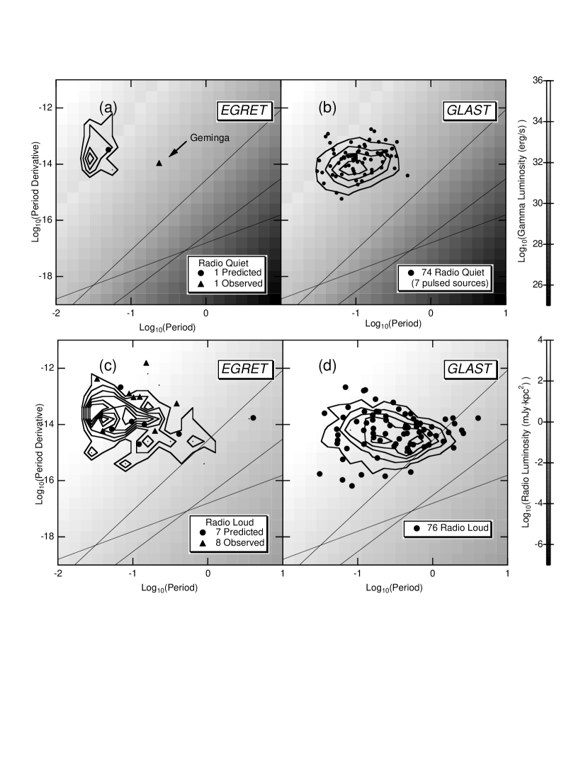
Figure 10: Distribution of radio-quiet (upper panels a and b) and radio-loud (lower panels c and d), $\gamma$-ray pulsars as a function of period derivative and period for EGRET and GLAST. Observed and simulated pulsars are represented by solid triangles and solid circles, respectively. The simulated distributions are for the case of no magnetic field decay and the presence of a pulsar death valley. Contours represent the distributions for a simulation of 10,000 radio pulsars in order to obtain smoother distributions. The background gray scale plots represent the average $\gamma$-ray (upper panels a and b) and radio (lower panels c and d) luminosities.

References

- (1)
- (2) Arzoumanian, Z., Chernoff, D.F., & Cordes, J.M., 2001, ApJ submitted.
- (3) Bailes, M. 1989, ApJ, 342, 917.
- (4) Baring, M. G. & Harding, A. K. 2000, AAS HEAD Meeting, Honolulu, HI, AAS Bull., 32, 1243.
- (5) Baring, M. G. & Harding, A. K. 2001, ApJ, 547, 929.
- (6) Bhattacharya, D., Wijers, R.A.M.J., Hartman, J.W., & Verbunt, F. 1992, A&AS, 254, 198.
- (7) Binney, J., & Tremaine, S. 1987, Galactic Dynamics, (Princeton University Press, New Jersey), 89.
- (8) Boyd, P.T. et al. 1995, ApJ, 448, 365.
- (9) Chen, K., & Ruderman, M.A. 1993, ApJ, 402, 264.
- (10) Cheng, K. S., Ho, C., & Ruderman, M. A. 1986, ApJ, 300, 500.
- (11) Cheng, K. S., & Zhang, L. 1998, ApJ, 498, 327.
- (12) Clifton, T.R. & Lyne, A.G. 1986, Nature, 320, 43.
- (13) Clifton, T.R, Lyne, A.G., Jones, A.W., McKenna, J., & Ashworth, M. 1992, MNRAS, 254, 177.
- (14) Cordes, J.M., & Chernoff, D.F. 1998, ApJ, 505, 315.
- (15) Daugherty, J. K., & Harding A. K. 1996, ApJ, 458, 278.
- (16) Dewey, R.J., & Cordes, J.M. 1997, ApJ, 321, 780.
- (17) Dewey, R.J., Taylor, J.H., Weisberg, J.M., & Stokes, G.H. 1985, ApJ, 294, L25.
- (18) Gehrels, N. et al. 2000, Nature, 404, 363.
- (19) Gil, J.A., & Han, J.L. 1996, ApJ, 458, 265.
- (20) Goldreich, P. & Reisenegger, A. 1992, ApJ, 395, 250.
- (21) Grenier, I.A. & Perrot, C. 1999, Proc. XXVI Int. Cosmic Ray Conf. Salt Lake City, 3, 476.
- (22) Gunn, J.E., & Ostriker, J.P. 1970, ApJ, 160, 979.
- (23) Hansen, B.M.S. & Phinney, E.S. 1997, MNRAS, 291, 569.
- (24) Harding, A. K. & Daugherty, J. K. 1999, A&AS, 120, 107.
- (25) Harding, A. K., & Muslimov, A. G. 1998, ApJ, 508, 328.
- (26) Harding, A. K., & Muslimov, A. G. 2001, ApJ, 556, 987.
- (27) Harding, A.K., & Zhang, B. 2001, ApJ, 548, L37.
- (28) Hartman, J.W. et al. 1997, A&A, 322, 477.
- (29) Hartman, R. et al. 1999, ApJ Supp., 123, 79.
- (30) Haslam, C.G.T., Salter, C.J., Stoffel, H., & Wilson, W.E. 1982, A&AS, 47,1.
- (31) Hirotani, K. & Shibata, S. 1999, MNRAS, 308, 67.
- (32) Johnston, S., Lyne, A.G., Manchester, R.N., Kniffen, D.A., D’Amico, N., Lim, J., & Ashworth, M. 1992, MNRAS, 255, 401.
- (33) Kaspi, V.M. et al. 1994, ApJ, 422, L83.
- (34) Kijak, J., & Gil, J. 1998, MNRAS, 299, 855.
- (35) Kuzmin, A.D. & Losovsky, B. Ya. 1997, IAU Circular, 6559.
- (36) Lorimer, D.R., Bailes, M., & Harrison, P.A. 1997, MNRAS, 289, 592.
- (37) Lyne, A.G. & Graham-Smith, F., 1998, Pulsar Astronomy, (Cambridge University Press New York), 9.
- (38) Lyne, A.G. et al. 1998, MNRAS, 295, 743.
- (39) Lyne, A.G., & Lorimer, D.R. 1994, Nature, 369, 127.
- (40) Lyne, A.G., Pritchard, R.S., & Smith, F.G. 1988, MNRAS, 233, 667.
- (41) Malofeev, V.M. & Malov, O.I. 1997, Nature, 389, 697.
- (42) Manchester, R.N. et al. 2001, MNRAS, in press.
- (43) Manchester, R.N. et al. 1978, MNRAS, 185, 409.
- (44) Manchester, R.N. et al. 1996, MNRAS, 279, 1235.
- (45) McLaughlin, M. A. & Cordes, J. M. 2000, ApJ, 538, 818.
- (46) Mollerach, S. & Roulet, E., 1997, ApJ, 479, 147.
- (47) Muslimov, A.G., & Harding, A.K. 1997, ApJ, 485, 735.
- (48) Muslimov, A.G., & Tsygan, A.I. 1992, MNRAS, 255, 61.
- (49) Narayan, R., & Ostriker, J.P. 1990, ApJ, 352, 222.
- (50) Nice, D.J., Taylor, J.H., & Fruchter, A.S. 1993, ApJ, 402, L49.
- (51) Paczyński, B. 1990, ApJ, 348, 485.
- (52) Press, W.H. et al. 1992, Numerical Recipes in C The Art of Scientific Computing, (Cambridge University Press New York), 136.
- (53) Prószyński, M., & Przybycién, D. 1984, in Birth and Evolution of Neutron Stars: Issues Raised by Millisecond Pulsars, ed. S.P. Reynolds and D.R. Stinebring (Green Bank: NRAO), p.151.
- (54) Rankin, J.M. 1993, ApJ, 405.
- (55) Romani, R. W. 1996, ApJ, 470, 469.
- (56) Romani, R. W., & Yadigaroglu, I.-A. 1995, ApJ, 438, 314.
- (57) Shapiro, S. L., & Teukolsky, S. A., 1983, Black Holes, White Dwarfs, and Neutron Stars The Physics of Compact Objects (John Wiley & Sons New York), 278.
- (58) Stokes, G.H., Segelstein, D.J., Taylor, J.H. & Dewey, R.J.1986, ApJ, 311, 694.
- (59) Sturner, S. J., Dermer, C. D. & Michel, F. C. 1995, ApJ, 445, 736.
- (60) Sturner, S. J., & Dermer, C. D. 1996a, A&AS, 120, 99.
- (61) Sturner, S. J., & Dermer, C. D. 1996b, ApJ, 461, 872.
- (62) Tauris, T. M. & Konar, S. 2001, astro-ph/0101531.
- (63) Taylor, J.H., & Cordes, J.M. 1993, ApJ, 411, 674.
- (64) Taylor, J.H., Manchester, R.N., & Lyne, A.G. 1993, ApJS, 88, 529.
- (65) Thompson, D. J., Harding, A.K., Hermsen, W., & Ulmer, M., 1997, in Proc. of 4th Compton Symposium, ed. C.D. Dermer, M.S. Strickman & J. Kurfess, p. 39.
- (66) Usov, V. V., & Melrose, D. B. 1995, Aust. J. Phys., 48, 571.
- (67) van den Heuvel, E. P. J. & van Paradijs, J. 1997, ApJ, 483, 399.
- (68) Vivekanand, M., & Narayan, R. 1981, J. Ap. Astr., 2, 315.
- (69) Yadigaroglu, I. A. & Romani, R. W. 1995, ApJ, 449, 211.
- (70) Zhang, B., & Harding, A. K. 2000, ApJ, 532, 1150.
- (71) Zhang, B., Harding, A. K., & Muslimov, A. G. 2000, ApJ, 531, L135.
- (72) Zhang, L., Zhang, Y. J. & Cheng, K. S. 2000, A & A, 357, 957.
- (73)