Local Group Velocity Versus Gravity:
The Coherence Function

Abstract

In maximum-likelihood analyses of the Local Group (LG) acceleration, the object describing nonlinear effects is the coherence function (CF), i.e. the cross-correlation coefficient of the Fourier modes of the velocity and gravity fields. We study the CF both analytically, using perturbation theory, and numerically, using a hydrodynamic code. The dependence of the function on $\Omega_{m}$ and the shape of the power spectrum is very weak. The only cosmological parameter that the CF is strongly sensitive to is the normalization $\sigma_{8}$ of the underlying density field. Perturbative approximation for the function turns out to be accurate as long as $\sigma_{8}$ is smaller than about $0.3$. For higher normalizations we provide an analytical fit for the CF as a function of $\sigma_{8}$ and the wavevector. The characteristic decoherence scale which our formula predicts is an order of magnitude smaller than that determined by Strauss et al.  This implies that present likelihood constraints on cosmological parameters from analyses of the LG acceleration are significantly tighter than hitherto reported.

1 Introduction

The dipole anisotropy of the Cosmic Microwave Background (CMB) temperature is widely believed to reflect, via the Doppler shift, the motion of the Local Group (LG) with respect to the CMB rest frame. When transformed to the barycentre of the LG, this motion is towards $(l,b)=(276^{\circ}\pm 3^{\circ},30^{\circ}\pm 2^{\circ})$, and of amplitude $v_{\rm LG}=627\pm 22$ $\hbox{km}\cdot\hbox{s}^{-1}$, as inferred from the 4-year COBE data (Lineweaver et al. 1996). Alternative models which assume that the dipole is due to a metric fluctuation (e.g., Paczyński & Piran 1990) have problems with explaining its observed achromaticity and the relative smallness of the CMB quadrupole.

An additional argument in favour of the kinematic interpretation of the CMB dipole is its remarkable alignment with the LG gravitational acceleration (or gravity), inferred from galaxy distribution. The acceleration on the LG, inferred from the IRAS PSCz survey points only $\sim 13^{\circ}$ away from the CMB dipole apex (Schmoldt et al. 1999; hereafter S99, Rowan-Robinson et al. 2000). The alignment between the two vectors is expected in the linear regime of gravitational instability (Peebles 1980), and under the hypothesis of linear biasing between galaxies and mass. The ratio of the amplitudes of the velocity and gravity vectors is then a measure of the quantity $\beta=\Omega_{m}^{0.6}/b$, where $\Omega_{m}$ and $b$ are the cosmological density of nonrelativistic matter and linear bias parameters, respectively. Therefore, comparisons between the LG gravity and the CMB dipole can serve not only as a test for the kinematic origin of the latter but also as a measure of $\beta$. Combined with other constraints on bias, they may yield an estimate of $\Omega_{m}$ itself.

However, the linear estimate of the LG velocity from a particular redshift survey will in general differ from its true velocity. The reasons are the finite volume of the survey, shot noise due to discrete sampling of the galaxy density field, redshift-space distortions and nonlinear effects. In a proper process of the LG velocity–gravity comparison, all these effects should be accounted for.

A commonly applied method of constraining cosmological parameters by the LG velocity–gravity comparison is a maximum-likelihood analysis, elaborated by several authors (especially by Strauss et al. 1992, hereafter S92; see also Juszkiewicz, Vittorio & Wyse 1990, Lahav, Kaiser & Hoffman 1990, S99). In this approach one maximizes the likelihood of particular values of cosmological parameters given the observed values of the LG velocity and gravitational acceleration. This enables one to constrain $\beta$ and the relative amount of power on large scales within the framework of a given cosmology.

The analysis of S92 constrained $\beta$ to lie between $0.4$ and $0.85$ (1 $\sigma$). The acceleration on the LG was derived there from the $1.2$ Jy survey of IRAS galaxies. S99 repeated this analysis, with the LG gravity inferred from the recently completed IRAS PSCz catalogue. This catalog contains almost three times more galaxies than its 1.2 Jy subsample. Still, the errorbars on $\beta$, obtained by S99 ($\beta=0.70^{+0.35}_{-0.2}$ at 1 $\sigma$), are not smaller than those obtained by S92. The volume surveyed is larger, shot noise is suppressed, but the errors remain big. Why? The authors blame nonlinear effects.

In nonlinear regime non-local nature of gravity is unveiled and the local relationship between the acceleration and velocity vectors is partly spoiled. In other words, the nonlinear velocity–gravity relation at a given point has scatter. As a result, the precision of determining $\beta$ by the method described above is fundamentally limited, regardless how well we can measure the LG gravity (and velocity).

This argument sounds reasonable. However, if nonlinear effects are so strong, why is the misalignment angle between the LG gravity and velocity so small? Doesn’t it actually suggest otherwise? This motivated us to reanalyze nonlinear effects in the LG velocity–gravity comparison.

In a maximum-likelihood analysis, a proper object describing nonlinear effects is the coherence function (hereafter CF), i.e. the cross-correlation coefficient of the Fourier modes of the gravity and velocity fields (see S92 for details). S92 devised a formula for the CF, calibrating it so as to fit the results of N-body simulations of a standard CDM cosmology. They adopted this form of the function in all subsequent analyses, thus ignoring any possible dependence it may have on the shape of the power spectrum and its normalization. A similar approach was adopted by S99, who followed ‘the S92 assumption that the CF does not change appreciably with the background cosmology’. S99 applied the same form of the function in two different cosmological models: spatially flat CDM cosmologies with respectively zero and non-zero ($\Omega_{\Lambda}=0.7$) cosmological constant. The adopted value for the spectral parameter $\Gamma$ was $0.25$ and the spectra were cluster-normalized, so they had different values of $\sigma_{8}$ (r.m.s. mass fluctuations on the 8 $h^{-1}\,\hbox{Mpc}$ scale).

By definition, on large enough, linear scales the CF is unity. On smaller scales we expect it to begin to depart from this value. The scale of departure marks a characteristic scale at which the non-local nature of gravity can no longer be ignored. Non-locality of the fields must be somehow correlated with their non-linearity, because it does not appear for linear fields. Since in more evolved models the nonlinearity scale is larger, it is natural to expect the CF to depend on the normalization of the underlying power spectrum. If this is indeed the case, then this dependence should be modelled, to be accounted for in future LG velocity–gravity comparisons. The dependence on other cosmological parameters should also be studied. This is the aim of the present paper. It is organized as follows. In Section 2 we calculate the CF perturbatively. In Section 3 we describe the numerical simulations which we use to estimate the CF numerically. Results of the simulations are presented in Section 4. In particular, we compare the analytical estimates with the numerical estimates of the CF. In Section 5 we show that the CF significantly affects the estimation of cosmological parameters in maximum-likelihood analyses of the LG acceleration. Moreover, we constrain the CF in an alternative way, adopted by S92. Summary and conclusions are in Section 6.

2 Analytical calculations

The CF is defined as

$$C({\bf k})=\frac{\langle{\bf g}_{\bf k}\cdot{\bf v}_{\bf k}^{\star}\rangle}{\langle|{\bf g}_{\bf k}|^{2}\rangle^{1/2}\langle|{\bf v}_{\bf k}|^{2}\rangle^{1/2}}\,,$$ (1)

where ${\bf g}_{\bf k}$ and ${\bf v}_{\bf k}$ are the Fourier components of the gravity and velocity fields, and $\langle\ldots\rangle$ means the ensemble averaging. (Note that the definition of S92 lacks the complex conjugate sign.) The function can be interpreted as the cross-correlation coefficient of the Fourier modes of the gravity and velocity fields. It is important for the LG gravity–velocity comparisons, because it appears in the likelihood function for the LG velocity and acceleration (see Section 5). As argued in the Introduction, the CF is also interesting in its own right – it carries information about non-locality, and indirectly about non-linearity, of the fields. In this section we calculate the CF for the fields which are weakly non-linear.

By definition, $C({\bf k})$ is invariant to scaling of ${\bf g}_{\bf k}$ and ${\bf v}_{\bf k}$ by an arbitrary constant. We are then free to choose the fields scaled so as to fulfill the following equations:

$$\nabla\cdot{\bf g} = \delta\,,$$ (2)

$$\nabla\cdot{\bf v} = \theta\,.$$ (3)

Here, $\delta$ is the mass density contrast and $\theta$ is the velocity divergence, scaled in such a way that in the linear regime $\theta=\delta$.

The gravity field is strictly irrotational. Hence

$${\bf g}_{\bf k}=\frac{i{\bf k}}{k^{2}}\delta_{\bf k}\,,$$ (4)

where $\delta_{\bf k}$ is the Fourier transform of the density contrast. Due to Kelvin’s circulation theorem, the cosmic velocity field is vorticity-free as long as there is no shell crossing. Since appreciable shell crossing does not occur for weakly nonlinear fields, we have

$${\bf v}_{\bf k}=\frac{i{\bf k}}{k^{2}}\theta_{\bf k}\,,$$ (5)

where $\theta_{\bf k}$ is the Fourier transform of the velocity divergence. Using equations (4) and (5) we obtain

$$C({\bf k})=\frac{\langle\delta_{\bf k}{\theta_{\bf k}}^{\!\!\star}\rangle}{\langle\delta_{\bf k}{\delta_{\bf k}}^{\!\!\star}\rangle^{1/2}\langle\theta_{\bf k}{\theta_{\bf k}}^{\!\!\star}\rangle^{1/2}}\,.$$ (6)

We assume here that the density and velocity divergence fields are homogeneous and isotropic random fields. For such fields, the CF depends only on the magnitude of the wavevector. Furthermore, the density and velocity divergence are real fields, what implies that ${\delta_{\bf k}}^{\!\!\star}=\delta_{-{\bf k}}$, and similarly for the velocity divergence. All this implies that the CF is a real function, as follows. Namely, we have $C({\bf k})=C(-{\bf k})$, hence $\langle\delta_{\bf k}{\theta_{\bf k}}^{\!\!\star}\rangle=\langle\delta_{-{\bf k}}{\theta_{-{\bf k}}}^{\!\!\star}\rangle=\langle{\delta_{{\bf k}}}^{\!\!\star}\theta_{\bf k}\rangle={\langle\delta_{\bf k}{\theta_{\bf k}}^{\!\!\star}\rangle}^{\star}$. Therefore, $C(k)=[C(k)]^{\star}$, that is $C(k)$ is real. We may then cast it to an explicitly real form:

$$C(k)=\frac{\langle\delta_{\bf k}{\theta_{\bf k}}^{\!\!\star}\rangle+\langle{\delta_{{\bf k}}}^{\!\!\star}\theta_{\bf k}\rangle}{2\langle\delta_{\bf k}{\delta_{\bf k}}^{\!\!\star}\rangle^{1/2}\langle\theta_{\bf k}{\theta_{\bf k}}^{\!\!\star}\rangle^{1/2}}\,.$$ (7)

This formula is a good approximation to the CF as long as the velocity field has negligible vorticity. N-body simulations (Bertschinger & Dekel 1989, Mancinelli et al. 1994, Pichon & Bernardeau 1999) show that even in the case of fully nonlinear fields, the generated vorticity is small.

We now expand $\delta_{\bf k}$ and $\theta_{\bf k}$ in perturbative series: $\delta_{\bf k}=\delta_{\bf k}^{(1)}+\delta_{\bf k}^{(2)}+\delta_{\bf k}^{(3)}+\ldots$, and similarly $\theta_{\bf k}=\theta_{\bf k}^{(1)}+\theta_{\bf k}^{(2)}+\theta_{\bf k}^{(3)}+\ldots$. Since in the linear regime $\theta=\delta$, we have $\theta_{\bf k}^{(1)}=\delta_{\bf k}^{(1)}$. We assume here that the initial (linear) density fluctuation field is a Gaussian random field. For such a field, all odd-order moments of the density contrast and of the velocity divergence vanish. Then, $\langle\delta_{\bf k}{\theta_{\bf k}}^{\!\!\star}\rangle=\bigl{\langle}\delta_{\bf k}^{(1)}{\theta_{\bf k}^{(1)}}^{\star}\bigr{\rangle}+\bigl{\langle}\delta_{\bf k}^{(1)}{\theta_{\bf k}^{(3)}}^{\star}\bigr{\rangle}+\bigl{\langle}\delta_{\bf k}^{(3)}{\theta_{\bf k}^{(1)}}^{\star}\bigr{\rangle}+\bigl{\langle}\delta_{\bf k}^{(2)}{\theta_{\bf k}^{(2)}}^{\star}\bigr{\rangle}+{\cal O}\left(\sigma^{6}\right)$, where $\sigma^{2}\equiv\langle\delta^{2}\rangle$, and similarly for other terms appearing in formula (7). Up to the leading order corrective term, this expansion yields

$$C(k)=1-\frac{\Bigl{\langle}\bigl{|}\delta_{\bf k}^{(2)}-\theta_{\bf k}^{(2)}\bigr{|}^{2}\Bigr{\rangle}}{2(2\pi)^{3}P(k)}\,.$$ (8)

Here, $P(k)$ is the linear power spectrum, defined as $(2\pi)^{-3}\bigl{\langle}\delta_{\bf k}^{(1)}{\delta_{\bf k}^{(1)}}^{\star}\bigr{\rangle}$.

The above formula is somewhat similar to that describing weakly nonlinear corrections to the evolution of the power spectrum (Makino et al. 1992, Jain & Bertschinger 1994). There is, however, also an important difference. Namely, all terms of the sort $\bigl{\langle}\alpha_{\bf k}^{(1)}{\beta_{\bf k}^{(3)}}^{\star}\bigr{\rangle}$, where $\alpha$ and $\beta$ stand for either $\delta$ or $\theta$, have remarkably cancelled out. In other words, unlike the weakly nonlinear power spectrum, the weakly nonlinear CF is constructed solely from second-order terms.

To proceed further, we need the forms of $\delta_{\bf k}^{(2)}$ and $\theta_{\bf k}^{(2)}$. Second-order solutions for the density contrast and (scaled) velocity divergence have been shown to depend extremely weakly on $\Omega_{m}$ and $\Omega_{\Lambda}$ (Bouchet et al. 1992, Bouchet et al. 1995, Bernardeau et al. 1995). This is also true for higher orders (see App. B.3 of Scoccimarro et al. 1998). Here we neglect the weak $\Omega$-dependence. Then (Goroff et al. 1986)

$$\delta_{\bf k}^{(2)}=\!\int\frac{{\rm d}^{3}k_{1}{\rm d}^{3}k_{2}}{(2\pi)^{3}}\delta_{D}({\bf k}_{1}+{\bf k}_{2}-{\bf k})J^{(2)}({\bf k}_{1},{\bf k}_{2})\,\delta_{{\bf k}_{1}}^{(1)}\delta_{{\bf k}_{2}}^{(1)}$$ (9)

and

$$\theta_{\bf k}^{(2)}=\!\int\frac{{\rm d}^{3}k_{1}{\rm d}^{3}k_{2}}{(2\pi)^{3}}\delta_{D}({\bf k}_{1}+{\bf k}_{2}-{\bf k})K^{(2)}({\bf k}_{1},{\bf k}_{2})\,\delta_{{\bf k}_{1}}^{(1)}\delta_{{\bf k}_{2}}^{(1)},$$ (10)

where $\delta_{D}$ is the Dirac delta,

$$J^{(2)}({\bf k}_{1},{\bf k}_{2})=\frac{5}{7}+\frac{2}{7}\frac{({\bf k}_{1}\cdot{\bf k}_{2})^{2}}{k_{1}^{2}k_{2}^{2}}+\frac{({\bf k}_{1}\cdot{\bf k}_{2})}{2}\left(\frac{1}{k_{1}^{2}}+\frac{1}{k_{2}^{2}}\right)$$ (11)

and

$$K^{(2)}({\bf k}_{1},{\bf k}_{2})=\frac{3}{7}+\frac{4}{7}\frac{({\bf k}_{1}\cdot{\bf k}_{2})^{2}}{k_{1}^{2}k_{2}^{2}}+\frac{({\bf k}_{1}\cdot{\bf k}_{2})}{2}\left(\frac{1}{k_{1}^{2}}+\frac{1}{k_{2}^{2}}\right)\!.$$ (12)

Hence we have

$$\delta_{\bf k}^{(2)}-\theta_{\bf k}^{(2)}=\!\int\frac{{\rm d}^{3}k_{1}{\rm d}^{3}k_{2}}{(2\pi)^{3}}\delta_{D}({\bf k}_{1}+{\bf k}_{2}-{\bf k})L({\bf k}_{1},{\bf k}_{2})\,\delta_{{\bf k}_{1}}^{(1)}\delta_{{\bf k}_{2}}^{(1)}\!,$$ (13)

where

$$L({\bf k}_{1},{\bf k}_{2})=\frac{2}{7}\left[1-\left(\frac{{\bf k}_{1}\cdot{\bf k}_{2}}{k_{1}k_{2}}\right)^{2}\right].$$ (14)

To determine $\bigl{\langle}\bigl{|}\delta_{\bf k}^{(2)}-\theta_{\bf k}^{(2)}\bigr{|}^{2}\bigr{\rangle}$, we need to evaluate the four-point correlations of the linear density field $\delta_{{\bf k}}^{(1)}$. For a Gaussian random field,

$$\left\langle\delta_{{\bf k}_{1}}^{(1)}\delta_{{\bf k}_{2}}^{(1)}\delta_{{\bf k}_{3}}^{(1)}\delta_{{\bf k}_{4}}^{(1)}\right\rangle=$$

$$(2\pi)^{6}\delta_{D}({\bf k}_{1}+{\bf k}_{2})\delta_{D}({\bf k}_{3}+{\bf k}_{4})P(k_{1})P(k_{3})+$$

$$(2\pi)^{6}\delta_{D}({\bf k}_{1}+{\bf k}_{3})\delta_{D}({\bf k}_{2}+{\bf k}_{4})P(k_{1})P(k_{2})+$$

$$(2\pi)^{6}\delta_{D}({\bf k}_{1}+{\bf k}_{4})\delta_{D}({\bf k}_{2}+{\bf k}_{3})P(k_{1})P(k_{2})\,.$$ (15)

Using this property, it is a standard perturbative calculation to show that

$$\left\langle\bigl{|}\delta_{\bf k}^{(2)}-\theta_{\bf k}^{(2)}\bigr{|}^{2}\right\rangle=2\!\int{\rm d}^{3}qP(q)P(|{\bf k}-{\bf q}|)L^{2}({\bf q},{\bf k}-{\bf q})\,,$$ (16)

with $L$ given by equation (14).

Note that $J^{(2)}$ and $K^{(2)}$ have first-order poles as $k_{1}\to 0$ or $k_{2}\to 0$ for fixed ${\bf k}$: $J^{(2)}\sim K^{(2)}\sim(1/2)\cos\vartheta(k_{1}/k_{2}+k_{2}/k_{1})$, where $\vartheta$ is the angle between ${\bf k}_{1}$ and ${\bf k}_{2}$. However, in the expression (13) for $\delta_{\bf k}^{(2)}-\theta_{\bf k}^{(2)}$ they cancel out: the function $L$ has no poles. This results in significant simplification of the integrand in equation (16).

Using formula (8) we obtain

$$C(k)=1-P^{-1}(k)\!\int\!\frac{{\rm d}^{3}q}{(2\pi)^{3}}P(q)P(|{\bf k}-{\bf q}|)L^{2}({\bf q},{\bf k}-{\bf q})\,.$$ (17)

Now we write the integral in spherical coordinates $q$, $\vartheta$ and $\phi$, the magnitude, polar angle, and azimuthal angle, respectively, of the wavevector ${\bf q}$. Then with the external wavevector ${\bf k}$ aligned along the $z$-axis the integral over $\phi$ is trivial and simplifies $\int{\rm d}^{3}q$ to the form $2\pi\int{\rm d}qq^{2}\int{\rm d}\cos\vartheta$. Furthermore, we have

$$L^{2}({\bf q},{\bf k}-{\bf q})=\frac{4}{49}\frac{\left(1-\mu^{2}\right)^{2}}{\left[1+(q/k)^{2}-2(q/k)\mu\right]^{2}}\,,$$ (18)

where $\mu=\cos\vartheta$. This suggests a change of variables $s\equiv q/k$. Performing this finally yields

$$1-C(k)\!\!\!\! = \!\!\!\!\frac{4k^{3}}{49(2\pi)^{2}P(k)}\int_{k_{min}/k}^{k_{max}/k}{\rm d}s\,s^{2}P(ks)\int_{-1}^{1}{\rm d}\mu\times$$ (19)

$$\!\!\!\!P[k(1+s^{2}-2s\mu)^{1/2}]\,F(s,\mu)\,,$$

with

$$F(s,\mu)=\frac{\left(1-\mu^{2}\right)^{2}}{(1+s^{2}-2s\mu)^{2}}\,.$$ (20)

The quantities $k_{min}$ and $k_{max}$ are the cutoffs of the power spectrum. Physically, they are related to the effective depth of the survey, from which the specific spectrum is extracted, and the virialization scale, respectively. (For $k>k_{max}$ perturbative expansion breaks down.) In numerical simulations, $k_{min}$ and $k_{max}$ are determined by the simulation box size and elemental cell size, respectively. Details will be given in the next Section.

Given the linear spectrum $P(k)$, equation (19) provides the second-order correction to the linear value of the CF. Results for the PSCz spectrum and for the standard-CDM spectrum are presented in Section 4.

3 Numerical simulations

Following Peebles (1987), instead of using a N-body scheme we model cold dark matter as a pressureless cosmic fluid. Using the Eulerian code CPPA (Cosmological Pressureless Parabolic Advection, see Kudlicki, Plewa & Różyczka 1996, Kudlicki et al. 2000, Kudlicki et al. 2001b) we solve its dynamical equations on a uniform grid fixed in comoving coordinates. The main improvements of CPPA over the original Peebles’ code are parabolic density and velocity profiles, variable timestep, periodic boundary conditions and a flux interchange procedure, implemented as an approximation to the solution of the Boltzmann equation.

We chose to use a grid-based code rather than a $N$-body code because it directly produces a volume-weighted velocity field. This is important because in the definition of the CF, equation (1), the velocity field is volume-weighted, not mass-weighted. Moreover, the field is evenly sampled, which is convenient for FFT techniques.

The linear velocity depends on the cosmological constant ($\Omega_{\Lambda}$) very weakly (e.g. Lahav et al. 1991); this also holds for higher orders (see Bouchet et al. 1995, Appendix B.3 of Scoccimarro et al. 1998 and Nusser & Colberg 1998). Therefore, it was a good approximation to assume $\Omega_{\Lambda}=0$ in our models. We have thus studied two zero-$\Lambda$ models with $\Omega_{m}=1$ and $\Omega_{m}=0.3$, assuming Gaussian initial conditions. The parameters of the runs are given in Table 1.

Table 1: Parameters of the runs displayed in Figure 1. The acronym l-l stands for ‘low $N^{3}$, low $k_{\rm Nq}$’, h-l stands for ‘high $N^{3}$, low $k_{\rm Nq}$’, and h-h stands for ‘high $N^{3}$, high $k_{\rm Nq}$’.

run	grid	box size [$h^{-1}\rm Mpc$]	$k_{\rm Nq}~{}[h\,{\rm Mpc}^{-1}]$
l-l	$64^{3}$	50	4.
h-l	$128^{3}$	100	4.
h-h	$128^{3}$	50	8.

To make the simulated gravitational field as close as possible to that inferred from the IRAS PSCz survey, the mass power spectrum that we adopted was that estimated for the PSCz galaxies (Sutherland et al. 1999):

$$P(k) = \frac{Bk}{\{1+[ak+(bk)^{3/2}+(ck)^{2}]^{\nu}\}^{2/\nu}}$$ (21)

$$a = 6.4/\Gamma{\,h^{-1}\rm Mpc}\,,~{}~{}~{}b=3.0/\Gamma{\,h^{-1}\rm Mpc}\,,$$

$$c = 1.7/\Gamma{\,h^{-1}\rm Mpc}\,,~{}~{}~{}\nu=1.13\,,$$

with $\Gamma=0.2$ as best fitted value. The power spectrum employed in simulations is effectively truncated at both large (corresponding to the lower cutoff $k_{min}$) and small (corresponding to the upper cutoff $k_{max}$) scales. Specifically, $k_{min}=2\pi/L$, where $L$ is the simulation box size, and $k_{max}=k_{\rm Nq}=(N/2)k_{min}$. Here, $k_{\rm Nq}$ is the so-called Nyquist wavevector and $N^{3}$ is the grid size.

To normalize the power spectrum we used the observed local abundance of galaxy clusters. The present value of $\sigma_{8}$, labelled $\sigma_{8,0}$, is a function of $\Omega_{m}$ and for the case of $\Omega_{\Lambda}=0$ it is estimated by the relation (Eke, Cole & Frenk 1996)

$$\sigma_{8,0}=(0.52\pm 0.04)\Omega_{m}^{-0.46+0.10\Omega_{m}}\,.$$ (22)

This relation changes only slightly with the shape of the power spectrum. It is also very similar for the case of non-zero $\Omega_{\Lambda}$, flat models ($\Omega_{\Lambda}=1-\Omega_{m}$). For $\Omega_{m}=1$, $\sigma_{8,0}\simeq 0.52$, while for $\Omega_{m}=0.3$, $\sigma_{8,0}\simeq 0.87$.

4 Results

Firstly, we tested the dependence of the results on resolution. For this purpose we performed three simulations of an $\Omega_{m}=1$ Universe with the PSCz power spectrum (see Table 1). The runs l-l and h-l have the same spatial resolution but different grid resolutions, while the run h-h has higher spatial resolution. In Figure 1, we present the temporal evolution of the CF. Specifically, we show it for 3 values of $\sigma_{8}$: $0.1$, $0.3$, and $0.52$. As expected, the results of runs l-l and h-l do not differ significantly. In contrast to the run h-l, the run l-l has no modes corresponding to the scales greater than $50$ $h^{-1}\,\hbox{Mpc}$. These scales, however, are well in the linear regime, so $C=1$ to good accuracy.

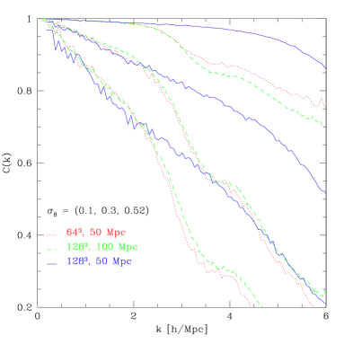
Figure 1: The CF for three values of $\sigma_{8}$, for three Einstein–de Sitter simulations with different resolutions. (Their parameters are given in Table 1.) Dotted lines show the results of run l-l, dashed lines h-l, and solid lines h-h. The CF is similar for runs l-l and h-l. For $k<2~{}h\,{\rm Mpc}^{-1}$, it is similar for all runs. For each run, the function bends down at $k\simeq 0.5k_{\rm Nq}$.

In grid simulations, the largest wavevector is the Nyquist wavevector, corresponding to the Nyquist wavelength, i.e., the smallest wavelength, of two cells. Its values for the three runs are given in the last column of Table 1. Fourier modes with $k>k_{\rm Nq}$ do not have physical meaning. Inspection of Figure 1, however, shows that the CF bends down already at $k\simeq 0.5k_{\rm Nq}$. Such a scaling of the bending point with the Nyquist wavevector strongly suggests that this is a resolution effect. Given the similarity of the three curves for $k<2~{}h\,{\rm Mpc}^{-1}$, we can expect the CF to be free of resolution effects up to $k\simeq 0.5k_{\rm Nq}$, for any grid.

Next, we test the perturbative approximation for the CF. In Figure 2, we show the CF from simulations with the grid $128^{3}$ and the box-size of $50$ $h^{-1}\,\hbox{Mpc}$, for wavevectors up to $0.5k_{\rm Nq}=4.0~{}h\,{\rm Mpc}^{-1}$. Dotted lines are for $\Omega_{m}=1.0$, dashed for $\Omega_{m}=0.3$, while solid show predictions of perturbation theory for $\Omega_{m}=1.0$, according to formula (19). (We numerically evaluate the integral in this formula.) The CF depends on $\Omega_{m}$ very weakly. Moreover, except for the highest $k$-values, it is well predicted by the second-order approximation, as long as $\sigma_{8}$ is smaller than $\sim 0.3$. We have checked that for $\sigma_{8}<0.3$ the quantity $1-C(k)$ scales approximately like $\sigma_{8}^{2}$, as predicted by equation (19) (the normalization of $P(k)$ is proportional to $\sigma_{8}^{2}$). For higher values of $\sigma_{8}$, the second-order approximation overestimates the deviation of $C$ from the linear value, unity. This behaviour is similar to the nonlinear evolution of the power spectrum, overestimated by second-order terms (Jain & Bertschinger 1994).

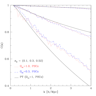
Figure 2: The CF for simulations $128^{3}$ with the box-size of $50$ $h^{-1}\,\hbox{Mpc}$. Dotted lines are for $\Omega_{m}=1.0$, dashed for $\Omega_{m}=0.3$, and solid show predictions of perturbation theory for $\Omega_{m}=1.0$, according to formula (19). The CF depends on $\Omega_{m}$ very weakly. For $\sigma_{8}\leq 0.3$, it is well predicted by the second-order approximation, except for the highest values of the wavevector.

To describe the CF for $\sigma_{8}>0.3$, we analyzed it for 23 output times of the high-resolution simulation h-h, corresponding to the values of $\sigma_{8}$ in the range $0.3<\sigma_{8}<1.0$. We found that the $\sigma_{8}$-dependence of $C$ can be well fitted as

$$C(k)=\exp{(-ak)}\,,$$ (23)

where

$$a=\left\{\begin{array}[]{ll}0.757~{}\sigma_{8}^{2}&\mbox{for $\sigma_{8}\leq 0.3$}\,,\\ -0.059+0.423~{}\sigma_{8}&\mbox{for $0.3<\sigma_{8}\leq 1.0$}\,.\end{array}\right.$$ (24)

In Figure 3 we show the CF from the simulation h-h, for $\sigma_{8}$ given by the cluster normalization. (Having shown very weak dependence of the function on $\Omega_{m}$, in this plot we present the results of Einstein–de Sitter simulations only, which are simpler to evolve numerically.) In particular, in this figure the dotted line for $\sigma_{8}=0.52$ corresponds to the lowest solid line in Figure 1. The fits are good; we have checked that for other values of $\sigma_{8}$ they are as good as those shown here.

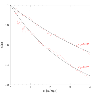
Figure 3: The coherence function for cluster-normalized cosmological models. Dotted lines show the function from the numerical simulation h-h, while solid ones are the fits according to formula (23).

To test the dependence of the CF on the underlying power spectrum, we performed a $64^{3}$ simulation with the standard CDM spectrum ($\Gamma=0.5$). The box-size was $50$ $h^{-1}\,\hbox{Mpc}$, so $0.5\,k_{\rm Nq}=2$. The results are shown in Figure 4. Solid lines are drawn according to our fit (eq. 23), obtained for the PSCz spectrum, while dotted lines are from the simulation. A good agreement between them apparent in the figure implies that the dependence of the CF on the power spectrum is very weak, at least for a CDM-like family of the spectra.

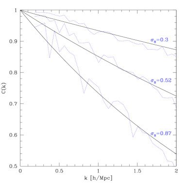
Figure 4: The coherence function from a simulation with the standard-CDM power spectrum (dotted) versus our formula (23), obtained for the PSCz spectrum (solid).

The CF has been modelled by S92, who calibrated it so as to fit the results of N-body simulations of a standard CDM cosmology. In Figure 5 we show S92’s prediction for $C$, as well as our predictions, for the standard CDM power spectrum and $\sigma_{8}$ normalization of S92 ($0.625$). The discrepancy of our results with the formula of S92 is drastic! Instead of a characteristic decoherence scale of $4.5$ $h^{-1}\,\hbox{Mpc}$ (S92), our formula (23) suggests a fraction of a megaparsec. We will comment on that in the summary.

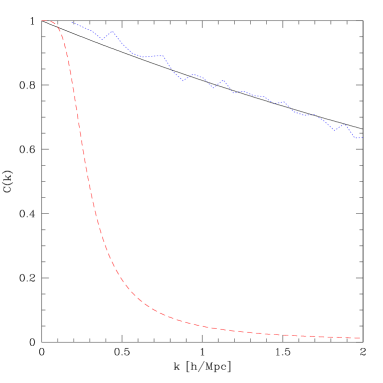
Figure 5: The coherence function for a standard-CDM cosmological model with $\sigma_{8}=0.625$. The dotted line shows the function from our standard-CDM simulation, while the solid one is the fit according to formula (23). The dashed line is the formula (18) of S92, with $r_{c}=4.5$ $h^{-1}\,\hbox{Mpc}$.

5 From coherence to probability contours

The aim of this Section is twofold. Firstly, we show that the CF is very important in the analyses of the LG acceleration, because, together with other factors, it determines the relative likelihood of different cosmological models. Secondly, we show that the probability distribution for the LG acceleration amplitude and the misalignment angle, resulting from our estimate of the CF, is consistent with that obtained from mock IRAS catalogs, constructed by S92. In contrast, adopting S92’s formula for the function results in a distribution which is too broad. Here we only outline the necessary formalism; for more details the reader is referred to S92 and Chodorowski & Cieciela̧g (2001).

Let $f({\bf g},{\bf v})$ denote the probability density distribution for observing particular values of the LG gravity and velocity, given some assumed CDM cosmological model. The model is fully specified by the value of $\beta$, the power spectrum shape parameter $\Gamma$, and the normalization $\sigma_{8}$. Due to Bayes theorem, it is possible to evaluate from $f$ the relative likelihood, ${\cal L}$, of different models ($\beta$, $\Gamma$, $\sigma_{8}$). The likelihood function is usually defined as

$${\cal L}=f\,.$$ (25)

Here, the observed values of the Local Group velocity and gravity are inserted in $f$ and serve as constraints on cosmological parameters.

As a functional form of $f$, S92 and S99 adopt a multivariate Gaussian. This assumption has support from numerical simulations (Koffman et al. 1994, Kudlicki et al. 2001a), where the measured nongaussianity of ${\bf g}$ and ${\bf v}$ is small. This is rather natural to expect since, e.g., gravity is an integral of density over effectively a large volume, so the central limit theorem can at least partly be applicable (but see Catelan & Moscardini 1994). However, the approximate Gaussianity of ${\bf g}$ and ${\bf v}$ by no means implies that the fields are linear. In contrast, the above considerations suggest a Gaussian approximation for the form of $f$, but with the covariance matrix calculated accounting for the nonlinear effects.

After some algebra (see e.g. Juszkiewicz et al. 1990), the joint distribution for ${\bf g}$ and ${\bf v}$ can be cast to the form:

$$f({\bf g},{\bf v})=\frac{(1-r^{2})^{-3/2}}{(2\pi)^{3}\sigma_{g}^{3}\sigma_{v}^{3}}\exp\left[-\frac{x^{2}+y^{2}-2r\mu xy}{2(1-r^{2})}\right]\,,$$ (26)

where $\sigma_{g}$ and $\sigma_{v}$ denote the r.m.s. values of a single spatial component of gravity and velocity, respectively. From statistical isotropy, $\sigma_{g}^{2}=\langle{\bf g}\cdot{\bf g}\rangle/3$, and $\sigma_{v}^{2}=\langle{\bf v}\cdot{\bf v}\rangle/3$. Next, $({\bf x},{\bf y})=({\bf g}/\sigma_{g},{\bf v}/\sigma_{v})$, and $\mu=\cos\theta$ with $\theta$ being the misalignment angle between ${\bf g}$ and ${\bf v}$. Finally, $r$ is the cross-correlation coefficient of $g_{i}$ with $v_{i}$, where $g_{i}$ ($v_{i}$) denotes an arbitrary spatial component of ${\bf g}$ (${\bf v}$). From isotropy,

$$r=\frac{\langle{\bf g}\cdot{\bf v}\rangle}{\langle g^{2}\rangle^{1/2}\langle v^{2}\rangle^{1/2}}\,.$$ (27)

Also from isotropy,

$$\langle x_{i}y_{j}\rangle=r\,\delta_{ij}\,,$$ (28)

where $\delta_{ij}$ denotes the Kronecker delta. In other words, there are no cross-correlations between different spatial components.

In the limit of linear fluctuations and with perfect sampling of the density field, the distribution (26) reduces to $\delta_{D}({\bf x}-{\bf y}){\cal N}_{3}({\bf v})$, where ${\cal N}_{3}$ denotes a tri-variate normal distribution. In a real world, there are nonlinear effects (NL), as well as finite-volume effects (FV), which make the cross-correlation coefficient deviate from unity. In a related paper (Chodorowski & Cieciela̧g 2001) we will show that $r$ can be approximately written as

$$r=r_{\rm NL}\cdot r_{\rm FV}\,,$$ (29)

i.e. that the contributions to $r$ from nonlinear effects separate from those from finite volume. In the present paper we study nonlinear effects. The cross-correlation coefficient due to them is

$$r_{\rm NL}=\frac{\int_{0}^{\infty}C(k)W_{g}(k)W_{v}(k)P(k)\,{\rm d}k}{\int_{0}^{\infty}W_{g}(k)W_{v}(k)P(k)\,{\rm d}k}\,.$$ (30)

Here $W_{g}$ and $W_{v}$ are the observational filters of ${\bf g}$ and ${\bf v}$ (for details see S92). Thus, nonlinear effects enter into the correlation coefficient of the joint distribution function via the CF. In the linear regime $C=1$ and, if we neglect other effects, $r=1$. Since the distribution function is directly related to the likelihood of different world models (eq. 25), in analyses of the LG acceleration, the CF affects the estimation of cosmological parameters.

In equation (30) the CF is multiplied by the windows through which the gravity and velocity of the LG are measured. Therefore, smoothing effectively filters out the high-$k$ tail of the coherence function. It is instructive to write

$$1-r_{\rm NL}=\frac{\int_{0}^{\infty}\left[1-C(k)\right]W_{g}(k)W_{v}(k)P(k)\,{\rm d}k}{\int_{0}^{\infty}W_{g}(k)W_{v}(k)P(k)\,{\rm d}k}\,;$$ (31)

the stronger the deviation of $C$ from unity so is the deviation of $r_{\rm NL}$. In Figure 6 we plot the integrand $[1-C(k)]W_{g}(k)W_{v}(k)P(k)$ as a function of $k$. (Strictly speaking, we plot the function $[1-C(k)]W_{g}(k)W_{v}(k)kP(k)$, because the $k$-axis is logarithmic.) Here $C(k)$ is given by our fit (eq. 23), $P(k)$ is the spectrum of the PSCz galaxies, and the velocity window is that introduced by S92, with a small-scale cutoff, $r_{min}=1$ $h^{-1}\,\hbox{Mpc}$, to reflect the finite size of the LG. The gravity window is either the standard IRAS window with a small-scale smoothing $r_{s}=5$ $h^{-1}\,\hbox{Mpc}$ (S92), or equal to the velocity window. The first case corresponds to the present situation, where the inferred LG gravity is commonly smoothed with the standard IRAS window, and results in the dashed curve. The second case describes an ideal situation, where the galaxy distribution around the LG is sampled so densely that there is no need to smooth its gravity beyond the size of the LG. That case results in the dotted curve. We see from the figure that at present it is sufficient to know the behaviour of the CF up to at most $k=2~{}h\,{\rm Mpc}^{-1}$, and it will never become necessary to know it for $k>4~{}h\,{\rm Mpc}^{-1}$. This is why we have set up the resolution of the h-h simulation in such a way that $0.5\,k_{\rm Nq}=4~{}h\,{\rm Mpc}^{-1}$ (Section 4).

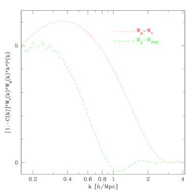
Figure 6: The integrand in the numerator of the right-hand side of equation (31) as a function of the wavevector. Since the $k$-axis is logarithmic, the ordinate is multiplied by and extra power of $k$, so equal areas under the function correspond to equal contributions to the deviation of the correlation coefficient from unity. Units of the ordinate axis are arbitrary.

In contrast to our approach, S92 did not determine the CF from its definition. Instead, using standard CDM N-body simulations, they created mock IRAS catalogs for ‘observers’ (N-body points) selected with similar properties to those of the LG (primarily the velocity). For each of these observers, S92 computed the IRAS acceleration of the LG, as the filter $W_{g}$ using the so-called standard IRAS window. They then matched the resulting distribution for the amplitude of ${\bf g}$ and the misalignment angle with the probability contours resulting from a formula following from equation (26). Since the LG velocity was considered by S92 as a constraint, we need the conditional probability density function $f({\bf g}|{\bf v})$. It readily results from formula (26):

$$f({\bf g}|{\bf v})=(2\pi)^{-3/2}\sigma_{g}^{-3}(1-r^{2})^{-3/2}\exp\left[-\frac{({\bf x}-r{\bf y})^{2}}{2(1-r^{2})}\right]$$ (32)

(Juszkiewicz et al. 1990). The distribution for $g$ and $\theta$ results from the above formula by multiplying it by $2\pi g^{2}\sin\theta$.

The approach adopted by S92 implies that the finite volume effects are also present, so they should also be modelled. We did so, and the results are presented in Figures 7 and 8. Specifically, in both figures the scattered points are the distribution for $g$ and $\theta$ for the LG observers, simulated by S92 (Strauss, private communication). On this distribution, we superimpose the probability contours resulting from equation (32), for observers constrained by the CMB dipole ($v=v_{\rm CMB}$). The contours are drawn with the finite-volume effects modelled according to S92. Figure 7 shows the contours drawn with the CF given by our formula (23), while Figure 8 shows them for $C$ given by the fit of S92.

Figure 7: Contours of probability density as a function of amplitude of the LG gravity and the misalignment angle. The LG velocity (CMB dipole) is used here as a constraint. The contours correspond to the probability levels of 68%, 90%, and 95%. The coherence function is given by our formula (23). The scattered points in this Figure and in Figure 8 are S92’s values from simulations.

Figure 8: As in Fig. 7, but with the coherence function given by the fit of S92.

We see that the fit of S92 results in obviously too broad probability contours. In contrast, our formula results in the contours which at first look seem to be consistent with the simulated distribution. At a closer inspection, one might worry that they are also (slightly) too broad: e.g., outside the $95$% probability contour there are only 5 points out of 200. However, the simulated distribution was constructed by S92 under an additional constraint of small shear of the velocity field around the LG, and our model does not include this. The effect of the local shear constraint ‘is minor and only tightens up the contours slightly’ (S92). Still, as very little, if any, modification is needed, it may be just enough.

The above uncertainty has little relevance, since the aim of this section was qualitative rather than quantitative. We showed that the CF is important in analyses of the LG acceleration, and that an alternative way of calibrating it, adopted by S92, also points towards much smaller decoherence scale. We did not, however, attempt to determine the CF in this way. Actually, we think that such a determination is non-trivial, since one has to separate carefully the influence on the correlation coefficient of nonlinear effects from remaining effects.

In calculating Figures 7 and 8, a correction was adopted. We computed $\sigma_{g}^{2}$ and $\sigma_{v}^{2}$ according to the linear theory [$(6\pi^{2})^{-1}\int W^{2}(k)P(k){\rm d}k$]. Since on small scales the gravity window smoothes more heavily than the velocity window (S92), the resulting $\sigma_{g}$ was smaller than $\sigma_{v}$. This had the effect that the predicted and simulated distributions were slightly off-set horizontally. To correct this, we equated $\sigma_{g}$ to $\sigma_{v}$, obtaining Figures 7 and 8.

Is this slight correction valid? Nonlinear gravity is known to be slightly larger than nonlinear velocity smoothed with the same filter (Berlind et al. 2000, Kudlicki et al. 2001a). Therefore it may well be that the effect of different filters compensates here, at least partly, with the nonlinear effect. This means that in the LG velocity–gravity comparison there are remaining residual nonlinear effects, that still deserve further modelling. We plan to do this elsewhere.

6 Summary and conclusions

We have studied the coherence function (CF), i.e., the cross-correlation coefficient of the Fourier modes of the cosmic velocity and gravity fields. This function describes nonlinear effects in maximum-likelihood analyses of the LG acceleration. It is important, since it affects the likelihood function and hence the estimation of cosmological parameters (Section 5). We have determined the CF both analytically using perturbation theory (Section 2), and numerically using a hydrodynamic code (Section 3 and 4). The dependence of the function on $\Omega_{m}$ and on the shape of the power spectrum has turned out to be very weak. The only cosmological parameter that the CF is strongly sensitive to is the normalization, $\sigma_{8}$, of the underlying density field. We have found that the perturbative approximation for the function is accurate as long as $\sigma_{8}$ is smaller than about $0.3$. For higher normalizations we have provided an analytical fit for the CF as a function of $\sigma_{8}$ and the wavevector. The characteristic decoherence scale which our formula predicts is an order of magnitude smaller than that found by S92.

To analyze the above discrepancy we have followed the approach of constraining the CF adopted by S92. Specifically, we have calculated the distribution function for the amplitude of the acceleration of the LG and the misalignment angle, given the value of the LG velocity, and compared with that obtained from mock IRAS catalogs. The distribution resulting from our estimate of the CF turned out to be consistent with the simulated one. In contrast, adopting S92’s formula for the function resulted in a distribution which is too broad. We believe therefore that we have derived the correct form of the CF. The origin of the error in the analysis of S92 remains unclear to us.

Tighter probability contours for the LG gravity imply tighter confidence intervals for estimated cosmological parameters. The likelihood contours for the parameters can only be drawn given the data, thus we leave it for future analyses of the observed LG acceleration. This paper strongly suggests that with proper account for nonlinear effects in such analyses, the value of $\beta$ can be determined with significantly greater precision than is currently believed.

References

- [] Berlind A.A., Narayanan V.K., Weinberg D.H., 2000, ApJ, 537, 537
- [] Bernardeau F., Juszkiewicz R., Dekel A., Bouchet F.R., 1995, MNRAS, 274, 20
- [] Bertschinger E., Dekel A., 1989, ApJ, 336, L5
- [] Bouchet F.R., Juszkiewicz R., Colombi S., Pellat R., 1992, ApJ, 394, L5
- [] Bouchet F.R., Colombi S., Hivon E., Juszkiewicz R., 1995, A&A, 296, 575
- [] Catelan P., Moscardini L., 1994, ApJ, 436, 5
- [] Chodorowski M.J., Cieciela̧g P., 2001, in preparation
- [] Eke V.R., Cole S., Frenk C.S., 1996, MNRAS, 282, 263
- [] Goroff M.H., Grinstein B., Rey S.-J., Wise M.B., 1986, ApJ, 311, 6
- [] Jain B., Bertschinger E., 1994, ApJ, 431, 495
- [] Juszkiewicz R., Vittorio N., Wyse R.F.G., 1990, ApJ, 349, 408
- [] Kofman L., Bertschinger E., Gelb J. M., Nusser A., Dekel A., 1994, ApJ, 420, 44
- [] Kudlicki A., Plewa T., Różyczka M., 1996, Acta A., 46, 297
- [] Kudlicki A., Chodorowski, M.J., Plewa T., Różyczka M., 2000, MNRAS, 316, 464
- [] Kudlicki A., Chodorowski M.J., Strauss M.A., Cieciela̧g P., 2001a, MNRAS, submitted
- [] Kudlicki A., Chodorowski, M.J., Plewa T., Różyczka M., 2001b, in preparation
- [] Lahav O., Kaiser N., Hoffman Y., 1990, ApJ, 352, 448
- [] Lahav O., Rees M.J., Lilje P.B., Primack J.R., 1991, MNRAS, 251, 128
- [] Lineweaver C.H., Tenorio L., Smoot G.F., Keegstra P., Banday A.J., Lubin P., 1996, ApJ, 470, L38
- [] Makino N., Sasaki M., Suto Y., 1992, Phys. Rev. D, 46, 585
- [] Mancinelli P. J., Yahil A., Ganon G., Dekel A., 1994, in Proceedings of the 9th IAP Astrophysics Meeting ‘Cosmic velocity fields’, ed. F. R. Bouchet and M. Lachièze-Rey, Gif-sur-Yvette: Editions Frontières, 215
- [] Nusser A., Colberg J.M., 1998, MNRAS, 294, 457
- [] Paczyński B., Piran T., 1990, ApJ, 364, 341
- [] Peebles P.J.E., 1980, Princeton: Princeton University Press
- [] Peebles P.J.E., 1987, ApJ, 317, 576
- [] Pichon C., Bernardeau F., 1999, A&A, 343, 663
- [] Rowan-Robinson M., et al., 2000, MNRAS, 314, 375
- [] Schmoldt I., et al., 1999, MNRAS, 304, 893 (S99)
- [] Scoccimarro R., Colombi S., Fry J.N., Frieman J.A., Hivon E., Melott A., 1998, ApJ, 496, 586
- [] Strauss M.A., Yahil A., Davis M., Huchra J.P., Fisher K., 1992, ApJ, 397, 395 (S92)
- [] Sutherland W., et al., 1999, MNRAS, 308, 289