Bayesian blind component separation for cosmic microwave background observations.

Abstract

We present a technique based on the Expectation-Maximization (EM) algorithm for the separation of the components of noisy mixtures in the Fourier plane. We perform a semi-blind joint estimation of components, mixing coefficients and noise rms levels. A priori information for the spatial spectrum of the components and for the mixing coefficients can be naturally included in the algorithm. This method is applied to the separation of distinct astrophysical emissions on simulations of future observations with the High Frequency Instrument of the Planck space mission, due to be launched in 2007. The simulations include a mixture of astrophysical emissions and instrumental white noise at the levels expected for this instrument. We have obtained good preliminary results with this technique, being able to blindly separate noisy mixtures with 3 components.

1 Introduction

The restitution of signals or images from the observation of their mixtures has grown into a field of itself now classically called “source separation”. Astrophysics, being a field of physics in which nearly all the information we can get about the physical processes occurring in very distant places is through observation of their electromagnetic emission, is naturally a field in which source separation methods can be usefully applied. One such application, of particular importance, can be found in millimeter and submillimeter astronomy.

Mapping and interpreting sky emissions in the millimeter and sub-millimeter range recently made possible thanks to dedicated sensitive balloon borne and space borne instruments, is indeed one of the main objectives of present and upcoming observational effort in astronomy. Among the scientific objectives of these observations, the precise measurement of primordial temperature and/or polarisation fluctuations of the Cosmic Microwave Background (CMB) radiation is one of the priorities, which has been given recently a tremendous emphasis. This radiation, emitted some 12-15 billion years ago, conveys a large amount of information about our universe as a whole. The importance of measuring anisotropies of the Cosmic Microwave Background (CMB) to constrain cosmological models is now well established. In the past ten years, tremendous theoretical activity demonstrated that measuring the properties of these temperature anisotropies will constrain drastically the cosmological parameters describing the matter content, the geometry, and the evolution of our Universe Hu and Sugiyama (1996); Jungman et al. (1996). Recently, balloon-borne experiments such as Boomerang de Bernardis et al. (2000) and MAXIMA Hanany et al. (2000) have measured the CMB anisotropies in small patches of the sky at higher angular resolution ($\sim 0.2^{\circ}$) placing strong constraints on the quasi-flatness of the Universe. A new generation of satellite experiments will provide shortly multi-frequency observations of the microwave and far infrared emission of the sky, with as a main objective the precise mapping of CMB fluctuations over the sky at high angular resolution and with unprecedented accuracy. One of these missions, the Microwave Anisotropy Probe, has been launched by NASA end of june 2001, and will provide full sky 15-30 arcminute resolution maps of the sky in three frequency channels with high signal to noise ratio in each pixel. Even more sensitive by an order of magnitude, the Planck mission, to be launched by ESA in 2007, will provide full sky maps with 5-30 arcminute resolution in 9 frequency channels between 30 and 850 GHz.

The accuracies required for precision tests of the cosmological models, however, is such that it is necessary to achieve precisions on the CMB maps well below the expected level of contamination from astrophysical “foregrounds”. Indeed, there are at least 6 different physical emission processes which will contribute significant components in the Planck observations. Thus, it is crucial for the success of these future missions to separate CMB and foregrounds in the observed microwave maps. The separation of these emissions by adapted source separation methods is expected to be one of the main steps in the analysis of future CMB data.

So far, two sets of independent algorithms have been proposed: MEM and Wiener filtering Bouchet and Gispert (1999); Tegmark and Estathiou (1996); Hobson et al. (1998) for which the electromagnetic spectrum of the components is assumed known, and blind Independent Components Analysis (ICA) Baccigalupi et al. (2000) for which no a priori is assumed. The former algorithms give promising results although are strongly limited by the uncertainties in the electromagnetic spectrum of the components which, as we indicated above, can be severe for some of them. The ICA algorithm has shown promising results for simplified non noisy mixtures but has not yet attained a sufficient grade of sophistication to account for instrumental noise and beam smoothing.

We propose an alternative method for the separation of components in multi-frequency CMB data, based on the exploitation of the spectral diversity of the data. The maximisation of the likelihood is achieved with an Expectation-Maximization (EM) algorithm. Our method permits the simultaneous estimation of the spatial distribution of the components and of their electromagnetic continuum spectrum of emission. In section 2 we describe the basic model for noisy mixtures in the framework of the separation of CMB and foregrounds. In section 3 we present simulations of the HFI Planck observations which are used to test the separation algorithm. Section 4 describes in detail the EM algorithm applied to the separation of components. Section 5 summarizes the main results we obtain by applying the EM algorithm to our simulations.

2 Modeling CMB data and foregrounds

We classify the main relevant astrophysical components in the millimetre range in three kinds of components. The CMB anisotropy signal, cosmological in origin, has been emitted in the very distant past as a relic radiation from times when the universe was fully ionised and before astrophysical objects as galaxies and clusters formed. Extra-galactic foregrounds, less distant in origin, are due to emissions coming from outside our galaxy. Galactic components, finally, originate from our own galaxy, and are strongly peaked towards the galactic plane. The main emissions at millimeter wavelengths can be summarised as:

1. CMB anisotropies.

2. Extra-Galactic Foregrounds

   • Point sources (radio-galaxies, infrared galaxies, quasars).

   • The Sunyaev-Zeldovich (SZ) emission in clusters of galaxies.

3. Galactic Foregrounds

   • Dust emission: thermal emission from intragalactic cold dust grains.

   • Synchrotron emission: radiation from relativistic electrons in Galactic magnetic fields.

   • Free-Free (Bremsstrahlung) emission: radiation from free Galactic electrons.

These components are known to have different spectral emission laws as a function of the observing frequency $\nu$. Therefore, the separation of the various emissions can be achieved using multi-frequency observations, i.e. the observation of the sky at different wavelengths, with component separation techniques based on the diversity (and possibly the prior knowledge) of electromagnetic spectra of foregrounds and CMB, and also on the spatial statistical independence of the different components. For the CMB and SZ effect the electromagnetic spectrum is accurately known and can be included in the separation methods Hobson et al. (1998). However, for the rest of the components we dispose, in the best of the cases, only of spectra extrapolated from distant frequencies De Zotti et al. (1999). The spatial spectrum of the components is not known although reasonably good extrapolations can be obtained from observed data at lower resolution Bouchet and Gispert (1999).

As a first step in discussing component separation techniques, we present the basic model which can be used to describe the observed sky emission $y_{\nu}({\mathb{r}})$ at position ${\mathb{r}}$ and at frequency $\nu$. In the millimeter and centimeter range of the electromagnetic spectrum, $y_{\nu}({\mathb{r}})$ can be considered as a linear superposition of CMB radiation $\hat{s}_{CMB}(\nu,{\mathb{r}})$ and foreground emissions $\hat{s}_{f}(\nu,{\mathb{r}})$ convolved with the instrumental response of the detector, $b_{\nu}({\mathb{r}})$, which is here assumed to be symmetric for simplicity. We have :

$$y_{\nu}({\mathb{r}})=\hat{s}_{CMB}(\nu,{\mathb{r}})*b_{\nu}({\mathb{r}})+\sum_{f=1}^{N_{f}}\hat{s}_{f}(\nu,{\mathb{r}})*b_{\nu}({\mathb{r}})+n_{\nu}({\mathb{r}})$$ (1)

$N_{f}$ represents the number of independent foreground components considered, $*$ defines the convolution operator and $n_{\nu}({\mathb{r}})$ is the instrumental noise of the detector.

In the case of the CMB radiation the spatial and electromagnetic frequency dependence can be separated,

$$\hat{s}_{CMB}(\nu,{\mathb{r}})=g_{CMB}(\nu)\times s_{CMB}({\mathb{r}})$$

being $g_{CMB}(\nu)$ and $s_{CMB}({\mathb{r}})$ the CMB electromagnetic spectrum and spatial distribution respectively. For most foreground components we can also, at least to first approximation, separate the spatial and frequency terms Bouchet and Gispert (1999); Hobson et al. (1998) so that equation 1 reads

$$y_{\nu}({\mathb{r}})=g_{CMB}(\nu)\;s_{CMB}({\mathb{r}})*b_{\nu}({\mathb{r}})+\sum_{f=1}^{N_{f}}g_{f}(\nu)\;s_{f}({\mathb{r}})*b_{\nu}({\mathb{r}})+n_{\nu}({\mathb{r}})$$

where $g_{f}$ represents the mean electromagnetic spectrum of the foreground components. Typical spatial templates for CMB, dust and SZ emissions are shown in figure 1, and the spectral emission law (as a function of electromagnetic frequency) in figure 2.

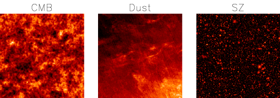
Figure 1: Spatial template of the CMB, dust and SZ components used in the simulations presented in the text. For visibility the SZ template is displayed in log scale.

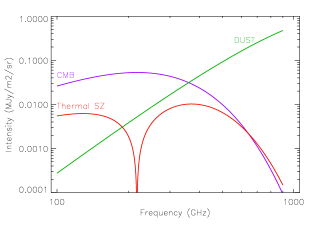
Figure 2: Electromagnetic spectrum of the CMB, dust and SZ components used in the simulations presented in the text. These spectra fully define the missing matrix $Ab$ when the beam smoothing effects are neglected.

From the modeling point of view, the CMB component is not special and therefore we can write

$$y_{\nu}(\nu,{\mathb{r}})=\sum_{i=1}^{N_{c}}g_{i}(\nu)\;s_{i}({\mathb{r}})*b_{\nu}({\mathb{r}})+n_{\nu}({\mathb{r}})$$

where $N_{c}=N_{f}+1$. Thus, for a set of detectors $d={1,..,N_{d}}$ operating at electromagnetic frequencies $\nu_{d}$

$$y_{d}({\mathb{r}})=\sum_{i=1}^{N_{c}}A_{di}\;s_{i}({\mathb{r}})*b_{d}({\mathb{r}})+n_{d}({\mathb{r}})$$ (2)

where $A_{di}=g_{i}(\nu_{d})$ is a $N_{d}\times N_{c}$ matrix called the mixing matrix.

If we assume the instrumental response of the detectors to be spatially invariant it is more convenient to work in Fourier space, since the convolution in equation 2 becomes a simple multiplication and we obtain

$$\tilde{y}_{d}({\mathb{k}})=\sum_{i=1}^{N_{c}}\tilde{A}_{di}({\mathb{k}})\;\tilde{s}_{i}({\mathb{k}})+\tilde{n}_{d}({\mathb{k}})$$ (3)

where $\tilde{A}_{di}({\mathb{k}})=A_{di}\tilde{b}_{d}({\mathb{k}})$. Further, equation 3 is verified for each Fourier mode ${\mathb{k}}$ independently and if the components are assumed to be stationary random variables then the separation can be performed also independently at each Fourier mode.

Hereafter, to simplify the mathematical formalism in the following sections, we will not include the beam smoothing in the analysis, so that equation 3 in matrix notation and for each mode ${\mathb{k}}$ becomes

$${\mathb{y}}({\mathb{k}})={\mathb{A}}\;{\mathb{s}}({\mathb{k}})+{\mathb{n}}({\mathb{k}})$$ (4)

where ${\mathb{y}}$, ${\mathb{s}}$ and ${\mathb{n}}$ are column vectors containing $N_{d}$, $N_{c}$ and $N_{d}$ complex components respectively, and the matrix ${\mathb{A}}$ has dimensions $N_{d}\times N_{c}$.

Note that the separation of components requires the joint estimation of the sources ${\mathb{s}}$ and the mixing matrix ${\mathb{A}}$ (or at least some of its elements). In practice, the noise covariance matrix, ${\mathb{R}}_{\epsilon}=E\left({\mathb{n}}{\mathb{n}}^{T}\right)$ is not very well known and in most cases has also to be estimated from the observed data, ${\mathb{y}}$.

3 Simulated Observations for the Planck High Frequency Instrument

The Planck satellite will measure the emission from the whole sky in the electromagnetic frequency range 30 to 850 GHz. The data will be taken using two independent instruments, the Low Frequency Instrument (LFI) and the High Frequency Instrument (HFI). Here, we only consider (as a starting point for devising and testing component separation methods) the HFI instrument which observes the sky in 6 frequency channels between 100 and 850 GHz. In the frequency range of the HFI instrument, the CMB radiation dominates at low frequencies and the dust emission at high frequencies. In addition, we expect significant contribution from the SZ effect in clusters of galaxies. The rest of the foreground components present weak emission at the HFI electromagnetic frequencies.

We simulate, following the model introduced in section 2, observations from 6 detectors ($N_{d}=6$) corresponding to the 6 HFI frequency channels. To reduce the computing time we restrict our simulations to small patches of the sky of $300\times 300$ square pixels of 2.5 arcmin as described in Delabrouille et al. (2001b). Working on small maps finds also a theoretical justification in the fact that the spectrum of emission of the dust (for instance) is known to vary slightly from a region of the sky to the other. The instrumental noise for each detector is considered white and Gaussian of zero mean and of rms expected for the HFI instrument channels. We also assume no correlation between the noise of the different detectors.

The simulations include 3 components ($N_{c}=3$), CMB radiation, dust emission and SZ effect in clusters of galaxies. The CMB component is a Gaussian randomly generated realisation of CMB anisotropies obtained from a theoretical spatial power spectrum calculated with CMBFAST Seljak and Zaldarriaga (2000). The electromagnetic frequency dependence of the CMB component is the derivative with respect to temperature of a Planck Blackbody spectrum, at temperature T=2.726 K. The dust component was obtained by extrapolation of the IRAS satellite 100 $\mu$m map (which serves as a spatial template) to the HFI frequencies, with an electromagnetic spectrum proportional to $\nu^{2}B_{\nu}(T=17.5\,{\rm K})$. Finally, the spatial template for the SZ component, due to the inverse-Compton scattering of primordial photons by hot electrons in the ionised gaz present in clusters of galaxies, was obtained from a simulation of the spatial distribution of the SZ comptonization parameter Delabrouille et al. (2001a). The emission law of the SZ emission is known theoretically, and depends only on the frequency of observation (in the Kompaneets approximation, which we assume here, see Birkinshaw (1999) for details).
The simulated observations are obtained from the superposition of the three above spatial templates with mixing coefficients set by the electromagnetic spectra of emission and the frequency of observation. The observations used as inputs in the separation procedure (with noise added at the level expected for Planck HFI detectors) are shown in figure 3.

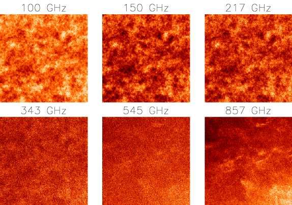
Figure 3: Simulated observations of the six HFI channels.

4 The separation method

The blind separation of sources constitutes a common example of missing data problem (problems for which only partial information is available) in the literature McLachlan and Krishnan (1996). Indeed, following equation 4 and considering the estimation of the mixing matrix, ${\mathb{A}}$, from a set of observations ${\mathb{y}}$, we can consider the components of the mixture, ${\mathb{s}}$ as the missing data in our problem because they are not directly available to the observer. As discussed in the previous sections, we are also interested in the estimation of the noise covariance matrix, ${\mathb{R}}$, which can be considered as an additional parameter in the separation.

Given the observations ${\mathb{y}}$, our approach is thus to estimate first the mixing matrix ${\mathb{A}}$ and the noise covariance matrix ${\mathb{R}}_{\epsilon}$ by maximizing the log-likelihood function $\log\,{\bf p}({\mathb{y}}_{1..K}\,|\,{\mathb{A}},\,{\mathb{R}}_{\epsilon})$,

$$(\widehat{{\mathb{A}}},\,\widehat{{\mathb{R}}}_{\epsilon})=\mathop{\mathrm{arg\,max}}_{{\mathb{A}},\,{\mathb{R}}_{\epsilon}}\;{\log\,{\bf p}({\mathb{y}}_{1..K}\,|\,{\mathb{A}},\,{\mathb{R}}_{\epsilon})}$$

The maximization of this log-likelihood will be made with a specific implementation of the Expectation Maximization (EM) algorithm introduced by Dempster-Laird-Rubin in Dempster et al. (1977). The estimation of the source templates is done afterwards by inverting the linear system $y=As+n$ using a classical inversion method as done by Bouchet and Gispert in Bouchet and Gispert (1999).

4.1 The EM algorithm: formalism

Let’s consider a missing data problem with observed data $({\mathb{y}}(k))_{k\in\{1..K\}}$ and missing data $({\mathb{x}}(k))_{k\in\{1..K\}}$, for which we want to estimate the set of parameters, ${\boldsymbol{\theta}}$. Hereafter, we will note as the incomplete-data problem that for which only the observed data are used to obtain the unknown parameters, and the complete-data problem, that for which the missing data are also considered in the solution.

An optimal estimate of ${\boldsymbol{\theta}}$, $\hat{{\boldsymbol{\theta}}}$ can be obtained by maximizing its incomplete log-likelihood function,

$$\mathcal{L}({\boldsymbol{\theta}})=\log{\bf p}({\mathb{y}}\,|\,{\boldsymbol{\theta}})$$

However, in many practical cases, this function is complex and difficult to work with and it is more convenient to solve the complete-data problem.

The EM algorithm permits to solve the incomplete data problem. It is an iterative algorithm which generates a sequence of approximations to find the maximum observed likelihood estimator when only partial information is available, by marginalizing at each iteration over the missing data.

At iteration $j+1$ of the algorithm we can write

$${\boldsymbol{\theta}}^{j+1}={\mathcal{M}}({\boldsymbol{\theta}}^{j})$$ (5)

where ${\mathcal{M}}$ is a mapping function, named the re-estimation transformation. After the initialization to an arbitrary point ${\boldsymbol{\theta}}^{0}\in{\boldsymbol{\Theta}}$, the new estimate of ${\boldsymbol{\theta}}$ is computed using equation (5), until a fixed point is obtained such that ${\boldsymbol{\theta}}^{j+1}={\boldsymbol{\theta}}^{j}$. The mapping ${\mathcal{M}}$ is performed in two steps

• ${\mathrm{E}}\,$-step: Computation of $Q({\boldsymbol{\theta}},{\boldsymbol{\theta}}^{j})={\mathrm{E}}\,\;\left[\log{{\bf p}({\mathb{y}},{\mathb{x}}\,|\,{\boldsymbol{\theta}})}\,|\,{\mathb{y}},{\boldsymbol{\theta}}^{j}\right]$

• M-step: Find ${\boldsymbol{\theta}}^{j+1}=\displaystyle{\mathop{\mathrm{arg\,max}}_{{\boldsymbol{\theta}}\in{\boldsymbol{\Theta}}}\;{Q({\boldsymbol{\theta}},{\boldsymbol{\theta}}^{j})}}$

where ${\bf p}({\mathb{y}}\,|\,{\boldsymbol{\theta}})$ and ${\bf p}({\mathb{y}},{\mathb{x}}\,|\,{\boldsymbol{\theta}})$ denote the incomplete and the complete probability distributions respectively.

A fundamental property of the EM algorithm is the fact that it ensures the monotonous increasing of the incomplete likelihood function. Any value of ${\boldsymbol{\theta}}$ such that $Q({\boldsymbol{\theta}},{\boldsymbol{\theta}}^{j})\geq Q({\boldsymbol{\theta}}^{j},{\boldsymbol{\theta}}^{j})$ increases as well the incomplete log-likelihood, $i.e$, $\mathcal{L}({\boldsymbol{\theta}})\geq\mathcal{L}_{i}({\boldsymbol{\theta}}^{j})$. Moreover, $\hat{{\boldsymbol{\theta}}}$ is a critical point of the incomplete likelihood ${\bf p}({\mathb{y}}\,|\,{\boldsymbol{\theta}})$ if and only if it is a fixed point of the re-estimation transformation, ${\mathcal{M}}$. A more detailed description of the convergence properties of the EM algorithm can be found in Dempster et al. (1977).

Basic steps in the EM algorithm

The implementation of the EM algorithm starts by choosing an initial guess for the unknown parameters, ${\boldsymbol{\theta}}^{0}$, which is used in the first iteration of the algorithm. Then, at each iteration $j+1$ the following basic steps are performed

• i) ${\boldsymbol{\theta}}=\widehat{{\boldsymbol{\theta}}}^{j}$.

• ii) ${\mathrm{E}}\,$-step: Compute $Q({\boldsymbol{\theta}}^{\prime},{\boldsymbol{\theta}})$.

• iii) M-step: Find ${\boldsymbol{\theta}}^{j+1}$ such that $Q({\boldsymbol{\theta}}^{j+1},{\boldsymbol{\theta}})\geq Q({\boldsymbol{\theta}}^{\prime},{\boldsymbol{\theta}})$ for all ${\boldsymbol{\theta}}^{\prime}\in{\boldsymbol{\Theta}}$.

The iterative procedure is stopped when a fixed point is reached so that ${\boldsymbol{\theta}}^{j+1}={\boldsymbol{\theta}}^{j+1}$.

Penalized EM algorithm

In a Bayesian framework, we can consider the parameters ${\boldsymbol{\theta}}$ as random variables distributed according to an a priori ${\bf p}({\boldsymbol{\theta}}\,|\,\xi)$. The a posteriori distribution for ${\boldsymbol{\theta}}$, ${\bf p}({\boldsymbol{\theta}}\,|\,{\mathb{y}},\,\xi)$ can be considered as a penalized version of the likelihood ${\bf p}({\mathb{y}}\,|\,{\boldsymbol{\theta}})$ such that:

$${\bf p}({\boldsymbol{\theta}}\,|\,{\mathb{y}},\,\xi)\propto{\bf p}({\mathb{y}}\,|\,{\boldsymbol{\theta}})\,{\bf p}({\boldsymbol{\theta}}\,|\,\xi)$$

The EM algorithm can be extended to a penalized version that converges to a local maximum of the penalized version of the likelihood function Hero and Fessler (1985). The penalized version of the EM functional $Q_{p}({\boldsymbol{\theta}},{\boldsymbol{\theta}}^{k})$ is given by:

$$\begin{array}[]{lll}Q_{p}({\boldsymbol{\theta}},{\boldsymbol{\theta}}^{j})&=&{\mathrm{E}}\bigl{[}\log{{\bf p}({\mathb{y}},{\mathb{x}},\,{\boldsymbol{\theta}}\,|\,\xi)}\,|\,{\mathb{y}},{\boldsymbol{\theta}}^{j}\bigr{]}\\ {}&=&{\mathrm{E}}\bigl{[}\log{{\bf p}({\mathb{y}},{\mathb{x}}\,|\,{\boldsymbol{\theta}})}\,|\,{\mathb{y}},{\boldsymbol{\theta}}^{j}\bigr{]}+\log{{\bf p}({\boldsymbol{\theta}}\,|\,\xi)}\\ {}&=&Q_{ML}({\boldsymbol{\theta}},{\boldsymbol{\theta}}^{j})+\log{{\bf p}({\boldsymbol{\theta}}\,|\,\xi)}\end{array}$$

4.2 Application of the EM-algorithm to source separation

Missing information model

Now we consider the application of the EM algorithm to the problem of source separation in Fourier space. For this reason, we call it Spectral EM algorithm.

As discussed in section $2$, at each mode ${\mathb{k}}$, the vector of observations ${\mathb{y}}$ arises from the following model

$${\mathb{y}}({\mathb{k}})={\mathb{A}}\,{\mathb{s}}({\mathb{k}})+{\mathb{n}}({\mathb{k}})$$

Matrix ${\mathb{A}}$ is the unknown (or partially unknown) mixing matrix and we assume that ${\mathb{n}}({\mathb{k}})$ is a zero mean Gaussian white noise with unknown diagonal covariance matrix ${\mathb{R}}_{\epsilon}$. We will consider ${\boldsymbol{\theta}}=({\mathb{A}},{\mathb{R}}_{\epsilon})$ the unknown parameters to be estimated.

The incomplete likelihood function we want to maximize, ${\bf p}({\mathb{y}}_{1..K}\,|\,{\mathb{A}},\,{\mathb{R}}_{\epsilon})$, can be derived by marginalizing the joint distribution ${\bf p}({\mathb{y}}_{1..K},\,{\mathb{s}}_{1..K}\,|\,{\mathb{A}},\,{\mathb{R}}_{\epsilon})$ over sources as follows:

$${\bf p}({\mathb{y}}_{1..K}\,|\,{\mathb{A}},\,{\mathb{R}}_{\epsilon})=\int_{{\mathb{s}}_{1..K}}{\bf p}({\mathb{y}}_{1..K},\,{\mathb{s}}_{1..K}\,|\,{\mathb{A}},\,{\mathb{R}}_{\epsilon})\,d\,{\mathb{s}}_{1..K}$$

In our method, we assume a prior knowledge of the sources spatial power spectra, i.e. the components ${\mathb{s}}({\mathb{k}})$ are assumed to follow an a priori probability distribution of the form

$${\bf p}({\mathb{s}}({\mathb{k}})\,|\,{\mathb{C}}({\mathb{k}}))$$

where $({\mathb{C}}_{k})_{k\in{\mathb{I}}}$ represent the a priori spatial power spectrum shape.

Assuming stationarity for the sources, the Fourier modes are not correlated and we can perform the separation at each Fourier mode independently. The independence in the spectral domain can be written as:

$$\left\{\begin{array}[]{lll}{\bf p}\left(\,\,({\mathb{s}}({\mathb{k}}))_{{\mathb{k}}\in{\mathb{I}}}\,\,|\,\,({\mathb{C}}({\mathb{k}}))_{{\mathb{k}}\in{\mathb{I}}}\,\,\right)=\displaystyle{\prod_{{\mathb{k}}\in{\mathb{I}}}{\bf p}({\mathb{s}}({\mathb{k}})\,|\,{\mathb{C}}({\mathb{k}}))}\\ {}\\ {\bf p}\left(\,\,({\mathb{n}}({\mathb{k}}))_{{\mathb{k}}\in{\mathb{I}}}\,\,|\,\,{\mathb{R}}_{\epsilon}\,\,\right)=\displaystyle{\prod_{{\mathb{k}}\in{\mathb{I}}}{{\bf p}({\mathb{n}}({\mathb{k}})\,|\,{\mathb{R}}_{\epsilon})}}\\ \end{array}\right.$$

Because of this independence, ${\mathb{k}}$ is replaced by the integer index $k$ and ${\mathb{I}}=\{1..K\}$ is a fixed arbitrary arrangement, where $K$ is the number of Fourier modes.

We can write the complete data $({\mathb{y}}_{1..K},\,{\mathb{s}}_{1..K})$ probability distribution as

$${\bf p}({\mathb{y}}_{1..K},\,{\mathb{s}}_{1..K}\,|\,{\mathb{A}},\,{\mathb{R}}_{\epsilon})=\displaystyle{\prod_{k=1}^{K}}{\bf p}({\mathb{y}}_{k}\,|\,{\mathb{s}}_{k}\,{\mathb{A}},\,{\mathb{R}}_{\epsilon})\,\displaystyle{\prod_{k=1}^{K}}{\bf p}({\mathb{s}}_{k}\,|\,{\mathb{C}}_{k})$$

so that, the complete log-likelihood function $\mathcal{L}_{c}$ is given by

$$\begin{array}[]{lll}\mathcal{L}_{c}({\mathb{A}},\,{\mathb{R}}_{\epsilon})&=&{\bf\log}\,{\bf p}({\mathb{y}}_{1..K},\,{\mathb{s}}_{1..K}\,|\,{\mathb{A}},\,{\mathb{R}}_{\epsilon})\\ {}\\ {}&=&\displaystyle{\sum_{k=1}^{K}}{\bf\log}\,{\bf p}({\mathb{y}}_{k}\,|\,{\mathb{s}}_{k}\,{\mathb{A}},\,{\mathb{R}}_{\epsilon})\,+\,\displaystyle{\sum_{k=1}^{K}}{\bf\log}\,{\bf p}({\mathb{s}}_{k}\,|\,{\mathb{C}}_{k})\\ {}\\ {}&=&\displaystyle{\sum_{k=1}^{K}}\left(-\frac{1}{2}\,|\,2\,\pi\,{\mathb{R}}_{\epsilon}\,|-\frac{1}{2}({\mathb{y}}_{k}-{\mathb{A}}\,{\mathb{s}}_{k})^{T}{\mathb{R}}_{\epsilon}^{-1}\,({\mathb{y}}_{k}-{\mathb{A}}\,{\mathb{s}}_{k})\right)+cst\end{array}$$ (6)

Implementation of the Spectral EM algorithm

The functional $Q({\boldsymbol{\theta}},\,{\boldsymbol{\theta}}^{k})$ is given by

$$\begin{array}[]{lll}Q\left({\boldsymbol{\theta}}\,|\,{\boldsymbol{\theta}}^{j}\right)&=&{\mathrm{E}}\,_{{\mathb{s}}\,|\,{\boldsymbol{\theta}}^{j}}\left[\log\,p({\mathb{y}}_{1..K},\,{\mathb{s}}_{1..K}\,|\,{\boldsymbol{\theta}})\,|\,{\mathb{y}}_{1..K},\,{\boldsymbol{\theta}}^{j}\right]\\ {}\\ {}&=&\int_{{\mathb{s}}_{1..K}}\log\,p({\mathb{y}}_{1..K},\,{\mathb{s}}_{1..K}\,|\,{\boldsymbol{\theta}})\,p({\mathb{s}}_{1..K}\,|\,{\mathb{y}}_{1..K},\,{\boldsymbol{\theta}}^{j})\,d\,{\mathb{s}}_{1..K}\par\end{array}$$

and using equation 6, we get,

$$Q\left({\boldsymbol{\theta}}\,|\,{\boldsymbol{\theta}}^{j}\right)=-\frac{K}{2}\log{2\pi{\mathb{R}}_{\epsilon}}-\frac{K}{2}\mbox{Tr}\left({\mathb{R}}_{\epsilon}^{-1}(\widehat{{\mathb{R}}}_{yy}-{\mathb{A}}\widehat{{\mathb{R}}}_{ys}^{T}-\widehat{{\mathb{R}}}_{ys}{\mathb{A}}^{T}+{\mathb{A}}\widehat{{\mathb{R}}}_{ss}{\mathb{A}}^{T})\right)+cst$$

where

$$\left\{\begin{array}[]{lll}\widehat{{\mathb{R}}}_{yy}&=&\frac{1}{K}\sum_{k}{\mathb{y}}_{k}{\mathb{y}}_{k}^{T}\\ \widehat{{\mathb{R}}}_{ys}&=&\frac{1}{K}\sum_{k}{\mathb{y}}_{k}{\mathrm{E}}\,\,\left[{\mathb{s}}_{k}^{T}\,|\,{\mathb{y}}_{k},{\boldsymbol{\theta}}^{j}\right]\\ \widehat{{\mathb{R}}}_{ss}&=&\frac{1}{K}\sum_{k}{\mathrm{E}}\,\,\left[{\mathb{s}}_{k}{\mathb{s}}_{k}^{T}\,|\,{\mathb{y}}_{k},{\boldsymbol{\theta}}^{j}\right]\end{array}\right.$$ (7)

To obtain the parameter ${\boldsymbol{\theta}}^{j+1}=({\mathb{A}}^{j+1},{\mathb{R}}_{\epsilon}^{j+1})$ at iteration $j+1$, we solve the following gradient equations with respect to ${\mathb{A}}$ and ${\mathb{R}}_{\epsilon}$ in order to maximize the functional $Q$. The complete log-likelihood function $\mathcal{L}_{c}$ of equation 6 is quadratic as a function of ${\mathb{A}}$ and consequently, the functional $Q({\mathb{A}},\,{\mathb{R}}_{\epsilon}\,|\,{\mathb{A}}^{j},\,{\mathb{R}}_{\epsilon}^{j})$ is also quadratic in ${\mathb{A}}$ and its derivative with respect to ${\mathb{R}}_{\epsilon}$ can be easily calculated. Therefore, $\widehat{{\mathb{A}}}^{j+1}$ and $\widehat{{\mathb{R}}_{\epsilon}}^{j+1}$ are easily derived.

$$\left\{\begin{array}[]{l}\frac{\partial{Q}}{\partial{{\mathb{A}}}}=K{\mathb{R}}_{\epsilon}^{-1}(\widehat{{\mathb{R}}}_{ys}-{\mathb{A}}\widehat{{\mathb{R}}}_{ss})=0\\ {}\\ \frac{\partial{Q}}{\partial{{\mathb{R}}_{\epsilon}}}=\frac{K}{2}{\mathb{R}}_{\epsilon}^{-1}(\widehat{{\mathb{R}}}_{yy}-{\mathb{A}}\widehat{{\mathb{R}}}_{ys}^{T}-\widehat{{\mathb{R}}}_{ys}{\mathb{A}}^{T}+{\mathb{A}}\widehat{{\mathb{R}}}_{ss}{\mathb{A}}^{T}){\mathb{R}}_{\epsilon}^{-1}-\frac{K}{2}{\mathb{R}}_{\epsilon}^{-1}=0\end{array}\right.$$ (8)

which yields to the re-estimation equations

$$\left\{\begin{array}[]{ll}{\mathb{A}}^{j+1}=\widehat{{\mathb{R}}}_{ys}\,(\widehat{{\mathb{R}}}_{ss})^{-1}\\ {}\\ {\mathb{R}}_{\epsilon}^{j+1}=\widehat{{\mathb{R}}}_{yy}-{\mathb{A}}^{j+1}\widehat{{\mathb{R}}}_{ys}^{T}-\widehat{{\mathb{R}}}_{ys}({\mathb{A}}^{j+1})^{T}+{\mathb{A}}^{j+1}\widehat{{\mathb{R}}}_{ss}({\mathb{A}}^{j+1})^{T}\end{array}\right.$$ (9)

We now focus on the computation of the statistics (7) involved in the re-estimation transformation (9). The statistic $\widehat{{\mathb{R}}}_{yy}$, which represents the auto-covariance of the observations, is directly computed from the data ${\mathb{y}}_{1..K}$, and remains constant throughout iterations of the EM algorithm. The statistic $\widehat{{\mathb{R}}}_{ys}$ represents the a posteriori cross-covariance of the observations and the sources and the statistic $\widehat{{\mathb{R}}}_{ss}$ represents the a posteriori auto-covariance of the sources. The statistics $\widehat{{\mathb{R}}}_{ys}$ and $\widehat{{\mathb{R}}}_{ss}$ need, respectively, the computation of the a posteriori expectation ${\mathrm{E}}\,\left[{\mathb{s}}_{k}\,|\,{\mathb{y}}_{k},\,{\boldsymbol{\theta}}^{j}\right]$ and the a posteriori covariance ${\mathrm{E}}\,\left[{\mathb{s}}_{k}\,{\mathb{s}}_{k}^{T}\,|\,{\mathb{y}}_{k},\,{\boldsymbol{\theta}}^{j}\right]$ which depends on the a priori distribution of the sources ${\bf p}({\mathb{s}}({\mathb{k}})\,|\,{\mathb{C}}({\mathb{k}}))$. We consider in the following two different prior distributions:

(i) Gaussian prior which corresponds to the Wiener filtering
(ii) Entropic prior which corresponds to the MEM deconvolution.


Gaussian prior:

The a priori distribution of the source vector ${\mathb{s}}_{k}$ is assumed to be a zero mean Gaussian with covariance ${\mathb{C}}_{k}$:

$${\bf p}({\mathb{s}}_{k}\,|\,{\mathb{C}}_{k})\propto\exp\left[-\frac{1}{2}{\mathb{s}}_{k}^{T}{\mathb{C}}_{k}^{-1}{\mathb{s}}_{k}\right]$$

Then, the a posteriori distribution is

$$p({\mathb{s}}_{k}|{\mathb{y}}_{k},{\mathb{A}},{\mathb{R}}_{\epsilon})\propto\exp\left[-\Phi({\mathb{s}}_{k})\right]$$

with

$$\Phi({\mathb{s}}_{k})=\frac{1}{2}({\mathb{y}}_{k}-{\mathb{A}}{\mathb{s}}_{k})^{T}{\mathb{R}}_{\epsilon}^{-1}({\mathb{y}}_{k}-{\mathb{A}}{\mathb{s}}_{k})+\frac{1}{2}{\mathb{s}}_{k}^{T}{\mathb{C}}_{k}^{-1}{\mathb{s}}_{k}$$

Thus, the expectations are easily derived as follows

$$\left\{\begin{array}[]{ccccc}{\mathrm{E}}\,[{\mathb{s}}_{k}]={\mathb{e}}_{k}=\left[{\mathb{A}}^{T}{\mathb{R}}_{\epsilon}^{-1}{\mathb{A}}+{\mathb{C}}_{k}^{-1}\right]^{-1}{\mathb{A}}^{T}{\mathb{R}}_{\epsilon}^{-1}{\mathb{y}}_{k}\\ {}\hfil\\ {\mathrm{E}}\,[{\mathb{s}}_{k}{\mathb{s}}_{k}^{t}]=\left[{\mathb{A}}^{T}{\mathb{R}}_{\epsilon}^{-1}{\mathb{A}}+{\mathb{C}}_{k}^{-1}\right]^{-1}+{\mathb{e}}_{k}{\mathb{e}}_{k}^{T}\end{array}\right.$$

Entropic prior:

For most foreground components the Gaussian prior does not fully represent the underlying physical processes. For this reason, Hobson et al. Hobson et al. (1998) introduced an entropic prior for the sources. Defining ${\mathb{h}}_{k}$ a hidden vector such that ${\mathb{s}}_{k}={\mathb{L}}_{k}{\mathb{h}}_{k}$, where ${\mathb{L}}_{k}$ is obtained from the Cholesky decomposition of the spectrum of sources ${\mathb{C}}_{k}$, the entropic prior can be expressed as follows

$$p({\mathb{h}}_{k}\,|\,{\mathb{m}}_{k},\,\alpha)\propto\exp\left[\alpha{\mathcal{S}}({\mathb{h}}_{k},{\mathb{m}}_{k})\right]$$

where ${\mathcal{S}}({\mathb{h}}_{k},{\mathb{m}}_{k})$ is the complex cross-entropy of ${\mathb{h}}_{k}$ and ${\mathb{m}}_{k}$ is a default model for ${\mathb{h}}_{k}$

$$\left\{\begin{array}[]{lll}{\mathcal{S}}({\mathb{h}}_{k},{\mathb{m}}_{k})=\sum_{j=1}^{n}\left[\psi_{kj}-2m_{kj}-h_{kj}\log{\frac{\psi_{kj}+h_{kj}}{2m_{kj}}}\right]\\ {}\\ \psi_{kj}=\sqrt{h_{kj}^{2}+4m_{kj}^{2}}\\ {}\\ {\mathb{m}}_{k}=\left(\begin{array}[]{l}1\\ \vdots\\ 1\end{array}\right)\par\end{array}\right.$$

Then, the a posteriori distribution of ${\mathb{h}}_{k}$ is:

$$p({\mathb{h}}_{k}|{\mathb{y}}_{k},{\mathb{A}},{\mathb{R}}_{\epsilon})\propto\exp\left[-\Phi({\mathb{h}}_{k})\right]$$

with

$$\Phi({\mathb{h}}_{k})=\frac{1}{2}({\mathb{y}}_{k}-{\mathb{A}}{\mathb{L}}{\mathb{h}}_{k})^{T}{\mathb{R}}_{\epsilon}^{-1}({\mathb{y}}_{k}-{\mathb{A}}{\mathb{L}}{\mathb{h}}_{k})-\alpha{\mathcal{S}}({\mathb{h}}_{k},{\mathb{m}}_{k})$$

The function $\Phi({\mathb{h}}_{k})$ being convex, the a posteriori expectation of ${\mathb{h}}_{k}$ can be approximated by the minimum $\widehat{{\mathb{h}}}_{k}$ of this function and the covariance by the inverse of the Hessian $[{\mathb{H}}(\widehat{{\mathb{h}}}_{k})]^{-1}$ computed at this minimum:

$$\left\{\begin{array}[]{l}{\mathrm{E}}\,[{\mathb{s}}_{k}]={\mathb{L}}\widehat{{\mathb{h}}}_{k}\\ {}\\ {\mathrm{E}}\,[{\mathb{s}}_{k}{\mathb{s}}_{k}^{T}]={\mathb{L}}[{\mathb{H}}(\widehat{{\mathb{h}}}_{k})]^{-1}{\mathb{L}}^{T}+{\mathrm{E}}\,[{\mathb{s}}_{k}]{\mathrm{E}}\,[{\mathb{s}}_{k}]^{*}\end{array}\right.$$

The minimum $\widehat{{\mathb{h}}}_{k}$ can be computed with an iterative minimization algorithm. Expressions for the gradient and the hessian of $\Phi$ are easily derived,

$$\left\{\begin{array}[]{l}\nabla_{{\mathb{h}}_{k}}\Phi={\mathb{L}}^{T}{\mathb{A}}^{T}{\mathb{R}}_{\epsilon}^{-1}({\mathb{A}}{\mathb{L}}{\mathb{h}}_{k}-{\mathb{y}}_{k})+\alpha\,\left[\log{\left(\frac{\psi_{kj}+h_{k}j}{2mu_{j}}\right)}\right]_{j=1..n}\\ {}\\ \nabla^{2}_{{\mathb{h}}_{k}}\Phi={\mathb{L}}^{T}{\mathb{A}}^{T}{\mathb{R}}_{\epsilon}^{-1}{\mathb{A}}{\mathb{L}}+\alpha\,{\bf diag}\left[2m_{k}j/\psi_{kj}\right]\end{array}\right.$$

5 Application to Planck HFI simulated observations

5.1 Prior information

The penalized form of the spectral EM algorithm permits to naturally include a priori information about the parameters we want to estimate. In the case of CMB observations, one will naturally dispose of additional information from theoretical predictions or from previous observations at the same or other electromagnetic frequencies (although in most cases at lower resolution). We can take those into account in the separation procedure. In particular, the electromagnetic spectrum of the anisotropies of the CMB radiation is accurately known at centimetre and millimetre wavelengths, and therefore there is no need to estimate it. Further, the emission from dust grains has also been measured by the IRAS satellite at 100 $\mu$m providing a first class template of it.

For a first test of the convergence capabilities of the algorithm we have only considered weak a priori information about the spatial spectrum of the components. For the CMB component, the a priori spatial power spectrum was taken to be the theoretical model fitting best current observations Delabrouille et al. (2001b) and for dust, the mean spatial spectrum measured by the IRAS satellite at 100$\mu$m Schlegel et al. (1998). A circular spatial spectrum was assumed as a prior for the SZ component. This spectrum was obtained from an empirical fit to numerical simulations of SZ templates Delabrouille et al. (2001a). No prior information was assumed for the electromagnetic spectrum of the components, i.e., no prior on the mixing matrix.

5.2 Results

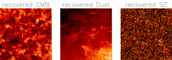
Figure 4: Recovered spatial template of the CMB, dust and SZ components. For visibility, the recovered SZ is displayed in log scale.

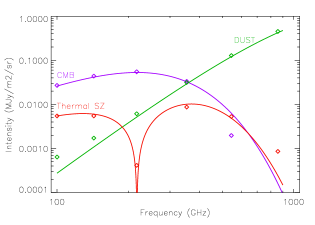
Figure 5: The figure shows the recovered electromagnetic spectrum of the components (diamonds) overplotted to the input spectrum (solid lines).

The spectral EM algorithm has been applied to the simulated HFI observations presented in section 3. The prior information on the spatial spectra of the components is used for a Wiener filtering estimation of the missing data at each iteration of the algorithm. The algorithm has been implemented in C and needs about 20000 iterations to attain complete separation running on a 1GHz PENTIUM IV PC, for a total running time of about 8 hours of CPU time on $300\times 300$ pixels maps.

The recovered spatial distributions of the components are shown in figure 4. CMB and dust components are recovered satisfactorily, with signal to noise ratio of about 5, better than the signal to noise ratio in any of the detectors. The SZ is recovered with signal to noise of 1, not very satisfactorily (although the brightest clusters can be picked by eye on the output). This is essentially due to its peaky structure for which a Fourier treatment with very limited spectral a priori information is not very appropriate.

The recovered electromagnetic spectra are shown in figure 5. The CMB and dust spectra are recovered to better than 1% for all detectors where the level of the components is not negligible. The recovered electromagnetic spectrum of the SZ emission was multiplied by a global calibration factor due to a mismatch between the assumed power spectrum and the true (empirical) one. In this way the true spectrum is recovered to better than 10% for those channels with significant SZ contribution.

6 Conclusions

The spectral version of the EM algorithm presented in this paper constitutes a useful tool for the semi-blind separation of astrophysical components in noisy mixtures and in particular to separate CMB and foreground components in future space observations of the CMB. A first test of the algorithm on simulated Planck HFI observations with 3 components, CMB, dust and SZ emissions, has been proven successful. We have been able to achieve complete separation with signal to noise of 5 and also to recover the electromagnetic spectrum of the components to better than 1 % in about 20.000 iterations.

In the present analysis we do not consider the smearing out of the observations due to the finite resolution of the detectors. However, the spectral EM algorithm can be easily modified as proposed in section 2 to account for this. A modified version of algorithm is already under testing and will permit the separation of multi-frequency observations at different resolutions.

Further development of the algorithm is in progress including better use of the available prior information. In real experiments, one would like to take advantage of the fact that the electromagnetic spectrum is known for some of the components in which case there is no need to estimate it within the separation algorithm. The EM algorithm as presented here can naturally account for this fact by either reducing the number of free parameters to estimate or including a penalization term when only partial information is available. A first version of the algorithm implementing the former is already available and produces good preliminary results.

The major drawback of our present implementation of the spectral EM algorithm is the computation time needed for convergence (about 20000 iterations and 8 hours of CPU to converge to complete separation). The acceleration of the algorithm is needed before it can be applied to full sky data sets or tested statistically by Monte-Carlo methods. Acceleration techniques are currently being explored.

References

- Baccigalupi et al. [2000] C. Baccigalupi, L. Bedini, C. Burigana, G. De Zotti, A. Farusi, D. Maino, M. Maris, F. Perrotta, E. Salerno, L. Toffolatti, and A. Tonazzini. MNRAS, 318:769–780, Nov. 2000.
- Birkinshaw [1999] M. Birkinshaw. Physics Reports, 310:97–195, 1999.
- Bouchet and Gispert [1999] F. R. Bouchet and R. Gispert. New Astronomy, 4:443–479, Nov. 1999.
- de Bernardis et al. [2000] P. de Bernardis, P. A. R. Ade, J. J. Bock, J. R. Bond, J. Borrill, A. Boscaleri, K. Coble, B. P. Crill, G. De Gasperis, P. C. Farese, P. G. Ferreira, K. Ganga, M. Giacometti, E. Hivon, V. V. Hristov, A. Iacoangeli, A. H. Jaffe, A. E. Lange, L. Martinis, S. Masi, P. V. Mason, P. D. Mauskopf, A. Melchiorri, L. Miglio, T. Montroy, C. B. Netterfield, E. Pascale, F. Piacentini, D. Pogosyan, S. Prunet, S. Rao, G. Romeo, J. E. Ruhl, F. Scaramuzzi, D. Sforna, and N. Vittorio. Nat., 404:955–959, Apr. 2000.
- De Zotti et al. [1999] G. De Zotti, L. Toffolatti, F. Argüeso, R. D. Davies, P. Mazzotta, R. B. Partridge, G. F. Smoot, and N. Vittorio. In AIP Conf. Proc. 476: 3K cosmology, page 204, 1999.
- Delabrouille et al. [2001a] J. Delabrouille, J. Melin, and M. Bartlett. In to appear in AMIBA 2001, High-z clusters, Missing Baryons and CMB polarization, ASP conf. series, L-W Chen, C-P Ma, K-W Ng and U-L Pen, eds., 2001a.
- Delabrouille et al. [2001b] J. Delabrouille, G. Patanchon, and E. Audit. To appear in MNRAS, 2001b.
- Dempster et al. [1977] A. Dempster, N. Laird, and D. Rubin. Journal of the Royal Statistical Society B, 39:1–38, 1977.
- Hanany et al. [2000] S. Hanany, P. Ade, A. Balbi, J. Bock, J. Borrill, A. Boscaleri, P. de Bernardis, P. G. Ferreira, V. V. Hristov, A. H. Jaffe, A. E. Lange, A. T. Lee, P. D. Mauskopf, C. B. Netterfield, S. Oh, E. Pascale, B. Rabii, P. L. Richards, G. F. Smoot, R. Stompor, C. D. Winant, and J. H. P. Wu. ApJ, 545:L5–L9, Dec. 2000.
- Hero and Fessler [1985] A. Hero and J. Fessler. Preprints, Dept. of Electrical Engineering and computer Science, University of Michigan,85-T-21, 1985.
- Hobson et al. [1998] M. P. Hobson, A. W. Jones, A. N. Lasenby, and F. R. Bouchet. MNRAS, 300:1–29, Oct. 1998.
- Hu and Sugiyama [1996] W. Hu and N. Sugiyama. ApJ, 471:542+, Nov. 1996.
- Jungman et al. [1996] G. Jungman, M. Kamionkowski, A. Kosowsky, and D. N. Spergel. Physical Review Letters, 76:1007–1010, Feb. 1996.
- McLachlan and Krishnan [1996] G. McLachlan and T. Krishnan. The EM algorithm and Extensions. Wiley Inter-Science, 1996.
- Schlegel et al. [1998] D. J. Schlegel, D. P. Finkbeiner, and M. Davis. ApJ, 500:525, June 1998.
- Seljak and Zaldarriaga [2000] U. Seljak and M. Zaldarriaga. ApJ. Suppl. ser., 129:431, 2000.
- Tegmark and Estathiou [1996] M. Tegmark and G. Estathiou. MNRAS, 281:1297, 1996.