Modified Newtonian Dynamics of Large Scale Structure

Abstract

We examine the implications of Modified Newtonian Dynamics (MOND) on the large scale structure in a Friedmann-Robertson-Walker universe. We employ a “Jeans swindle” to write a MOND-type relationship between the fluctuations in the density and the gravitational force, ${\bf g}$. In linear Newtonian theory, $|{\bf g}|$ decreases with time and eventually becomes $<\;g_{{}_{0}}$, the threshold below which MOND is dominant. If the Newtonian initial density field has a power-law power-spectrum of index $n<-1$, then MOND domination proceeds from small to large scale. At early times MOND tends to drive the density power-spectrum towards $k^{-1}$, independent of its shape in the Newtonian regime. We use N-body simulations to solve the MOND equations of motion starting from initial conditions with a CDM power-spectrum. MOND with the standard value $g_{{}_{0}}=10^{-8}{\mathrm{c}m\;s^{-2}}$, yields a high clustering amplitude that can match the observed galaxy distribution only with strong (anti-) biasing. A value of $g_{{}_{0}}\approx 10^{-9}{\mathrm{c}m\;s^{-2}}$, however, gives results similar to Newtonian dynamics and can be consistent with the observed large scale structure.

1 introduction

Perhaps the best evidence for the existence of dark matter is the flattening of rotation curves of many spiral galaxies. Newton’s $g_{{}_{N}}\sim 1/({\rm distance})^{2}$ law for the force of gravity predicts that the observed distribution of baryonic matter should show a fall off in the rotation curves, and hence the need for dark matter to explain the flattening. A universe predominantly filled with cold dark matter (CDM) is consistent with observations of the cosmic microwave background, and the galaxy population. Nevertheless, the dark matter scenario does not readily explain the shape of rotation curves of some galaxies in the inner regions (e.g., Moore 1994, Flores & Primack 1994, de Blok et al. 2001), the dark matter particle has not been discovered, and we lack a direct experimental verification of Newton’s law of gravity at low accelerations. So it seems prudent to examine alternative scenarios explaining the flattening of rotation curves. Modified Newtonian Dynamics (MOND) acting at low accelerations (e.g., Milgrom 1983, Bekenstein & Milgrom 1984) can explain the flattening of rotation curves without the need for dark matter. Two main versions of MOND exist. The first replaces Newton’s law of gravity at $g_{{}_{N}}<g_{{}_{0}}$ by $g\sim\sqrt{g_{{}_{0}}g_{{}_{N}}}$ where $g_{{}_{0}}\approx 1.2\times 10^{-8}{\mathrm{c}m\;s^{-2}}$ is found to give the best results in fitting the rotation curves. The second modifies the law of inertia at low accelerations. Here we adopt the first version where the equations of motion can be derived from a Lagrangian, admitting conservation of energy and momentum (Bekenstein & Milgrom 1984). Because of the success of MOND at fitting the rotation curves (e.g., Milgrom & Braun 1988, Begeman et al. 1991, Sanders 1996, de Blok & McGaugh 1998, Sanders & Verheijen 1998), it is worthwhile to push it further and confront it with observations of the large scale structure in the Universe (Felten 1984, McGaugh 1999, Sanders 2001). A problem here arises however. MOND, when applied to a uniform background, predicts the collapse of any finite region in the universe regardless of the mean density in that region (e.g., Felten 1984, Sanders 1998). To solve this problem Sanders (2001) proposed a two-field Lagrangian based theory of MOND in which the Friedmann-Robertson-Walker (FRW) background cosmology remains intact in the absence of fluctuations. He argued that this theory leads to large scale structure resembling Newtonian dynamics with CDM-like initial conditions. Here we take a simpler approach in which we employ the Jeans swindle to write a MOND type relationship between the fluctuations in the density and the gravitational force field. Although our procedure can be derived from a Lagrangian and is equivalent to Sanders’ two-field theory in the limit of small coupling, we do not see any physical justification for it. Nevertheless, the equations of motion have the desired properties and we proceed to explore their consequences on the evolution of large scale structure.

2 Modification of the cosmological Newtonian equations of motion

The background FRW cosmology is described by the scale factor $a(t)$ normalized to unity at the present, the Hubble function $H(t)=\dot{a}/a$, and the total mean background density $\bar{\rho}_{tot}=\bar{\rho}+\Lambda/(8\pi G)$, where $\bar{\rho}$ is the mean matter density and $\Lambda$ is the cosmological constant. Further, we define $\Omega=\bar{\rho}/\rho_{c}$, where $\rho_{c}=3H^{2}/(8\pi G)$ is the critical density. These cosmological quantities are related by Einstein equations of general relativity. Let ${\bf r}$ and ${\bf x}={\bf r}/a$ denote, respectively, physical and comoving coordinates. The fluctuations over the uniform background in the matter distributions are described by the the comoving peculiar velocity ${\bf u}=\,{\rm d}{\bf x}/\,{\rm d}t$ of a patch of matter, the density contrast $\delta({\bf x})=\rho({\bf x})/\bar{\rho}-1$, where $\rho({\bf x})$ is the local density, and the fluctuations in the gravitational force field, ${\bf g}$. Neglecting thermal effects, the Newtonian equations of motion governing the evolution of the fluctuations are: the continuity equation

$$\frac{\partial\delta}{\partial t}+{\bf\nabla}_{x}\cdot(1+\delta){\bf u}=0\;,$$ (1)

the Euler equation of motion,

$$\frac{\,{\rm d}{\bf u}}{\,{\rm d}t}+2H{\bf u}={\bf g}/a\;,$$ (2)

and the Poisson equation,

$$\frac{1}{a}{\bf\nabla}_{x}\cdot{\bf g}=-4\pi G\bar{\rho}\delta=-\frac{3}{2}\Omega H^{2}\delta\;.$$ (3)

In the linear regime these equations imply that ${\bf g}|$ decreases with time (see 3.1). Once $|{\bf g}|$ drops below $g_{{}_{0}}$, MOND takes over the subsequent evolution of the fluctuations. The continuity equation (1) reflects mass conservations and holds also in MOND. The MONdification (terminology by M. Milgrom) must be done by either changing the law of inertia, i.e., the Euler equation (2), or the relation between the density and the force field, i.e., the Poisson equation (3). Here we choose to maintain the Euler equation and replace the Poisson equation with

$$\frac{1}{a}{\bf\nabla}_{x}\cdot\left(\frac{|{\bf g}|}{g_{{}_{0}}}{\bf g}\right)=-\frac{3}{2}\Omega H^{2}\delta\;.$$ (4)

In writing this equation we have assumed that MOND only affects the fluctuations and leaves the background cosmology intact. This “Jeans Swindle” (Binney & Tremaine 1987) is hard to justify on physical grounds, even though it leads to equations of motion which can be derived from a Lagrangian, admitting conservation of energy and momentum (Sanders 2001, Bekenstein & Milgrom 1984). Although we can take $g_{{}_{0}}$ to be a function of time here we assume it is a constant and write it as

$$g_{{}_{0}}=fcH_{{}_{0}}=fR_{H}H_{{}_{0}}^{2},$$ (5)

where $f$ is a numerical fudge factor, $c$ is the speed of light, $H_{{}_{0}}$ is the current value of the Hubble function, and $R_{H}=c/H_{{}_{0}}$ is the Hubble radius. Fitting the rotation curves by MOND requires $f\approx 1/6$ for $H_{0}=70{\rm km\;s^{-1}\;Mpc^{-1}}$ (e.g. Sanders 1996), but we will see that $f$ must be smaller for MOND to be in reasonable agreement with the observed large scale structure. Equation (4) determines ${\bf g}$ only up to a divergence free vector field ${\bf h}$. So in a sense the theory is incomplete. However, Bekenstein & Milgrom (1984) have shown that ${\bf h}$ decays rapidly with increasing scale. So on large scales we neglect ${\bf h}$ and assume that $|{\bf g}|{\bf g}$ is irrotational so that it is fully determined by (4). For conciseness we gather all the time dependent function in the Euler equation. So let us define an irrotational vector field ${\bf g}_{{}_{N}}$ satisfying

$${\bf\nabla}\cdot{\bf g}_{{}_{N}}=-\delta\;.$$ (6)

Then, by (4), we have

$${\bf g}=\left(\frac{3}{2}a\Omega H^{2}g_{{}_{0}}\right)^{1/2}\frac{{{\bf g}}_{{}_{N}}}{|{{\bf g}}_{{}_{N}}|^{1/2}}\;.$$ (7)

So the Euler equation becomes

$$\frac{\,{\rm d}{\bf u}}{\,{\rm d}t}+2H{\bf u}=\left(\frac{3}{2a}\Omega H^{2}g_{{}_{0}}\right)^{1/2}\frac{{{\bf g}}_{{}_{N}}}{|{{\bf g}}_{{}_{N}}|^{1/2}}\;.$$ (8)

The Newtonian equivalent of this equation is

$$\frac{\,{\rm d}{\bf u}}{\,{\rm d}t}+2H{\bf u}=\frac{3}{2}\Omega H^{2}{{\bf g}}_{{}_{N}}\;.$$ (9)

3 The limit of small density fluctuations and early time MOND

We treat now the MOND equations in the limit of small density fluctuations. We focus on the evolution at early times when $\Omega\approx 1$, restricting the treatment to a matter dominated universe. Assuming that the fluctuations are initially Newtonian, we discuss the epoch at which they become MOND dominated, and the shape of their power-spectrum in the MOND regime.

The modified Poisson equation (4) relating ${\bf g}$ and $\delta$ is non-linear and cannot be linearized. However, we can write the equations at early times when $\delta$ and$|{\bf\nabla}\cdot{\bf u}/H|$ are still $\ll 1$. In this limit we neglect the term ${\bf\nabla}\cdot(\delta{\bf u})$ in the continuity equation (1) and replace the full derivative $\,{\rm d}{\bf u}/\,{\rm d}t=\partial{\bf u}/\,{\rm d}t+{\bf u}\cdot{\bf\nabla}{\bf u}$ with $\partial{\bf u}/\,{\rm d}t$ in the Euler equation (8). The continuity equation then implies that $\delta=-{\bf\nabla}\cdot{\bf u}$ which in combination with equation (6) gives

$${\bf u}=\frac{\partial{{\bf g}}_{{}_{N}}}{\partial t}\;.$$ (10)

Substituting this result in the Euler equation (8) and neglecting ${\bf u}\cdot{\bf\nabla}{\bf u}$ in $\,{\rm d}{\bf u}/\,{\rm d}t$ yield

$$\frac{\partial^{2}{{\bf g}}_{{}_{N}}}{\partial t^{2}}+2H\frac{\partial{{\bf g}}_{{}_{N}}}{\partial t}=\left(\frac{3}{2a}\Omega H^{2}g_{{}_{0}}\right)^{1/2}\frac{{{\bf g}}_{{}_{N}}}{|{{\bf g}}_{{}_{N}}|^{1/2}}\;.$$ (11)

This system of 3 first order differential equations determines ${{\bf g}}_{{}_{N}}$ locally at any point in space. The full solution depends on the values of ${{\bf g}}_{{}_{N}}$ and its time derivative at some initial time, $t_{i}$. We could not find analytic solutions to this equation, but in an $\Omega=1$ universe the asymptotic behavior $t\gg t_{i}$ can easily be obtained by substituting ${\bf g}={\bf b}_{{}_{0}}t^{\alpha}$. This gives

$$|{{\bf g}}_{{}_{N}}|=\frac{27}{200}g_{{}_{0}}t_{{}_{0}}^{2}a^{2}(t)\;,$$ (12)

where $t_{{}_{0}}$ is the Hubble time. Using (7), this implies

$$|{{\bf g}}|=\frac{3}{10}g_{{}_{0}}\;.$$ (13)

So $|{\bf g}|$ approaches a constant that is smaller than $g_{{}_{0}}$, i.e., fluctuations entering MOND never become Newtonian again. Integration of the MOND equations for the spherical collapse model (not shown here), and the N-body simulations presented in section 4 show that $|{\bf g}|<g_{{}_{0}}$ also in the moderately non-linear regime. In Fig. 1 we plot $|{\bf g}|/g_{{}_{0}}$ as a function of $a$, in the limit of small density fluctuations in an $\Omega=1$ universe. The solid line follows the growing mode of linear Newtonian theory. The dotted line shows $|{\bf g}|$ in the MOND regime and is obtained by numerical integration of (11) for $|{\bf g}|<g_{{}_{0}}$. This numerical solution confirms our analytic result that $|{\bf g}|$ approaches $(3/10)g_{{}_{0}}$. This asymptotic behavior has interesting implications on the topology of the density field. It implies that one-dimensional pancake-like perturbations the density contrast $\delta=-{\bf\nabla}\cdot{{\bf g}}_{{}_{N}}$ vanishes in all space except at the surfaces of ${\bf g}=0$, where it can be described by a Dirac-delta function. In a generic three-dimensional perturbation, surfaces of ${\bf g}=0$ are still singular but the density contrast in the rest of space is non-vanishing and grows with time like $\delta\sim t^{4/3}\sim a^{2}$ as compared to $\delta\sim a$ for the growing mode in linear Newtonian theory (e.g. Peebles 1980). We will use this result in 3.2 to estimate the shape of the power-spectrum in early time MOND.

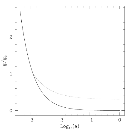
Figure 1: The absolute value of ${\bf g}/g_{{}_{0}}$ in the limit of small density fluctuations as a function of $a$ in an $\Omega=1$ matter dominated universe. The solid curve is the behavior according to Newtonian dynamics. The dotted curve is obtained when MOND is activated at $|{\bf g}|<g_{{}_{0}}$.

3.1 Epoch of MOND domination

The fluctuations in the Newtonian gravitational force field over a spherical region of physical radius $r=ax$ and density contrast $\delta$ are $g_{{}_{N}}\sim G\delta\bar{M}/(ax)^{2}$, where $\bar{M}\sim\bar{\rho}(ax)^{3}$. Since $\bar{\rho}\sim 1/a^{3}$, $g_{{}_{N}}$ decreases with time if $\delta\sim t^{\alpha}$ with $\alpha<2$. In linear Newtonian theory, $\alpha\leq 1$ and so at early enough times $g_{{}_{N}}>g_{{}_{0}}$ and the fluctuations would be in the Newtonian regime. At later times $g_{{}_{N}}$ drops below $g_{{}_{0}}$ and the fluctuations enter the MOND regime. Here we determine the redshift at which fluctuations on a comoving scale $x$ become MOND dominated. Assume that the transition epoch between Newtonian dynamics and MOND occurs early enough so that $\Omega\approx 1$, an assumption that will be justified below. The initial density field in the Newtonian regime is gaussian and characterized by the power-spectrum, $<|\delta_{k}|^{2}>$, where $\delta_{k}$ is the Fourier transform of the density as a function of the wavenumber, $k$. If the power-spectrum is a power-law of index $-3<n<1$, then the $rms$ value of the density field smoothed on a comoving scale $x$ at redshift $z$ is approximately

$$\sigma(x,z)=a(z)\left(\frac{x}{x_{{}_{0}}}\right)^{-\frac{n+3}{2}}\;,$$ (14)

where the redshift dependence through $a(z)=1/(1+z)$ follows from linear Newtonian theory if $\Omega=1$, and the scale $x_{{}_{0}}$ sets the amplitude of the fluctuations. According to either (3) or $g_{{}_{N}}\sim G\delta\bar{M}/{r^{2}}$, the $rms$ of $g_{{}_{N}}$ on a scale $x$ is

$$\sigma_{g}\sim\frac{3}{2}H^{2}ax\sigma\;.$$ (15)

The redshift, $z_{{}_{\rm mond}}$, at which $g_{{}_{N}}=g_{{}_{0}}=fR_{H}H_{{}_{0}}^{2}$ is then

$$z_{{}_{\rm mond}}=\frac{2}{3}f\frac{R_{H}}{x_{{}_{0}}}\left(\frac{x}{x_{{}_{0}}}\right)^{\frac{n+1}{2}}-1\;.$$ (16)

So if $n<-1$ then fluctuations on small scales enter the MOND regime before large scale fluctuations. For $n>-1$ the interpretation that large scales become MOND dominated earlier is somewhat vague. It is hard to visualize a large scale fluctuation in the MOND regime while the superimposed small scale fluctuations are still Newtonian. A more appropriate interpretation is that for $n>-1$ the volume of space containing fluctuations in the MOND regime is mainly made up of large regions separated by small scale fluctuations that are still Newtonian. This interpretation is sustained by the following argument. Since in the Newtonian regime ${\bf g}$ is gaussian, the probability that a spherical region of radius $x$ becomes MOND dominated at time $t$ is,

$$P\propto\int_{{}_{0}}^{g_{{}_{0}}/\sigma_{g}}\exp\left(-y^{2}/2\right)y^{2}\,{\rm d}y\;.$$ (17)

According to (15), $\sigma_{g}\propto x^{-(n+1)/2}$ so if $n>-1$ then $P$ increases with scale, meaning that the fraction of space already in MOND is made up of large regions. If $n<-1$ then $P$ decreases with scale and MOND penetrates small regions before it dominates the whole space.

Fluctuations enter the MOND regime at a relatively early time. Taking $x_{{}_{0}}\sim 10\rm{h^{-1}Mpc}$ and $R_{H}\sim 3000\rm{h^{-1}Mpc}$ then, according to (16), the transition into MOND occurs at $z>f200$, on scales $\lower 2.15277pt\hbox{$\;\buildrel>\over{\sim}\;$}10\rm{h^{-1}Mpc}$ if $n>-1$, and $\lower 2.15277pt\hbox{$\;\buildrel<\over{\sim}\;$}10\rm{h^{-1}Mpc}$ if $n<-1$. In a CDM-like power-spectrum the effective power-index on scales $\lower 2.15277pt\hbox{$\;\buildrel>\over{\sim}\;$}20\rm{h^{-1}Mpc}$ is $n\lower 2.15277pt\hbox{$\;\buildrel>\over{\sim}\;$}-1$ and changes to $-3<n\lower 2.15277pt\hbox{$\;\buildrel<\over{\sim}\;$}-1$ on smaller scales. For this type of power-spectrum the transition into MOND of all scales occurs at an early time when the density fluctuations are still small and $\Omega\approx 1$. This considerably simplifies our task of estimating the density power-spectrum in the MOND regime in the next subsection.

3.2 power-spectrum in the MOND regime at early times

MOND gives accelerations $\propto\sqrt{g_{{}_{0}}g_{{}_{N}}}>g_{{}_{N}}$, leading to faster growth rates than Newtonian gravity. So we expect a break in the shape of the power-spectrum at the scale just entering MOND. Assuming a power-law power-spectrum, $<|\delta_{k}|^{2}>\sim k^{n}$, in the Newtonian regime we estimate the power-index of the density fluctuations after they become MOND dominated. Consider the $rms$ value, $\tilde{\sigma}(x,a)$, of the density field over any scale $x$. Suppose that at redshift $z_{i}\gg 1$ fluctuations on all scales were Newtonian so that $\tilde{\sigma}=\sigma(x,z_{i})$, where $\sigma$ is given by (14). Let $x_{{}_{\rm mond}}(z)$ be the scale just entering the MOND regime at redshift $z<z_{i}$. For simplicity we consider the case $n<-1$, so at $x>x_{{}_{\rm mond}}$ the evolution is Newtonian and $\tilde{\sigma}=\sigma$. A fluctuation on a scale $x<x_{{}_{\rm mond}}$ entered MOND at redshift $z_{x}>z$. As we have seen in the previous subsection fluctuations on a wide range of scales become MOND dominated at an early enough time so that $\Omega\approx 1$. In an $\Omega\approx 1$ universe, the growth factors in the Newtonian and MOND regimes are $\delta\sim a$ and $\delta\sim a^{2}$, respectively. So, from $z_{i}$ until $z_{x}$ the fluctuation grew by a factor of $(a_{x}/a_{i})$, while from $z_{x}$ until $z$ it grew by $(a/a_{x})^{2}$, where $a_{i}=a(z_{i})$, $a_{x}=a(z_{x})$, and $a=a(z)$. So for $x<x_{{}_{\rm mond}}$,

$$\tilde{\sigma}(x,a)=\left(\frac{a}{a_{x}}\right)^{2}\left(\frac{a_{x}}{a_{i}}\right)\sigma(x,a_{i})\;.$$ (18)

According to (16)

$$\frac{a}{a_{x}}=\left(\frac{x_{{}_{\rm mond}}}{x}\right)^{-\frac{n+1}{2}}$$ (19)

and

$$\tilde{\sigma}(x,a)=a\left(\frac{x_{{}_{\rm mond}}}{x_{{}_{0}}}\right)^{-\frac{n+1}{2}}\left(\frac{x}{x_{{}_{0}}}\right)^{-1}\;,$$ (20)

so the power-index in the MOND regime is $n_{{}_{\rm mond}}=-1$. A similar argument for $n>-1$ yields the same result. Therefore the power-index in the MOND regime is independent of the value of $n$. A general power-spectrum can be approximated as a power-law over any limited range of scales where our result applies. Therefore, MOND drives the power-spectrum towards $k^{-1}$ independent of its shape in the Newtonian regime.

The treatment here ignored mode-coupling and assumed that all fluctuations became MOND dominated when $\Omega$ was still very close to unity. Although the simulations presented in the next section do not show strong mode-coupling for low values of $g_{{}_{0}}$, the shape of the power-spectrum derived here should serve as a general indication only.

4 Results from N-body simulations

In this section we study the general evolution of fluctuations under MOND by means of N-body simulations. This is done by adapting a particle-mesh (PM) N-body code originally written by E. Bertschinger to solve the Newtonian equations (Bertschinger & Gelb 1991). At each time step, the code readily provides the irrotational component of ${{\bf g}}_{{}_{N}}$ from the density field as estimated on a grid from the particle distribution. We adapt the code by adding a routine to compute the gravitational field ${\bf g}$ from ${{\bf g}}_{{}_{N}}$ using the relation (7). We also incorporate the time dependent functions in the MOND equations in a leapfrog time integration scheme to move the particles to the next time step.

Table 1: Details of the six simulations. Each simulation contained $64^{3}$ particles in a cubic box of $128{\mathrm{h}}^{-1}{\mathrm{M}pc}$ on the side. The $rms$ value, $\sigma_{8}$, of density fluctuations in spheres of radius $8\rm{h^{-1}Mpc}$ is measured from the output of each simulation at the final time.

simulation	gravity	$g_{{}_{0}}/(1.2\times 10^{-8}{\mathrm{c}m/s}^{2})$	$\Omega_{0}$	$\sigma_{8}$
I	MOND	1	1	3.9
II	MOND	1	0.03	4.83
III	MOND	1	1	1.16
		($10^{-6}\delta_{\mathrm{i}nitial}$)
IV	MOND	1/12	1	1.08
V	MOND	1/12	0.03	1.01
VI	Newton	0	1	0.86

Five MOND simulations with different values of $g_{{}_{0}}$ and $\Omega_{0}\equiv\Omega(a=1)$ were run. For comparison, a simulation with Newtonian gravity was also run. The simulations started with gaussian initial conditions generated from the CDM power-spectrum with $H_{{}_{0}}=50\rm{h^{-1}Mpc}$ and $\Omega_{0}=1$. Each simulation contained $64^{3}$ particles in a cubic box of $128\rm{h^{-1}Mpc}$ on the side. The CDM power spectrum on the large scales probed by the box is close to $k^{-1}$ as motivated by our result for the density power-spectrum in the MOND regime at early times. The parameters of each simulation are written in Table 1. Except simulation III, all simulations started with the same initial conditions which were normalized so that the density field in Newtonian simulation at the final time had an $rms$ value of $\sigma_{8}=0.86$ in spheres of radius $8\rm{h^{-1}Mpc}$. In simulation III, the amplitude of the initial conditions was reduced by a factor of $10^{6}$. Simulations with $\Omega_{0}=1$ and $0.03$ started at $a=0.049$ and $0.01$, respectively. At these two time the linear Newtonian density growth factor, $D$, was the same for the two values of $\Omega_{0}$. For the high $g_{{}_{0}}$, this choice of the starting time of the simulations corresponds roughly to the epoch at which fluctuations on all scales become MOND dominated according to our estimate in section 3.2. The particle distribution at this time was obtained using the Zel’dovich approximation. We are interested in comparing the net dynamical effect of decreasing $g_{{}_{0}}$ and so we start MOND simulations with low and high $g_{{}_{0}}$ at the same value of $D$.

Figure 2: The particle distribution in a slice of thickness $2.56\rm{h^{-1}Mpc}$ through the simulations at the final time. The panels in a clockwise order correspond to simulations I—VI listed in the table 1. See fig2.gif

Fig. 2 show the particle distribution in a slice in the simulations at $a=1$. This figure demonstrates that MOND with the standard value of $g_{{}_{0}}\approx 1.2\times 10^{-8}{\mathrm{c}ms^{-2}}$ (bottom and middle panels to the left) yields high clustering at the present time, for both $\Omega_{0}=1$ and $0.03$. Lowering the amplitude of the initial fluctuations by a factor of $10^{6}$ reduces the clustering at the present time but severely washes out small scale fluctuations (top panel to the left). For both values of $\Omega_{0}$, MOND with a smaller value for $g_{{}_{0}}$ produces particle distribution (top and middle panels to the right) similar to Newtonian dynamics (bottom panel to the right). The values of $\sigma_{8}$ measured from simulations at the final time are listed in Table 1. Fig. 3 shows $\Delta^{2}(k)=Vk^{3}<|\delta_{k}|^{2}>/2\pi^{2}$ where $V$ is the volume of the simulation box (Peacock 1999). This quantity gives the contribution to the variance per $\ln(k)$. The MOND curves with low $g_{{}_{0}}$ (IV and V) follow the shape of the Newtonian curve (VI).

Figure 3: The variance $\Delta^{2}(k)=k^{3}<|\delta_{k}|^{2}>/(2\pi^{2})$ of density fields per $\ln(k)$ from the simulations at the final time. The solid, long-dashed, short-dashed, dotted, dot-short-dashed, and dot-long-dashed and lines correspond respectively to simulations I–VI.

Figure 4: The peculiar velocity vs. the “Newtonian” gravity field ${\bf g}_{{}_{N}}$ obtained from the density contrast using (6). The panels show fields from simulations II ($\Omega_{0}=0.03$, high $g_{{}_{0}}$), IV ($\Omega_{0}=1$, low $g_{{}_{0}}$), V ($\Omega_{0}=0.03$, low $g_{{}_{0}}$), and VI (Newtonian), as indicated in the figure. The fields were smoothed with a Gaussian window of radius $8\rm{h^{-1}Mpc}$. The diagonal line in each panel is plotted to guide the eye. See fig4.gif

A common method for estimating the cosmological density parameter, $\Omega$, is the comparison between the measured peculiar velocity field and the “Newtonian” gravity field, ${\bf g}_{{}_{N}}$, inferred observed distribution of galaxies using (6) (see Strauss & Willick 1995 and references therein). Putting aside the issue of redshift distortions, linear Newtonian theory gives $f(\Omega){\bf u}=H{\bf g}_{{}_{N}}$, where $f(\Omega)\approx\Omega^{0.6}$ (e.g., Peebles 1980). This comparison has been done using several data sets with the conclusion that the observed velocity and gravity fields are tightly correlated. To test whether MOND can account for the correlation seen in the observations, we have performed a comparison between the velocity and “Newtonian” gravity field, ${\bf g}_{{}_{N}}$, computed from the simulations at the final time. The results are shown in Fig. 4. To avoid strong non-linearities, the fields were smoothed with a gaussian window of radius $8\rm{h^{-1}Mpc}$. The $rms$ values of the one dimensional ${\bf u}$ and $H{\bf g}_{{}_{N}}$ shown in the figure are $(\sigma_{u},\sigma_{g})=(1176,336)$, (450,302), (223,336), and (209,226) in ${\rm km\;s^{-1}}$, respectively, for the simulations II, IV, V, and VI. Simulation II is highly non-linear even on scales larger than $8\rm{h^{-1}Mpc}$ and the relative scatter between the fields is large. In the simulations with small $g_{{}_{0}}$, the correlation between the fields is tight for both $\Omega_{0}=1$ (simulation IV) and $\Omega_{0}=0.03$ (V). The scatter between the fields is larger than in the Newtonian simulation (VI), but it is negligible compared to observational uncertainties. The slope of the regression of $u_{x}$ on $Hg_{{}_{N,x}}$ is higher in simulation $IV$ than in the Newtonian simulation, $VI$. These two simulations have $\Omega_{0}=1$ but as is the case with rotational speeds of galaxies, MOND also accounts for larger velocities on large scales. These results indicate that MOND can be consistent with this type of analysis. In MOND, the slope of the regression of ${\bf u}$ on $H{\bf g}_{{}_{N}}$ is also a decreasing function of $\Omega$, but is not proportional to $f(\Omega)$. For example for the MOND simulation V with low $g_{{}_{0}}$ and $\Omega_{0}=0.03$, the slope is 0.55, instead of $0.25$ in linear Newtonian theory. Note that the relation (7) between ${\bf g}$ and ${\bf g}_{{}_{N}}$ implies that $|{\bf g}|\ll g{{}_{0}}$ in all MOND simulations, sustaining our conjecture that large scale fluctuations never leave the MOND regime. We have also computed the probability distribution function (PDF) of density field smoothed on $8\rm{h^{-1}Mpc}$. The shape of the PDF in the simulations with small $g_{{}_{0}}$ is very close to that in the Newtonian simulation.

The simulations shown so far were run assuming all particles enter the MOND regime at the same time. This captures the net dynamical effects of varying $g_{{}_{0}}$. However, a realistic MOND simulation should start at an early enough time when most particles are still Newtonian. A particle moves accroding to Newtonian dynamics, until the its peculiar gravitational (in absolute value), $g$, drops below $g_{{}_{0}}$. The subsequent motion of the particle is governed by MOND as long as $g<g_{0}$. We have run a suite of simulations with this recipe for modeling the transition into MOND. Of course the transition into MOND could be made a little smoother but in the lack of an exact model for how the transition occurs we choose to proceed assuming sudden transition. The simulations we have run correspond to the CDM power-spectrum used in the simulations shown in Fig. 2, and two scale-free power-spectra with power-indices, $n=-1$ and $n=1$. All simulations were run for $\Omega=0.03$ with the standard and low value of $g_{0}$. The initial conditions were normalized similarly to the Newtonian simulation in table 1. Slices of the particle distribution in these simulations are shown in Figs. 5 and 6, for $a=1$ and $a=0.1$, respectively. The particle distribution of the CDM simulation in Fig. 5 (bottom panels) is a little more evolved than in Fig. 2. Despite this, the particle distributions in the two simulations are very similar. This indicates that MOND becomes dominated at a similar epoch for all particles and that our estimate of this epoch used in the simulations shown in Fig. 2 is reliable.

Figure 5: The particle distribution in a slice of thickness $2.56\rm{h^{-1}Mpc}$ through the simulations at the final time, $a=1$. These simulations have $\Omega_{0}=0.03$ and started early enough when most particle were Newtonian. A particle became MOND dominated once its peculiar acceleration dropped below $g_{0}$. The panels on the left are for simulations run with standard $g_{0}$ while the panels on the right are with low $g_{0}$ (1/12 standard). Bottom, middle, and top rows correspond to power-spectra of CDM, $n=-1$, and $n=+1$, respectively. See fig5.gif

Figure 6: The same as the previous figure (5), but for simulations at $a=0.1$. See fig6.gif

5 Summary and discussion

Several arguments against MOND have been presented in the literature ( e.g., Felten 1984, van den Bosch et al. 2000, Mortlock & Turner 2001, Aguirre et al. 2001, Scott et al. 2001). The reader may decide for her/himself which of these arguments are compelling. Here we focus on examining the general properties of large scale structure under MOND and put aside the arguments presented in the literature against MOND. The value of $g_{{}_{0}}$ necessary to fit the rotation curves of galaxies produces far too much clustering and can be consistent with observations only with strong anti-bias. Decreasing $g_{{}_{0}}$ has two effects: 1) it pushes the epoch of MOND domination to later time, and 2) it reduces the typical accelerations produced by MOND forces. The simulations presented in this paper show that MOND with smaller $g_{{}_{0}}$ leads to large scale structure similar to Newtonian dynamics. This is encouraging for MOND since the standard paradigm based on Newtonian gravity and dark matter is successful at explaining many observations of the large scale structure and the galaxy population (e.g., Kauffman, Nusser & Steinmetz 1997, Benson et al. 2000, Diaferio et al. 2001) . Still one has to adopt a generalization of MOND, allowing for, or at least mimicking, a scale dependent $g_{{}_{0}}$. Sanders’ (2001) two-field theory for example can serve as a general framework for that purpose. In this theory the rapid growth of fluctuations in MOND is tamed by the coupling between the two fields. The amplitude of the initial conditions used in the simulations roughly matches the normalization implied by measurements of the cosmic microwave background anisotropies (Hu W., Sugiyama & Silk 1997). We have seen that by reducing the amplitude of the initial conditions by a large factor MOND with the standard value of $g_{{}_{0}}$ produces the correct $\sigma_{8}$, but causes a severe washing out of structure on scale of 10s of $\rm{h^{-1}Mpc}$. Therefore it seems necessary to decrease $g_{{}_{0}}$ to match the large scale structure.

Our goal here was to present general criteria for the consistency of MOND with large scale structure. Further study of MOND within a realsitic recipe for galaxy formation to clarify the role of (anti-) biasing remains to be done.

6 Acknowledgments

I thank Ed Bertschinger for allowing the use of his PM code, Simon White and Stacey McGaugh for useful comment. This research was supported by the Technion V.P.R Fund- Henri Gutwirth Promotion of Research Fund, and the German Israeli Foundation for Scientific Research and Development.

References

- [1] Aguirre A., Schaye J., Quataert E., 2001, accepted, ApJ, astro-ph/0105184
- [2] Begeman K.G., Broeils A.H., Sanders R.H. 1991, MNRAS, 249, 523
- [3] Bekenstein J., Milgrom M., 1984, ApJ, 286, 7
- [4] Benson A.J., Cole S., Frenk C.S., Baugh C.M., Lacey C.G., 2000, MNRAS, 311, 793
- [5] Bertschinger E., Gelb J.M, 1991, Computers in Physics, 5, 164
- [6] Binney J.J., Tremaine S., 1987, Galactic Dynamics, Princeton University Press
- [7] de Blok W.J.G., McGaugh S.S., 1998, ApJ, 508, 132
- [8] de Blok W.J.G., McGaugh S.S., Bosma A., Rubin V.C., 2001, ApJL, 552, 23
- [9] Diaferio A., Kauffman G., Balogh M.L., White S.D.M., Schade D., Ellingson E., 2001, MNRAS, 323, 999
- [10] Felten J.E., 1984, ApJ, 286, 3
- [11] Flores R.A. Primack J.P., 1994, ApJ, 427,1
- [12] Hu W., Sugiyama N., Silk J., 1997, Nature, 386, 37
- [13] Kauffmann G., Nusser A., Steinmetz M., 1997, MNRAS, 286, 795
- [14] Milgrom M., 1983, 270, 365
- [15] Milgrom M., Braun E., 1988, ApJ, 334, 130
- [16] McGaugh S.S, 1999, ApJ, 523, L99
- [17] Moore B.,1994, Nature, 370, 629
- [18] Mortlock D.J., Turner E.L., 2001, MNRAS, 327, 557
- [19] Peacock J.A, 1999, Cosmological Physics, Cambridge University Press
- [20] Peebles J.P.E, 1980 Large Scale Structure, Princeton University Press
- [21] Sanders R.H., 1996, ApJ, 473, 117
- [22] Sanders R.H., 1998, MNRAS, 296, 1009
- [23] Sanders R.H., Verheijen M.A.W., 1998, ApJ, 503, 97
- [24] Sanders R.H., 2001, astro-ph/0011439
- [25] Scott D., White M., Cohn J., Pierpaoli E., 2001, astro-ph/014435
- [26] Strauss M.A., Willick J.A, 1995, Physics Reports, 261,271
- [27] van den Bosch F.C., Dalcanton J.J., 2000, ApJ, 534, 146