Scaling and correlation analysis of galactic images

Abstract

Different scaling and autocorrelation characteristics and their application to astronomical images are discussed: the structure function, the autocorrelation function, Fourier spectra and wavelet spectra. The choice of the mathematical tool is of great importance for the scaling analysis of images. The structure function, for example, cannot resolve scales which are close to the dominating large-scale structures and can lead to the wrong interpretation that a continuous range of scales with a power law exists. The traditional Fourier technique, applied to real data, gives very spiky spectra, in which the separation of real maxima and high harmonics can be difficult. We recommend as the optimal tool the wavelet spectrum with a suitable choice of the analysing wavelet. We introduce the wavelet cross-correlation function which enables to study the correlation between images as a function of scale. The cross-correlation coefficient strongly depends on the scale. The classical cross-correlation coefficient can be misleading if a bright, extended central region or an extended disk exists in the galactic images.

An analysis of the scaling and cross-correlation characteristics of 9 optical and radio maps of the nearby spiral galaxy NGC 6946 is presented. The wavelet spectra allow to separate structures on different scales like spiral arms and diffuse extended emission. Only the images of thermal radio emission and H$\alpha$ emission give indications of 3-dimensional Kolmogorov-type turbulence on the smallest resolved scales (160–800 pc). The cross-correlations between the images of NGC 6946 show strong similarities between the images of total radio emission, red light and mid-infrared dust emission on all scales. The best correlation is found between total radio emission and dust emission. Thermal radio continuum and H$\alpha$ emission are best correlated on a scale of about $1\arcmin\simeq 1.6$ kpc, the typical width of a spiral arm. On a similar scale, the images of polarised radio and H$\alpha$ emission are anticorrelated, which remains undetected with classical cross-correlation analysis.

1 Introduction

The increasing resolution of optical, radio, infrared and X-ray telescopes over the past decades has greatly improved the details visible in astronomical objects in many wavelength ranges. The large variety in the structure of external galaxies, which have bars, bright central regions, spiral arms with clumpy star-forming regions, long known from optical photographs, can now also be identified in radio, X-ray and IR continuum, and in spectral lines of ionised (${\rm H\,\scriptstyle II}$), atomic (${\rm H\,\scriptstyle I}$) and molecular (CO) gas components. How these different constituents in a galaxy are related is a question to which continuous study has been devoted.

The detection of similar structures in widely separated energy ranges gives important information on physical processes and their interplay. For example, the degree of correlation between the H$\alpha$ emission and the free-free emission in radio continuum tells us about the amount of absorption in the optical range. The similarity of far-infrared and radio continuum emission components (e.g. in the nearby spiral galaxy M 31) indicates that magnetic fields are not anchored in the warm medium, but in cool gas clouds (Hoernes, Berkhuijsen & Xu 1998). Also emission in the CO line is correlated with radio continuum emission in spiral arms of M 31, but it is anticorrelated with the polarised radio emission (Berkhuijsen, Bajaja & Beck 1993).

Anticorrelations are possibly even more interesting than correlations. In the spiral galaxy NGC 6946 a striking anticorrelation between the optical spiral arms and the “magnetic arms” seen in radio polarisation was discovered by Beck & Hoernes (1996). Although obvious to the eye, the analysis of this phenomenon needs sophisticated techniques. Based on wavelet analysis, Frick et al. (2000) showed that the “magnetic arms” are phase-shifted images of the optical arms. Dynamo action is able to generate such structures (Rohde, Beck & Elstner 1999).

The existence of a correlation, anticorrelation or non-correlation has important consequences for the interpretation of observable quantities which emerge from a combination of physical quantities. For example, Faraday rotation ($RM$) of polarised radio waves is due to the product of electron density ($n_{\rm e}$) and the magnetic field component along the line of sight ($B_{\parallel}$), averaged along the line of sight. Knowledge of $<n_{\rm e}>$ (e.g. from dispersion measures of pulsars) is not sufficient to determine the strength of $<B_{\parallel}>$ unless it is known whether $n_{\rm e}$ and $B_{\parallel}$ are correlated, anticorrelated or non-correlated. If the anticorrelation observed on the scale of spiral arms holds also on small scales, the field strengths derived from Faraday rotation data of pulsars are too small (Beck 2001).

Relations between images are generally analysed with the pixel-to-pixel correlation function. However, this method gives little information in the case of an anticorrelation on the scale of spiral arms, like in NGC 6946, or when the diffuse emission on larger scales (e.g. in total radio emission) has no counterpart in the other image (e.g. polarised radio emission).

Another interesting subject is turbulence in the interstellar medium of galaxies, which has been studied by analysing structure functions of appropriate images. Observations of radio-wave scintillations in the Milky Way have revealed the existence of density irregularities in the diffuse ionised gas with scale sizes of $\geq 10^{18}$ cm (0.3 pc) down to $10^{7}$ cm. The spectrum of the irregularities is consistent with the spectrum of three-dimensional Kolmogorov turbulence (Spangler 1999). A spectrum with the same slope was found by Minter & Spangler (1996) for both the turbulent fluctuations in electron density and in Faraday rotation measure observed in the same area in the Milky Way. The outer scale of these fluctuations is 4 pc. For larger scales up to about 80 pc Minter & Spangler found a flatter spectrum. As turbulent scales larger than about 100 pc are difficult to observe in our Galaxy, it is still unknown whether the Kolmogorov spectrum extends to large scales. The analysis of images of external galaxies may give us this information.

In laboratory experiments extremely long data series are used to get reliable statistics for the slopes of structure functions of high order in the inertial range (Monin & Yaglom 1971, 1975; Frisch 1995). The analysis of turbulence in astronomical objects requires observational data of very high quality and high angular resolution. The excellent data set on the external galaxy NGC 6946 seems well suited for a study of turbulence on large scales. In a first attempt Beck, Berkhuijsen & Uyanıker (1999) analysed the high-resolution radio continuum maps of this galaxy using the structure function. They found spectra consistent with two-dimensional turbulence in the radio continuum emission on scales between $0\aas@@fstack{\prime}5$ (twice the beam size) and $5\aas@@fstack{\prime}0$. In this paper, however, we show that in the case of images with pronounced structures on scales less than 20$\times$ the size of the telescope beam, like the bright central area and spiral arms covering most of the available images, the structure function is not the best analysing tool because it does not well resolve these scales. The lack of spectral resolution and the relatively poor statistics (i.e. a small ratio of image size to beam size) influence the slope of the derived structure function, making the interpretation difficult. As astronomical observations are limited in resolution and extent, the mathematical tools used for their analysis have to be chosen carefully and the results need a critical evaluation.

During the last decade a new mathematical tool has been developed, wavelet analysis which enables the detection of structures of different scales in data sets. First applications to astronomical objects showed that wavelets are effective in time series analysis (Foster 1996; Frick et al. 1997a,b), denoising (Tenorio et al. 1999; Chen et al. 2000) and structure detection (Frick et al. 2000).

We have applied two-dimensional wavelet analysis to images of NGC 6946 at various wavelengths. Our goal is not only to detect the dominant scales in this galaxy, but also to see if wavelets can be useful to determine the statistical characteristics for given scales in the maps. The observation of magnetic arms situated in between the gaseous arms, leading to an absence of classical cross-correlation between the corresponding images in spite of their similarity, stimulated this research.

The paper is organized as follows. In Sect. 2 we present the wavelets as a tool of scaling analysis. Their relationship with spectra and structure functions is explained in Sect. 3, and how wavelets can be used for correlations at a given scale is shown in Sect. 4. In the second part of the paper the wavelet analysis is applied to images of the nearby galaxy NGC 6946 (Sect. 5.1). First its spectral characteristics are discussed in Sect. 5.2, then the correlations between pairs of images are presented in Sect. 5.3. The results are discussed in Sect. 6.

2 Wavelets as a tool for scaling analysis

Wavelet analysis is based on a space-scale decomposition using the convolution of the data with a family of self-similar basic functions that depend on two parameters, scale and location. It can be considered as a generalization of the Fourier transformation, which uses harmonic functions as a one-parametric functional basis, characterized by frequency, or in the case of a space function, by the wavevector $\vec{k}$. The wavelet transformation also uses oscillatory functions, but in contrast to the Fourier transform these functions rapidly decay towards infinity. The family of functions is generated by dilations and translations of the mother function, called the analysing wavelet. This procedure provides self-similarity, which distinguishes the wavelet technique from the windowed Fourier transformation, where the frequency, the width of the window and its position are independent parameters.

We consider the continuous wavelet transform, which in the two-dimensional case can be written in the form

$$W(a,\vec{x})={1\over{a^{\kappa}}}\int_{-\infty}^{+\infty}\int_{-\infty}^{+\infty}f(\vec{x}^{\prime})\psi^{*}\left({{\vec{x}^{\prime}-\vec{x}}\over a}\right)d\vec{x}^{\prime}.$$ (1)

Here $\vec{x}=(x,y)$, $f(\vec{x})$ is a two-dimensional function, for which the Fourier transform exists (i.e. square integrated), $\psi(\vec{x})$ is the analysing wavelet (real or complex, ^∗ indicates the complex conjugation), $a$ is the scale parameter, and $\kappa$ is a normalization parameter which will be discussed below.

For later considerations the relation between the wavelet and the Fourier decomposition will be useful. The 2-D Fourier transform $\hat{f}(\vec{k})$ of the function $f(\vec{x})$ is defined as

$$\hat{f}(\vec{k})=\int_{-\infty}^{+\infty}\int_{-\infty}^{+\infty}f(\vec{x})e^{-i\vec{k}\vec{x}}d\vec{x},$$ (2)

where $\vec{k}=(k_{x},k_{y})$ is the wavevector. Then the inverse Fourier transform is

$$f(\vec{x})={1\over{4\pi^{2}}}\int_{-\infty}^{+\infty}\int_{-\infty}^{+\infty}\hat{f}(\vec{k})e^{i\vec{k}\vec{x}}d\vec{k}$$ (3)

and the wavelet coefficients (1) can be expressed as

$$W(a,\vec{x})={a^{2-\kappa}\over{4\pi^{2}}}\int_{-\infty}^{+\infty}\int_{-\infty}^{+\infty}\hat{f}(\vec{k})\hat{\psi}^{*}(a\vec{k})e^{i\vec{k}\vec{x}}d\vec{k}.$$ (4)

We restrict our analysis to the use of isotropic wavelets. It means that the analysing wavelet is an axisymmetric function $\psi=\psi(\rho),\ \rho=\sqrt{x^{2}+y^{2}}$. The choice of the wavelet function depends on the data and on the goals of the analysis. For spectral analysis wavelets with good spectral resolution (i.e. well localized in Fourier space, or having many oscillations) are preferable, for local structure recognition a function, well localized in the physical space, is preferable. (Note that the spectral resolution $\Delta k$ and the space resolution $\Delta x$ are strongly related and are restricted by the uncertainty relation $\Delta x\Delta k\geq 2\pi$.) An obligatory property of the wavelet is the zero mean value $\int\int\psi(x,y)dxdy=0$.

In the case under consideration the choice of the wavelet was determined by the wish to have more independent points for further structure analysis which led to a simple real isotropic wavelet with a minimal number of oscillations, known as the Mexican Hat

$$\psi(\rho)=(2-\rho^{2})e^{-\rho^{2}/2}.$$ (5)

We shall refer to this function as MH.

For a better separation of scales (to analyse spectra and to find the scale of dominant structures) another isotropic wavelet was used which is defined in Fourier space by the formula

$$\hat{\psi}(\vec{k})=\left\{\begin{array}[]{l@{\qquad: \qquad}l}\cos^{2}({\pi\over 2}\log_{2}{k\over{2\pi}})&\pi<|\vec{k}|<4\pi\\ 0&|\vec{k}|<\pi,|\vec{k}|>4\pi\ .\end{array}\right.$$ (6)

The function is localized in Fourier space in a ring with a median radius $2\pi$ and vanishes for $|\vec{k}|<\pi$ and $|\vec{k}|>4\pi$. This wavelet definition provides a relatively good spectral resolution, it will be referred to as PH (it is our Pet Hat). In physical space the PH wavelet is obtained by numerical integration of (6). Both wavelets MH and PH are shown in Fig. 1.

Figure 1: Two isotropic wavelet functions used in this paper: the MH wavelet (thin line) and the PH wavelet (thick line).

The wavelet transform (1) is unique and reversible which means that the analysed function $f(x,y)$ can be reconstructed from its wavelet decomposition. In our analysis we do not need the inverse transform and do not give the reconstruction formula. (An extended description of continuum wavelet transform can be found in e.g. Holschneider (1995) and Torresani (1995).)

To illustrate how wavelets decompose the image in different scales we show in Fig. 2 the optical broadband emission image of the galaxy NGC 6946 and its wavelet coefficients $W(a,\vec{x})$ for three different scales $a$. For this example the PH wavelet was used.

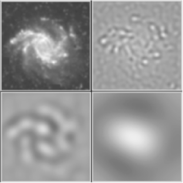
Figure 2: NGC 6946. Map of the optical emission in red light (central region subtracted) and its wavelet decompositions for 3 different scales: 0$\aas@@fstack{\prime}$5, 1$\aas@@fstack{\prime}$4 and 4′. The size of each image is $11\arcmin\times 11\arcmin$.

3 Spectra and structure functions

In the studies of scaling properties of turbulence a commonly used characteristic of a turbulent field is the spectral energy density $E(k)$ which includes the energy $F(\vec{k})=|\hat{f}(\vec{k})|^{2}$ of all Fourier harmonics with wavenumbers $\vec{k}$, for which $|\vec{k}|=k$

$$E(k)=\int_{|\vec{k}|=k}F(\vec{k})d\vec{k}\ .$$ (7)

The spectral energy is related to the autocorrelation function

$$C(\vec{l})=\int_{-\infty}^{+\infty}\int_{-\infty}^{+\infty}f(\vec{x})f(\vec{l}-\vec{x})d\vec{x}$$ (8)

by its Fourier transform

$$F(\vec{k})=\hat{C}(\vec{k})=\int_{-\infty}^{+\infty}\int_{-\infty}^{+\infty}C(\vec{l})e^{-i\vec{k}\vec{l}}d\vec{l}\ .$$ (9)

The vector $\vec{l}$ defines the shift of the image in the convolution (8) and is the scale parameter. In the important case of isotropic turbulence the autocorrelation function depends only on the distance between two points $C(\vec{l})=C(l)$, and the spectral energy depends only on the modulus of the wavevector $F(\vec{k})=F(k)$. Then these two functions are related by the Hankel transform

$$F(k)=2\pi\int_{0}^{\infty}C(l)J_{0}(kl)ldl\ ,$$ (10)

where $J_{0}$ is the Bessel function and $E(k)=2\pi kF(k)$.

Another often used characteristic for scaling studies is the structure function defined for arbitrary order $q$ as

$$S_{q}(l)=\ <(f(\vec{x})-f(\vec{x}-\vec{l}))^{q}>_{|\vec{l}|=l}\ ,$$ (11)

where the brackets $<...>$ mean the average value. Calculation of high-order structure functions requires a high accuracy of the initial data. In the case of maps of external galaxies, where a relatively small number of grid points is available and the noise is significant, only the second-order function $S_{2}$, corresponding to the energy spectrum (7), can be discussed.

In the wavelet representation the scale distribution of the energy can be characterized by the wavelet spectrum, defined as the energy of the wavelet coefficients of scale $a$ of the whole physical plane

$$M(a)=\int_{-\infty}^{+\infty}\int_{-\infty}^{+\infty}|W(a,\vec{x})|^{2}d\vec{x}\ .$$ (12)

The wavelet spectrum can be related to the Fourier spectrum. Using (4) one can easily rewrite (12) in the form

$$M(a)={a^{4-2\kappa}\over{16\pi^{4}}}\int_{-\infty}^{+\infty}\int_{-\infty}^{+\infty}|\hat{f}(\vec{k})|^{2}|\hat{\psi}(a\vec{k})|^{2}d\vec{k}\ .$$ (13)

This relation shows that the wavelet spectrum is a smoothed version of the Fourier spectrum. In the isotropic case (13) has a more simple form

$$M(a)={a^{4-2\kappa}\over{8\pi^{3}}}\int_{0}^{\infty}E(k)|\hat{\psi}(ak)|^{2}dk\ .$$ (14)

A generic property of fully developed small-scale turbulence is the presence of an inertial range of scales in which the energetic characteristics $E(k)$, $S_{2}(l)$ and $M(a)$ follow power laws. Let us consider the relation between the spectral indices of these characteristics. Let the structure function follow a power law

$$S_{2}(l)\sim l^{\lambda}\ .$$ (15)

Then, $F(k)\sim k^{-\lambda-2}$ and the spectral energy density exhibits a power law

$$E(k)\sim k^{-(\lambda+1)}\ .$$ (16)

The behaviour of the wavelet spectrum M(a) depends on the normalization $\kappa$ in definition (1). We will use $\kappa=2$, which gives the same power law for the wavelet spectrum as for the structure function

$$M(a)\sim a^{\lambda}\ .$$ (17)

Choosing $\kappa=3/2$ the wavelet spectrum becomes $M(a)\sim a^{\lambda+1}$, which is convenient if the result should be compared with the Fourier spectrum $E(k)$. It should be noted that the scale parameter $a$ commonly used in wavelets has the same meaning as the distance $l$ in the autocorrelation (8) or structure function (11). Below we shall normally use the character $a$ for the scale parameter in any spectral characteristic.

An important remark concerns the power-law search in spectra. Every wavelet has its own spectral portrait and the tail of the corresponding spectral energy distribution often itself follows a power law. The power index of this law defines the absolute limit of the spectral slope that can be obtained using the given wavelet.

Note that the traditional calculation of the structure function $S_{2}$ following (11) can be interpreted as the calculation of the wavelet spectrum (12), obtained using a “special” anisotropic wavelet, which gives the difference between two delta functions separated by the unit distance

$$\psi(\vec{x},\vec{e})=\delta(\vec{x})-\delta(\vec{x}-\vec{e})\ ,$$ (18)

where $\vec{e}$ is the unit vector. This quasi-wavelet (18) is a bad wavelet in the sense that being very well localized in physical space it has inevitably a very bad spectral resolution. This means that structure functions give a poor scale separation and as a result they are always very smooth. This is why the structure functions can be useful only in the case of a well developed range of scales for which a power law is established.

We conclude this section with an illustrative example which is relevant to further data analysis. In Fig. 3a two images are presented, the second one being a phase-shifted copy of the first one. The spectral properties of these two images are identical and are shown in Fig. 3b. The upper curve shows the structure function $S_{2}$ (11), which is almost flat over a large range of scales. A steep decrease appears at large scales when the distance $l$ surpasses the total size of the structure. The next two curves reproduce the wavelet spectra obtained with different wavelets, MH (5) and PH (6). The graphs clearly illustrate the increase of spectral resolution: some maxima are indicated in the MH spectrum and three maxima are well pronounced in the PH spectrum. These maxima correspond to the scale of the width of an individual spoke in the image, the scale of its length and the global scale of the structure. The last (lower) curve shows the Fourier spectrum, calculated via the Hankel transform (10) of the autocorrelation function (8). It displays of course the best spectral resolution but includes the upper harmonics – two maxima at $a<0.25$ are the double harmonics of the central structure. Note that the Fourier spectrum is shown versus the physical scale $a$ which can be interpreted as the wavelength, $a=2\pi/k$, thus the high frequencies are to the left (small $a$).

This example illustrates the usual problem of Fourier presentation of observational data – real data give very spiky spectra and the interpretation of different maxima in them is difficult. A reliable choice of wavelets leads to smooth spectra which nevertheless clearly indicate the dominant scales in the analysed data. Note also that the global scale indicated by the structure function and the wavelets at $a\approx 3$ is not visible in the Fourier spectrum – the size of the image is too small to contain the corresponding Fourier harmonic.

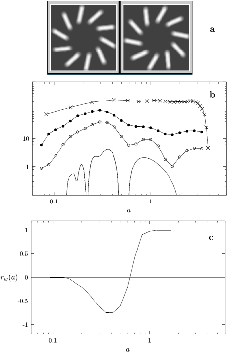
Figure 3: Spectral and correlation characteristics of artificial images. a Test images with sides of length 2; b spectral characteristics of a single image: second-order structure function (crosses), MH wavelet spectrum (black dots), PH wavelet spectrum (circles), Fourier spectrum (line) (the spectra are shifted along the vertical axis for better presentation), $a=2\pi/k$; c wavelet cross-correlation coefficient.

4 Wavelet cross-correlations

In this section we discuss correlations of images of the same extragalactic object at different wavelengths and how they can be quantified.

Let us consider two images (maps), $f_{1}(x,y)$ and $f_{2}(x,y)$, with the same angular resolution and the same number of pixels. The simplest way for a linear correlation study is the direct calculation of the correlation coefficient point by point (pixel by pixel)

$$r_{p}={{\sum(f_{1i}-<f_{1}>)(f_{2i}-<f_{2}>)}\over{((f_{1i}-<f_{1}>)^{2}(f_{2i}-<f_{2}>)^{2})^{1/2}}}\ .$$ (19)

The accuracy of this estimate depends on the degree of correlation and on the number of independent points $n$ (see for example Edwards (1979))

$$\Delta r={{\sqrt{1-r^{2}}}\over{\sqrt{n-2}}}\ .$$ (20)

Here $n$ is the ratio of the map area to the area of the beam ($n\simeq 1700$ in the maps discussed in Section 5).

The “pixel by pixel” correlation coefficient is a global characteristic which contains all the scales present in the images, including the largest one which reflects the fact that the centre of the extended intensity distribution is nearly at the same position at most wavelengths (see the last panel of Fig. 2).

It is interesting to investigate whether the correlation coefficient depends on scale. Therefore we introduce the correlation coefficient for a given scale $a$

$$r_{w}(a)={{\int\int W_{1}(a,\vec{x})W_{2}^{*}(a,\vec{x})d\vec{x}}\over{(M_{1}(a)M_{2}(a))^{1/2}}}\ .$$ (21)

To estimate the error $\Delta r_{w}(a)$ we use formula (20) taking $n=(L/a)^{2}$, where $L$ is the size of the map.

To illustrate the behaviour of this wavelet correlation (i.e. correlation on a given scale) let us return to the example given in Fig. 3. The two images shown in the upper panel have an angular shift $\pi/10$ (the spokes in the second map are just in between those in the first one). Calculating the “pixel by pixel” correlation coefficient yields $r_{p}=-0.01$. This vanishing value of the correlation coefficient reflects the fact that the bright details of both images occupy a small part of the image and do not overlap. At the same time it is clear that the images are very well correlated in general, because the images present two identical structures, one of which is rotated. In Fig. 3c we present the wavelet correlation coefficient $r_{w}(a)$ calculated for these two images. The plot explicitly shows that only the smallest scales are really non-correlated. On the scale corresponding to the mean distance between the spokes a strong anticorrelation is visible ($r_{w}\simeq-0.75$). Note that the minimum in $r_{w}$ does not coincide with the maximum in the spectra – the latter corresponds to the width of an individual spoke, and the former to the distance between them. On the scales which characterize the length of the spokes, the images become correlated and $r_{w}$ tends to unity. On larger scales the pictures are identical.

The relationship between the correlation coefficient $r_{p}$ and the wavelet correlation $r_{w}$ can be obtained using (4), (12), (21), and in the case under consideration ($\kappa=2$) has the form

$$r_{p}={{\int r_{w}(a)(M_{1}(a)M_{2}(a))^{1/2}a^{-1}da}\over{(\int M_{1}(a)a^{-1}da\int M_{2}(a)a^{-1}da)^{1/2}}}\ .$$ (22)

We conclude this section by a comparison of the introduced wavelet correlation with the cross-correlation function, defined as

$$h(\vec{l})=\int_{-\infty}^{+\infty}\int_{-\infty}^{+\infty}f_{1}(\vec{x})f_{2}(\vec{l}-\vec{x})d\vec{x}\ .$$ (23)

Using (4),(9),(13) and (21) one gets the following relation

$$r_{w}(a)={{\int\int\hat{h}(\vec{k})|\hat{\psi}(a\vec{k})|^{2}d\vec{k}}\over{(\int\int\hat{C}_{1}(\vec{k})|\hat{\psi}(a\vec{k})|^{2}d\vec{k}\int\int\hat{C}_{2}(\vec{k})|\hat{\psi}(a\vec{k})|^{2}d\vec{k})^{1/2}}}\ ,$$ (24)

which in the limit of a wavelet with ideal scale resolution (wavelet tends to become a harmonic) leads to a relation which in the isotropic case can be written as

$$r_{w}(a)={{\hat{h}(2\pi/a)}\over{(\hat{C}_{1}(2\pi/a)\hat{C}_{2}(2\pi/a))^{1/2}}}\ .$$ (25)

We emphasize that all the relations between wavelet coefficients, Fourier decomposition and correlation functions are exact only if the limits of the integrals surpass the real range of scales (spatial frequencies) present in the object. From the practical point of view, in the case of noisy data with relatively poor spatial resolution, the calculation of $r_{w}(a)$ via wavelets has a strong advantage because in this way we first separate the structures of a given scale present in the data. The correct calculation of the Fourier transform $\hat{h}(2\pi/a)$, however, implies accurate knowledge of the cross-correlation function (23) in the whole range of scales (the same is true for the spectral energy density and the autocorrelation function).

In the simple case of the test in Fig. 3, both wavelets (MH and PH) give practically the same correlation function $r_{w}(a)$. In this purely symmetric example the same result can be obtained using Eq. (25). The Fourier decomposition was used by Elmegreen et al. (1992) to search for simple symmetries in galactic images. However, the symmetry in such maps is generally weak and superimposed onto a noisy background. Reliable statistics will then be important to get significant results. Therefore we prefer the wavelet with the best spatial localization and we use the MH wavelet for the correlation study which occupies a smaller area than the PH wavelet for the same scale. We note again that every Fourier harmonic covers the whole plane so that its spatial location is completely absent.

5 Analysis of scales and structures in optical, radio and infrared maps of NGC 6946

5.1 The data

               

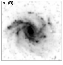
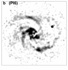
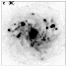
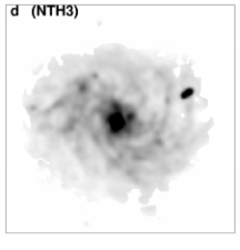
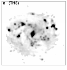
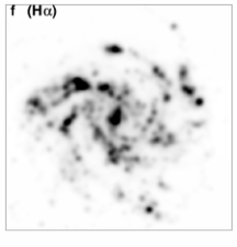
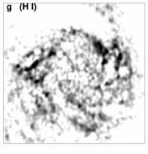
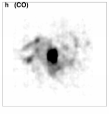
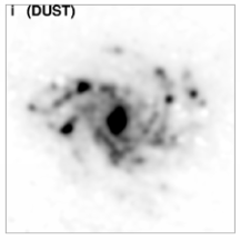
Figure 4: Images of NGC 6946 in different spectral ranges. Top row (from left to right): a optical (red) light, b linearly polarised radio continuum emission at $\lambda$6.2 cm, c total radio continuum emission at $\lambda$6.2 cm. Middle row: d nonthermal radio continuum emission at $\lambda$3.5 cm, e thermal radio continuum emission at $\lambda$3.5 cm, f H$\alpha$ line emission of ionised hydrogen ${\rm H\,\scriptstyle II}$. Bottom row: g line emission of neutral atomic hydrogen ${\rm H\,\scriptstyle I}$, h (1-0) line emission of the CO molecule, i mid-infrared emission of warm dust and PAH particles at 12–18 $\mu$m. The size of every image is $11\arcmin\times 11\arcmin$ and the beam diameter is always $15\arcsec$.

NGC 6946 is a nearby spiral galaxy for which a distance of 5.5 Mpc is usually assumed. Data in many spectral ranges are available. For our analysis we used:

a) The map of the optical broadband emission in red light (R) from the digitized Palomar Sky Survey. We subtracted foreground stars from the map and smoothed it to the angular resolution of the radio continuum maps. The result is shown in Fig. 2.

b) The map of the linearly polarised radio continuum emission at $\lambda$6.2 cm (PI6), combined from observations with the VLA synthesis telescope operated by the NRAO and the Effelsberg single dish operated by the MPIfR (Beck & Hoernes 1996). The angular resolution is $15\arcsec$ which corresponds to 400 pc at the assumed distance to NGC 6946 (5.5 Mpc).

c) The map of the total radio continuum emission at $\lambda$6.2 cm (I6), combined from observations with the VLA synthesis telescope and the Effelsberg single dish (Beck & Hoernes 1996). The angular resolution is $15\arcsec$. We subtracted a strong unresolved source on the northwestern edge of NGC 6946 because it seems unrelated to the galaxy.

d) The map of the nonthermal (synchrotron) radio continuum emission at $\lambda$3.5 cm (NTH3), derived from the spectral index map between $\lambda$3.5 cm and $\lambda$20.5 cm at $15\arcsec$ resolution (Beck, in prep.) assuming a constant synchrotron spectral index of $\alpha=-0.9$ (where the flux density $S$ varies with frequency $\nu$ as $S_{\nu}\propto\nu^{\alpha}$). The spectral index and nonthermal intensity were computed only for pixels where both intensity values exceed 10 times the rms noise.

e) The map of the thermal radio continuum emission (free-free emission from ionised hydrogen) at $\lambda$3.5 cm (TH3) which is the difference map between the total and the synchrotron emission.

f) The map of the H$\alpha$ line emission (H$\alpha$) of ionised hydrogen ${\rm H\,\scriptstyle II}$, integrated over the whole frequency width of the line (Ferguson et al. 1998). We subtracted foreground stars and smoothed the map to the angular resolution of the radio continuum maps. The H$\alpha$ map by Ferguson et al. (1998) has a higher signal-to-noise ratio than the map used in Frick et al. (2000).

g) The map of the radio line emission of neutral atomic hydrogen ${\rm H\,\scriptstyle I}$ at $\lambda$21.1 cm (${\rm H\,\scriptstyle I}$) observed with the Westerbork Synthesis Radio Telescope, integrated over the whole frequency width of the line (Kamphuis & Sancisi 1993). The ${\rm H\,\scriptstyle I}$ map has an original resolution of $13\arcsec\times 16\arcsec$ and was not smoothed.

h) The map of the (1-0) line emission of the molecule CO at $\lambda 2.6$ mm (CO) observed with the IRAM 30-m single-dish telescope, integrated over the whole frequency width of the line (Walsh et al. 2001). The CO map has an original resolution of $22\arcsec$ and was not smoothed. The lower resolution of the CO map compared with the other maps may influence the comparison on small scales, but the effect turns out to be small (see Fig. 10).

i) The map of the mid-infrared emission (12–18 $\mu$m) (DUST) observed with the ISOCAM camera (filter LW3) on board of the ISO satellite (Dale et al. 2000). This wavelength range is dominated by the band of emission lines from polycyclic aromatic hydrocarbons (PAHs) at 12.7 $\mu$m, but also includes continuum emission from small, warm dust grains. The LW3 map has an original resolution of about $8\arcsec$ and was smoothed to a beamwidth of $15\arcsec$.

The map in LW2 (5–8.5 $\mu$m) is fully dominated by PAH emission bands. As it is very similar to the LW3 map, we did not include it in our analysis.

All maps were transformed to the same area ($11\arcmin\times 11\arcmin$) and pixel size ($2\arcsec$). Each map contains $331\times 331$ pixels. Plots of these images are shown in Fig. 4.

In the radio continuum maps, we removed the bright double source at the western edge of the galaxy which has no counterpart in any other spectral range and thus is most probably unrelated to NGC 6946. Finally, we removed the central region in 7 of the 9 maps by subtracting fitted Gaussian sources with half-power widths of about $0\aas@@fstack{\prime}3$ (infrared, total, nonthermal and thermal radio), $0\aas@@fstack{\prime}5$ (H$\alpha$, CO) and $1\arcmin$ (red light). This avoids artefacts produced by improper continuum background subtraction in the central region of the H$\alpha$ map as well as contamination of the mid-infrared map by enhanced continuum emission from warm dust grains.

5.2 Spectral characteristics

Before starting the presentation of spectral characteristics of maps of an external galaxy we want to emphasize that one should be very careful when interpreting such kind of results for two reasons. Firstly, for the scales that are reliably resolved, the maps cannot be treated as homogeneous and isotropically turbulent (as is possible when analysing the Milky Way turbulence from Galactic surveys (Minter & Spangler 1996)). One can expect to find the dominant scale in the map at a certain wavelength (if it exists) and the scale below which the field under consideration can be interpreted as homogeneous – that is one may separate the large-scale structures and the small-scale turbulence. Secondly, one has to carefully separate the spectral properties of the analysed image from the spectral properties of the analysing function and from structures caused by observational problems (regions without observations, bright sources, instrumental noise etc).

We first show the spectral characteristics as defined above for two maps of NGC 6946: the total radio emission (Fig. 5) and the distribution of the H$\alpha$ emission (Fig. 6). Clearly, the structure function totally smoothes the spectral energy distribution suggesting a spectrum of fully developed turbulence on all scales with a power law of slope 0.7. However, the other curves show that such a spectrum is not present in the data. The Fourier spectrum clearly displays the border between the informative part of the spectrum and the small-scale noise, visible as a flat (or even increasing, as in the H$\alpha$ spectrum) part for scales smaller than 0$\aas@@fstack{\prime}$2. This scale is close to the size of the beam (0$\aas@@fstack{\prime}$25) and proves the evident statement that little can be said about scales below the scale of the beamwidth. The structure function and the wavelet spectra show less flattening on scales smaller than the beam.

Figure 5: NGC 6946. Spectral characteristics of the map of total radio emission (I6): second-order structure function (crosses), MH wavelet spectrum (dots), PH wavelet spectrum (circles), Fourier spectrum (line). The size of a pixel is $0\aas@@fstack{\prime}03$ and the beam diameter is $0\aas@@fstack{\prime}25$.

Figure 6: NGC 6946. Spectral characteristics of the H$\alpha$ map: second-order structure function (crosses), MH wavelet spectrum (dots), PH wavelet spectrum (circles), Fourier spectrum (line). The size of a pixel is $0\aas@@fstack{\prime}03$ and the beam diameter is $0\aas@@fstack{\prime}25$.

Wavelet spectra again give an intermediate presentation of the spectral properties. As the optimal spectral characteristic the PH wavelet spectrum can be proposed which smoothes the numerous peaks in the Fourier decomposition but is still sensitive enough to indicate the scales containing most of the energy. The I6 spectrum shows two weak maxima at 0$\aas@@fstack{\prime}$5 and 1$\aas@@fstack{\prime}$3. Note that the spectrum obtained by the MH wavelet does not separate these two maxima. The wavelet spectrum of H$\alpha$ shows a well pronounced maximum at 0$\aas@@fstack{\prime}$8–1$\aas@@fstack{\prime}$0. Even this maximum is hardly visible in the structure function.

In Fig. 7 we present wavelet spectra calculated for all 9 images of NGC 6946 using the PH wavelet (6). The range of scales is limited to $0\aas@@fstack{\prime}2<a<4\aas@@fstack{\prime}0$. Comparing the spectral distributions we note that only H$\alpha$ and TH3 show a clear maximum (though shifted in scale, see Sect. 6.1). Less strong maxima are visible in CO, ${\rm H\,\scriptstyle I}$, R and nonthermal emission NTH3. Almost flat are the spectra of total radio emission I6 and polarised radio emission PI6 – they both show weak maxima near 0$\aas@@fstack{\prime}$5 and 1$\aas@@fstack{\prime}$2. The location of the maxima differs for the images. The thermal emission TH3 and ${\rm H\,\scriptstyle I}$ contain most of the energy on the scale of about 0$\aas@@fstack{\prime}$5, CO on 0$\aas@@fstack{\prime}$7, H$\alpha$ and R on 1$\aas@@fstack{\prime}$0, the NTH3 (and maybe I6) on 1$\aas@@fstack{\prime}$4–1$\aas@@fstack{\prime}$5. For comparison: the typical size of a giant complex of gas clouds is $\approx 1$ kpc (0$\aas@@fstack{\prime}$6), the typical width of the spiral arms is $\approx 1.5$ kpc (0$\aas@@fstack{\prime}$9).

The spectra in Fig. 7 show that the spatial resolution of the available images is insufficient for the study of properties of the small-scale turbulence. The inertial range is expected to start at scales several times smaller than the dominant scale (turbulent macroscale). If the observed object contains the classical three-dimensional Kolmogorov turbulence with the spectrum $E(k)\sim k^{-5/3}$ (corresponding to the structure function $S_{2}\sim l^{2/3}$), the two-dimensional projection should be characterized be a structure function $S_{2}\sim l^{5/3}$ (Spangler 1991). The spectral slope of the projected field steepens because the smaller scales are smoothed in the projection. In Fig. 7, only TH3 and H$\alpha$ show Kolmogorov-type behaviour on small scales (see Sect. 6.1).

Figure 7: NGC 6946. Wavelet spectra (analysing wavelet is PH). The thin lines above H$\alpha$ and TH3 indicate a slope of 5/3.

Figure 8: NGC 6946. Scale-by-scale wavelet cross-correlations: H$\alpha$–PI6 (dots); H$\alpha$–TH3 (stars); H$\alpha$–NTH3 (circles).

5.3 Cross-correlations in the galaxy NGC 6946

We start by calculating the classical “pixel by pixel” cross-correlation coefficient $r_{p}$ for every pair of galactic maps under discussion. The values of $r_{p}$ are given in the upper part (above the diagonal) of Table 1. Note that for most pairs the value of the coefficient indicates a statistically significant correlation. Only the PI6 map in pair with TH3, H$\alpha$ and ${\rm H\,\scriptstyle I}$ yields correlation coefficients significantly less than 0.5 (0.23, 0.25 and 0.29, respectively).

Table 1: Cross-correlations between 9 maps of NGC 6946. The classical correlation coefficients $r_{p}$ are given above the diagonal of the table. Below the diagonal the mean values of the wavelet correlation coefficient $r_{w}(a)$, calculated for the range of scales $0\aas@@fstack{\prime}4<a<1\aas@@fstack{\prime}2$, are shown.

	R	PI6	I6	NTH3	TH3	H$\alpha$	${\rm H\,\scriptstyle I}$	CO	DUST
R		$0.51$	$0.84$	$0.86$	$0.66$	$0.77$	$0.44$	$0.83$	$0.88$
		$\pm 0.03$	$\pm 0.02$	$\pm 0.02$	$\pm 0.03$	$\pm 0.02$	$\pm 0.03$	$\pm 0.02$	$\pm 0.02$
PI6	$-0.11$		$0.56$	$0.67$	$0.23$	$0.25$	$0.29$	$0.53$	$0.49$
	$\pm 0.06$		$\pm 0.03$	$\pm 0.03$	$\pm 0.03$	$\pm 0.03$	$\pm 0.03$	$\pm 0.03$	$\pm 0.03$
I6	$0.49$	$0.19$		$0.92$	$0.81$	$0.77$	$0.47$	$0.78$	${\mathbf{0}.94}$
	$\pm 0.05$	$\pm 0.06$		$\pm 0.02$	$\pm 0.02$	$\pm 0.02$	$\pm 0.03$	$\pm 0.02$	${\mathbf{\pm}0.02}$
NTH3	$0.29$	$0.36$	$0.71$		$0.60$	$0.64$	$0.40$	$0.80$	$0.89$
	$\pm 0.06$	$\pm 0.06$	$\pm 0.04$		$\pm 0.03$	$\pm 0.03$	$\pm 0.03$	$\pm 0.02$	$\pm 0.02$
TH3	$0.57$	$-0.10$	$0.77$	$0.53$		$0.81$	$0.45$	$0.57$	$0.79$
	$\pm 0.05$	$\pm 0.06$	$\pm 0.04$	$\pm 0.05$		$\pm 0.02$	$\pm 0.03$	$\pm 0.03$	$\pm 0.02$
H$\alpha$	$0.68$	$-0.22$	$0.65$	$0.34$	$0.80$		$0.50$	$0.65$	$0.81$
	$\pm 0.05$	$\pm 0.06$	$\pm 0.05$	$\pm 0.06$	$\pm 0.03$		$\pm 0.03$	$\pm 0.03$	$\pm 0.02$
${\rm H\,\scriptstyle I}$	$0.35$	$0.14$	$0.47$	$0.39$	$0.37$	$0.41$		$0.41$	$0.43$
	$\pm 0.06$	$\pm 0.06$	$\pm 0.06$	$\pm 0.06$	$\pm 0.06$	$\pm 0.06$		$\pm 0.03$	$\pm 0.03$
CO	$0.35$	$0.24$	$0.48$	$0.32$	$0.36$	$0.36$	$0.49$		$0.85$
	$\pm 0.06$	$\pm 0.06$	$\pm 0.06$	$\pm 0.06$	$\pm 0.06$	$\pm 0.06$	$\pm 0.06$		$\pm 0.02$
DUST	$0.56$	$0.14$	${\mathbf{0}.84}$	$0.47$	$0.63$	$0.60$	$0.57$	$0.66$
	$\pm 0.05$	$\pm 0.06$	${\mathbf{\pm}0.04}$	$\pm 0.06$	$\pm 0.05$	$\pm 0.05$	$\pm 0.05$	$\pm 0.05$

For each pair of maps the wavelet correlation coefficient $r_{w}$ was also calculated, using the MH wavelet. As an example, the behaviour of $r_{w}(a)$ is shown in Fig. 8 for three pairs of data: H$\alpha$–PI6, H$\alpha$–TH3 and H$\alpha$–NTH3. The high correlation on largest scales reflects only the coincidence of the extended regions corresponding to the galaxy’s disk (see Fig. 2, bottom right). However, on intermediate scales the three curves display very different behaviours. The anticorrelation between H$\alpha$ and PI6 is of special interest (see Sect. 6.2). The tendency of all curves in Fig. 8 to grow towards the smallest scale ($a=0\aas@@fstack{\prime}125$) indicates that this scale is affected by fluctuations on scales significantly smaller than the resolution of the maps ($0\aas@@fstack{\prime}25$) and thus will not be considered further, whereas the next computed scale ($a=0\aas@@fstack{\prime}2$), though still slightly smaller than the beam size, gives useful information. Note that the number of independent points decreases towards larger scales which results in increasing error bars on these scales.

Figure 9: NGC 6946. Cross-correlations of the intensities of the initial images and of their wavelet decompositions. Polarised radio emission (PI6) versus H$\alpha$: a initial data, b wavelet coefficients $w$ for scales $a=1\arcmin$, c for $a=2\aas@@fstack{\prime}8$. Thermal radio emission (TH3) versus H$\alpha$: d initial data, e wavelet coefficients $w$ for scales $a=1\arcmin$, f for $a=2\aas@@fstack{\prime}8$.

To illustrate the difference in correlating the initial data and the wavelet decomposition on various scales, we show the corresponding plots in Fig. 9 for two extreme cases of Fig. 8. The correlation of the maps PI6 and H$\alpha$ gives $r_{p}=0.25$. This low value of $r_{p}$ is understandable when looking at the distribution of points in Fig. 9a. In panel (b) we show the wavelet coefficients $W(a,\vec{x})$ obtained for the PI6 map versus the corresponding wavelet coefficients calculated for the H$\alpha$ map. The scale parameter is fixed at the value $a=1\aas@@fstack{\prime}0$, which corresponds to the minimum in the curve $r_{w}(a)$ for this pair of maps in Fig. 8. The cloud of points becomes elongated along the line $y=-x$ which corresponds to a negative value of $r_{w}$. Note that the wavelet coefficients $W(a,\vec{x})$ become negative in case of local minima on a certain scale in the analysed data. Panel (c) shows the corresponding plot for the same pair of maps, but for the scale $a=2\aas@@fstack{\prime}8$, which gives $r_{w}=0.57$. The tendency of a positive correlation becomes visible.

Panels (d), (e) and (f) of Fig. 9 present the analogous plots for the maps TH3 and H$\alpha$. This pair of data shows a high degree of correlation: $r_{p}=0.81$. Note that the plot in panel (e) corresponding to $W(a,\vec{x})$ at $a=1\aas@@fstack{\prime}0$ (a local maximum in $r_{w}(a)$, see Fig. 8) gives a better confined cloud of points than the initial data in panel (d), in spite of the fact that the correlation coefficient is $r_{w}=0.71$ (less than $r_{p}$). This means that the scatter in the points in panel (d) is compensated by the larger number of points along the central strip of the cloud. The points in panel (e) are also more homogeneously distributed than in panel (d). Panel (f) shows again the scale $a=2\aas@@fstack{\prime}8$, on which TH3 and H$\alpha$ are less correlated than on the scale $a=1\aas@@fstack{\prime}0$ ($\simeq 1.6$ kpc, the typical width of a spiral arm).

When analysing galactic images, the scales which characterize the width of the spiral arms are of special interest. Therefore we calculated the mean value of $r_{w}$ for the range of scales $0\aas@@fstack{\prime}4<a<1\aas@@fstack{\prime}2$. These scales are also more certain in the sense that they are large enough with respect to the size of the beam and small enough to give satisfactory statistics over the area of the galactic image. The values derived are given in the lower part of the Table 1 (below the diagonal).

Comparing the corresponding values of $r_{p}$ and $r_{w}$ in Table 1, three groups of map pairs can be distinguished: 1) the two correlation coefficients are similar (the difference between $r_{p}$ and $r_{w}$ is less than 25%), 2) the two correlation coefficients strongly differ, $r_{p}/r_{w}\approx 2$ or even $r_{w}<0$ ($r_{p}$ is never negative in the table), 3) comme ci - comme ça.

Group 1 includes most of the pairs containing ${\rm H\,\scriptstyle I}$ or TH3 (only the pairs ${\rm H\,\scriptstyle I}$–PI6, TH3–PI6 strongly drop out of this rule) and several pairs with H$\alpha$: H$\alpha$–R, H$\alpha$–I, H$\alpha$–DUST. The coefficients $r_{p}$ and $r_{w}$ are practically equal for ${\rm H\,\scriptstyle I}$–I6, ${\rm H\,\scriptstyle I}$–NTH3, TH3–H$\alpha$, and TH3–I6. In the whole table only the pairs ${\rm H\,\scriptstyle I}$–CO and ${\rm H\,\scriptstyle I}$–DUST give $r_{w}>r_{p}$.

Group 2 includes first of all the correlations with PI6. Three pairs (PI6–R, PI6–TH3, PI6–H$\alpha$) yield negative $r_{w}$. Strong differences between $r_{w}$ and $r_{p}$ occur in R–NTH3 (0.29/0.86), R–CO (0.35/0.83), NTH3–CO (0.32/0.80), NTH3–H$\alpha$ (0.34/0.64), and NTH3-DUST (0.47/0.89).

We calculated 36 cross-correlation functions $r_{w}(a)$, one for each pair of galactic maps. Because of space limitation we present the correlation curves $r_{w}(a)$ only for two sets of pairs (see Fig. 10: red emission R (left column) and polarised emission PI6 (right column) correlated with each of the other 8 maps.

Figure 10: NGC 6946. Wavelet cross-correlations for red light (R, left) and polarised radio emission (PI6, right) versus each of the other maps.

For most pairs $r_{w}$ varies considerably with scale. Only a few curves display a weak dependence on scale, for example R–DUST, which leads to similar values for $r_{w}$ and $r_{p}$ (Group 1). The best coincidence of $r_{w}$ and $r_{p}$, however, is obtained when $r_{w}$ has a maximum on the scales chosen for the calculation of $r_{w}$ for Table 1. The pairs R–${\rm H\,\scriptstyle I}$ (see Fig. 10) and H$\alpha$–TH3 (Fig. 8) are good examples of this case. Also the pairs ${\rm H\,\scriptstyle I}$–CO, H$\alpha$–I6, TH3–DUST show well pronounced local maxima on the scale of the arm width.

Obviously, the main part of Group 2 (high contrast between $r_{p}$ and $r_{w}$) consists of pairs for which the $r_{w}$ curve has a minimum on intermediate scales. Apart from all pairs including PI6, the pairs CO–NTH and CO–R belong to this group. In these cases the classical cross-correlation coefficient can be misleading (see Sect. 6.2).

6 Conclusions and Discussion

In this paper we have used the wavelet analysis to find the scales of dominant structures in maps of the spiral galaxy NGC 6946 observed in various spectral ranges and to study cross-correlation coefficients between pairs of maps. Our conclusions are summarised below.

6.1 Wavelet spectra

We would like to stress once again that the scaling analysis of observational data requires an adequate choice of the mathematical tool. We have shown that the structure function, which is a commonly used method for scaling analysis of small-scale turbulence, is not suitable for scales which are close to the dominating large-scale structures (see Figs. 5 and 6). Due to poor scale resolution, the structure function may suggest that a continuous range of scales with a power law exists (as e.g. in Beck et al. 1999) even when this is not present in the data. On the contrary, the traditional Fourier technique applied to real data gives very spiky spectra in which the separation of real maxima and high harmonics can be difficult.

We have shown that wavelets (provided the choice of the wavelet is adequate to the aim of the analysis and to the analysed data) allow to obtain reliable spectral characteristics of the object even if the range of scales in the map is relatively small (about one and a half decades in our cases). A suitable choice of wavelets leads to smooth spectra which clearly indicate the dominant scales in the analysed data.

Using wavelets, the spectral characteristics of 9 optical, radio and infrared maps of the galaxy NGC 6946 were calculated. The wavelet spectra in Fig. 7 show three types of curves:

a) R, I6, CO and DUST increase smoothly with increasing scale. These maps show structures on small and large scales (clouds, spiral arms, an extended central region and extended diffuse emission).

b) The spectrum of PI6 is practically flat on all scales because this map neither contains an extended central region nor extended diffuse emission.

c) TH3 and H$\alpha$ show a prominent maximum on intermediate scales corresponding to the width of the spiral arms. The maximum in TH3 occurs on a somewhat smaller scale than that in H$\alpha$. A possible explanation is the increase of absorption of the H$\alpha$ emission on small scales where gas densities are generally higher (see also Fig. 12).

We conclude that the wavelet spectrum reveals signatures of different phenomena in an object and allows to compare their relative importance within the object as well as between different objects or wavelength ranges.

Only two spectra, H$\alpha$ and thermal emission TH3, include an increasing part on small scales, which (with great caution) can be interpreted as an indication of the Kolmogorov inertial range in which the energy is transferred from large to small scales. In Fig. 7 we show the expected theoretical slope of 5/3 as thin lines at $a<0\aas@@fstack{\prime}5$ (800 pc) for H$\alpha$ and at $a<0\aas@@fstack{\prime}35$ (560 pc) for TH3. We also analysed the spectrum of the H$\alpha$ image at full resolution ($\simeq 2\arcsec$) and found that the slope of 5/3 continues down to a scale of about $0\aas@@fstack{\prime}1$ (160 pc). Note that this slope should characterize the two-dimensional projection of a three-dimensional turbulent field with Kolmogorov spectral properties.

Some spectra in Fig. 7 include an increasing part with a slope of less than 1. Red light R shows a slope $\approx 0.6$ for $0\aas@@fstack{\prime}25\leq a\leq 1\arcmin$, in CO the slope is close to $0.7$ for $0\aas@@fstack{\prime}25\leq a<1\arcmin$, and in the same range of scales the DUST emission is characterized by a slope $\approx 0.5$. The total radio emission I6 shows a large range of scales with growing energy, but the slope is not constant and depends on the choice of the range; a weak maximum near $a=0\aas@@fstack{\prime}5$ may indicate two subintervals with different slopes. The mean slope in the range $0\aas@@fstack{\prime}25\leq a\leq 1\aas@@fstack{\prime}4$ is about 0.6–0.7.

Structure functions with a slope of about 2/3 over a range of scales have been interpreted as an indication of two-dimensional turbulence (Minter & Spangler 1996; Beck et al. 1999). This interpretation, however, is uncertain because the physical behaviour of two-dimensional turbulence is quite different from three-dimensional turbulence.

In 2-D turbulence two inertial ranges are possible (Kraichnan 1967). This is due to an additional conservation law, i.e. in the limit of small viscosity the total square of vorticity, called enstrophy, becomes an integral of motion as well as the total energy. The first inertial range, the range of inertial transport of enstrophy to smaller scales, appears on scales smaller than the scale where the turbulence is excited. The dimensional arguments lead to a very steep spectrum $E(k)\sim k^{-3}$, which corresponds to a structure function $S_{2}\sim l^{2}$. No average spectral flux of energy is expected in this inertial range. The second inertial range can appear on scales larger than the scales on which the energy input into the flow occurs. Although characterized by the usual Kolmogorov spectral slope ($E(k)\sim k^{-5/3}$ or $S_{2}\sim l^{2/3}$), it has very different physical properties because the energy in this inertial range can be transferred only to larger scales (so-called inverse energy cascade). It is important to note that the formation of the inverse energy cascade is a relatively slow process and implies a stationary forcing on intermediate scales (see, e.g., Borue (1994) or Babiano, Dubrulle & Frick (1997)). Two-dimensional turbulence with a slope of 2/3 implies the existence of an inertial range of scales with inverse cascade. This means that the energy of turbulent motion on these scales does not emerge from the larger (galactic) scale, but is transferred from smaller (sub-galactic) scales on which nevertheless the motion already has to be two-dimensional, which is improbable.

At the moment we cannot explain the origin of the slopes of about 2/3 detected in the wavelet spectrum of R, CO, DUST and I6 on small scales. Furthermore, we do not understand why a slope of about 5/3 is observed only for the ionised gas (H$\alpha$ and TH3). Future images with higher resolution are needed in order to extend the analysis to smaller scales.

6.2 Cross-correlations

We have introduced a new cross-correlation characteristic based on wavelet decomposition, named the wavelet cross-correlation, which allows to analyse the correlation as a function of scale. The classical cross-correlation coefficient is misleading if a bright, extended central region or an extended disk exists in the galactic images. In such cases (see R, I6, NTH3, CO and DUST in Table 1) the classical cross-correlation is dominated by the large-scale structure which can be identified as the galaxy’s disk with its general radial decrease in intensity (see Fig. 2, bottom right), while the (more interesting) correlation on scales of the spiral arms can be much worse. In Table 1 this is clearly indicated by the wavelet correlation coefficients $r_{w}$ which are much lower than the corresponding values of the classical coefficient $r_{p}$.

In classical cross-correlation analysis, the general radial decrease of a galaxy’s intensity can be removed by dividing all values within a certain radial range by its mean (see e.g. Hoernes et al. 1998). This is similar to removing the largest scale from a map only if the radial decrease is smooth and independent of azimuthal angle. The wavelet technique is recommended as the more reliable method.

Figure 11: NGC 6946. Wavelet cross-correlations for mid-infrared dust emission (DUST) versus total (I6), nonthermal (NTH3) and thermal (TH3) radio emission.

The best correlation, with $r_{w}>0.75$ for any scale $a$, yields the pair DUST–I6 (Fig. 11). The correlation between DUST and each of the two components of radio continuum, nonthermal and thermal emission, is significantly worse. This indicates that the correlation between the total intensities is not due to a single process like star-formation activity or coupling of magnetic fields to gas clouds, but needs a cooperation of physical processes on all scales. A detailed analysis will be the subject of a separate paper.

Similarly, the far-infrared emission of the total dust in M31 is highly correlated with the total radio emission, while the correlations between the components warm dust – thermal radio and between cool dust – nonthermal radio are worse (Hoernes et al. 1998; Berkhuijsen, Nieten & Haas 2000).

We have shown that the anticorrelation between PI6 and TH3 (and between PI6 and H$\alpha$) can be quantified using wavelet analysis. This phenomenon, which is due to the phase shift between the magnetic arms and the optical arms (Beck & Hoernes 1996; Frick et al. 2000), exists only on intermediate scales and is clearly visible as a minimum in Fig. 8 (lower curve) and Fig. 10 (right). The position of this minimum indicates the scale on which the anticorrelation is strongest, i.e. $\simeq 1\aas@@fstack{\prime}0$ or 1.6 kpc at the distance of NGC 6946, which is the typical width of a spiral arm.

The absolute value of the wavelet correlation coefficient in these minima is relatively small (0.1–0.25 only). This fact can be explained twofold. Firstly, the structures which are responsible for this anticorrelation (the arms) occupy only a limited part of the image. Secondly, in contrast to the illustrative example given in Fig. 3, real arms are more irregular in space and in scales. This is why the position of the local extremum in the correlation curve $r_{w}(a)$ can be informative even if the absolute value of $r_{w}(a)$ is relatively small.

Figure 12: NGC 6946. Wavelet cross-correlation between H$\alpha$ and thermal radio continuum emission (TH3).

Fig. 12 shows the correlation between the two tracers of ionised gas. The correlation is high on intermediate and large scales, but relatively low on small scales. This gives further indication for enhanced absorption of the H$\alpha$ emission on small scales. Thus wavelet analysis can be used to study the distribution of the absorbing dust.

Future radio images with better resolution will allow to study the correlation on smaller scales.

References

- [1] Aurell E., Frick P., Shaidurov V., 1994, Physica D, 72, 95
- [2] Babiano A., Dubrulle B., Frick P., 1997, Phys. Rev. E, 55, 2693
- [3] Beck R., 2001, in Diehl R., Kallenbach R., Parizot E., von Steiger R., eds., The Astrophysics of Galactic Cosmic Rays. Space Science Rev., Kluwer, Dordrecht, in press (astro-ph 0012402)
- [4] Beck R., Hoernes P., 1996, Nature, 379, 47
- [5] Beck R., Berkhuijsen E.M., Uyanıker B., 1999, in Ostrowski M., Schlickeiser R., eds., Plasma Turbulence and Energetic Particles in Astrophysics. Jagiellonski University, Krakow, p. 5
- [6] Berkhuijsen E.M., Bajaja E., Beck R., 1993, A&A, 279, 359
- [7] Berkhuijsen E.M., Nieten C., Haas M., 2000, in Berkhuijsen E.M., Beck R., Walterbos R.A.M., eds., The Interstellar Medium in M31 and M33, Shaker Verlag, Aachen, p. 187
- [8] Borue V., 1994, Phys. Rev. Lett., 72, 1475
- [9] Chen P.C., Zhang X.Z., Xiang S.P., Feng L.L., Reich W., 2000, Chin. Phys. Lett., 17, 388
- [10] Dale D.A. et al., 2000, AJ, 120, 583
- [11] Edwards A.L., 1979, Multiple Regression and Analysis of Variance and Covariance. W.H. Freeman and Company, San Francisco
- [12] Elmegreen B.G., Elmegreen D.M., Montenegro L., 1992, ApJS, 79, 37
- [13] Ferguson A.M.N., Wyse R.F.G., Gallagher J.S., Hunter D.A., 1998, ApJ, 506, L19
- [14] Foster G., 1996, AJ, 112, 1709
- [15] Frick P., Baliunas S.L., Galyagin D., Sokoloff D., Soon W., 1997a, ApJ, 483, 426
- [16] Frick P., Galyagin D., Hoyt D., Nesme-Ribes E., Shatten K., Sokoloff D., Zakharov V., 1997b, A&A, 328, 670
- [17] Frick P., Beck R., Shukurov A., Sokoloff D., Ehle M., Kamphuis J., 2000, MNRAS, 318, 925
- [18] Frisch U., 1995, Turbulence. Cambridge University Press, Cambridge
- [19] Hoernes P., Berkhuijsen E.M., Xu C., 1998, A&A, 334, 57
- [20] Holschneider M., 1995, Wavelets: An Analysis Tool. Oxford University Press, Oxford
- [21] Kamphuis J., Sancisi R., 1993, A&A, 273, L31
- [22] Kraichnan R., 1967, Phys. Fluids, 10, 1417
- [23] Minter A.H., Spangler S.R., 1996, ApJ, 458, 194
- [24] Monin A.S., Yaglom A.M., 1971, in Lumley J., ed., Statistical Fluid Mechanics, Vol. 1. MIT Press, Cambridge, MA
- [25] Monin A.S., Yaglom A.M., 1975, in Lumley J., ed., Statistical Fluid Mechanics, Vol. 2. MIT Press, Cambridge, MA
- [26] Nesme-Ribes E., Frick P., Sokoloff D., Zakharov V., Ribes J.-C., Vigouroux A., Laclare F., 1995, C. R. Acad. Sci. Paris, 321, IIb, 525
- [27] Rohde R., Beck R., Elstner D., 1999, A&A, 350, 423
- [28] Spangler S.R., 1991, ApJ, 376, 540
- [29] Spangler S.R., 1999, in Ostrowski M., Schlickeiser R., eds., Plasma Turbulence and Energetic Particles in Astrophysics. Jagiellonski University, Krakow, p. 1
- [30] Tenorio L., Jaffe A.H., Hanany S., Lineweaver C.H., 1999, MNRAS, 310, 823
- [31] Torresani B., 1995, Continuous Wavelet Transform. Savoire, Paris
- [32] Walsh W., Thuma G., Beck R., Weiss A., Wielebinski R., Dumke M., 2001, A&A, submitted