An Efficient Monte Carlo Algorithm for a
Restricted Class of Scattering Problems
in Radiation Transfer

Se describe un algoritmo eficiente tipo Monte Carlo para solucionar una clase restringida de problemas en la transferencia de radiación. Esta clase incluye varios problemas de interés en la astrofísica, incluyendo la dispersión de la luz ultravioleta y visible por granos. El algoritmo toma en cuenta la dispersión múltiple. Se describe el algoritmo, se presentan algunas optimizaciones importantes, y se muestra explícitamente cómo se puede usar el algoritmo para estimar cantidades como la intensidad emergente y promedio. Se presenta dos pruebas del algoritmo, se examina la importancia de las optimizaciones, y se muestra que el algoritmo se puede aplicar de manera útil a los problemas ópticamente delgados, los cuales son a veces considerados limitados a aproximaciones explícitas de dispersión sencilla más atenuación.

Abstract

We describe an efficient Monte Carlo algorithm for a restricted class of scattering problems in radiation transfer. This class includes many astrophysically interesting problems, including the scattering of ultraviolet and visible light by grains. The algorithm correctly accounts for multiply-scattered light. We describe the algorithm, present a number of important optimizations, and explicity show how the algorithm can be used to estimate quantities such as the emergent and mean intensity. We present two test cases, examine the importance of the optimizations, and show that this algorithm can be usefully applied to optically-thin problems, a regime sometimes considered limited to explicit single-scattering plus attenuation approximations.

0.1 Introduction

We present a Monte Carlo algorithm for the numerical solution of a restricted class of scattering problems in radiation transfer. This class consists of problems in which the true emissivity (the emissivity of unscattered light) and the opacity, albedo, and scattering properties are specified a priori and are zero outside a finite domain, but have arbitrary distributions within that finite domain. In particular, no restrictions are placed on the scattering phase function or on the symmetry of the problem. Examples of problems that satisfy these requirements include those in which the opacity is dominated some combination of grain opacity, electron scattering, resonance-line scattering, Rayleigh scattering, or Raman scattering. For example, the transfer of ultraviolet and visible light in the presence of grains and of Ly$\alpha$ photons in the presence of neutral hydrogen and grains. For simplicity, in this paper we do not consider time-dependent problems or polarization, however, as we discuss in §0.8, the algorithm can be easily extended to cover these cases.

We have developed this algorithm over the last several years, initially independently (Watson 1994; Henney 1994ab; Henney 1995; Henney & Axon 1995; Burrows et al. 1996; Sahai et al. 1998; and Henney 1998) and then collaboratively (Stapelfeldt et al. 1999; Watson et al. 2001). The algorithm currently incorporates several important features and optimizations, including the use of forced scatterings and forced interactions, the construction of estimators from unbiased samples of scattering events, and a very efficient integrator for optical depth.

Monte Carlo algorithms have been widely used in radiation transfer (see §0.3). It seems clear to us that aspects of this algorithm have been independently discovered and appear to be common knowledge among those working in this field. The principal contribution of this paper is to formalize and publish the algorithm, so that it can be better understood and so that future researchers can avoid the wasted effort of independent rediscovery.

In §2 we present the restricted problem along with a formal (but computationally intractable) solution. In §3 we briefly discuss previous approaches to this problem. In §4 we present the algorithm and a number of optimizations and variations. In §5 we discuss important details of our implementations. In §6 we present two test cases. In §7 we quantify the efficiency gains due to two important optimizations. In §8 we briefly outline how the algorithm might be extended to include time dependence and polarization. In §9 we summarize our main results.

0.2 The Restricted Problem

Table 1: Notation

Symbol	Definition	Units
$\mathbf{r}$	Position.	cm
$\mathbf{r}_{i}$	Position of the $i$-th interaction with matter.	cm
$\mathbf{n}$	Direction; $|\mathbf{n}|\equiv 1$.
$\mathbf{n}_{i}$	Direction after the $i$-th interaction with matter.
$\nu$	Frequency.	Hz
$\nu_{i}$	Frequency after the $i$-th interaction with matter.	Hz
$w$	Statistical weight.
$w_{i}$	Statistical weight after the $i$-th interaction with matter.
$\eta(\mathbf{r},\nu,\mathbf{n})$	Total emissivity; $\sum_{i=0}^{\infty}\eta_{i}(\mathbf{r},\nu,\mathbf{n})$.	$\mathrm{erg\,s^{-1}\,cm^{-3}\,sr^{-1}\,Hz^{-1}}$
$\eta_{i}(\mathbf{r},\nu,\mathbf{n})$	Partial emissivity of light scattered $i$ times.	$\mathrm{erg\,s^{-1}\,cm^{-3}\,sr^{-1}\,Hz^{-1}}$
$I(\mathbf{r},\nu,\mathbf{n})$	Total specific intensity; $\sum_{i=0}^{\infty}I_{i}(\mathbf{r},\nu,\mathbf{n})$.	$\mathrm{erg\,s^{-1}\,cm^{-2}\,sr^{-1}\,Hz^{-1}}$
$I_{i}(\mathbf{r},\nu,\mathbf{n})$	Partial specific intensity of light scattered $i$ times.	$\mathrm{erg\,s^{-1}\,cm^{-2}\,sr^{-1}\,Hz^{-1}}$
$\mathcal{L}(\mathbf{r},\nu,\mathbf{n})$	Total radiative intensity, defined in §0.4.4; $\sum_{i=0}^{\infty}\mathcal{L}_{i}(\mathbf{r},\nu,\mathbf{n})$.	$\mathrm{erg\,s^{-1}\,sr^{-1}\,Hz^{-1}}$
$\mathcal{L}_{i}(\mathbf{r},\nu,\mathbf{n})$	Partial radiative intensity of light scattered $i$ times.	$\mathrm{erg\,s^{-1}\,sr^{-1}\,Hz^{-1}}$
$l$	Length.	cm
$\tau(\mathbf{r},\nu,\mathbf{n};l)$	Optical depth from $\mathbf{r}$ to $\mathbf{r}+l\mathbf{n}$; $\int_{0}^{l}dl^{\prime}\>\chi(\mathbf{r}+l^{\prime}\mathbf{n},\nu,\mathbf{n})$.
$\tau_{\infty}(\mathbf{r},\nu,\mathbf{n})$	Optical depth from $\mathbf{r}$ to infinity; $\lim_{l\rightarrow\infty}\tau(\mathbf{r},\nu,\mathbf{n};l)$.
$\chi(\mathbf{r},\nu,\mathbf{n})$	Linear extinction coefficient; $\kappa+\sigma$	$\mathrm{cm^{-1}}$
$\sigma(\mathbf{r},\nu,\mathbf{n})$	Linear scattering coefficient.	$\mathrm{cm^{-1}}$
$\kappa(\mathbf{r},\nu,\mathbf{n})$	Linear absorption coefficient.	$\mathrm{cm^{-1}}$
$a(\mathbf{r},\nu,\mathbf{n})$	Single-scattering albedo; $\sigma/\chi$.
$\Sigma(\mathbf{r};\nu^{\prime},\mathbf{n}^{\prime};\nu,\mathbf{n})$	Scattering outcome function, defined by equation 1.	$\mathrm{sr^{-1}\,Hz^{-1}}$
$\Phi(\mathbf{r};\nu;\mathbf{n}^{\prime},\mathbf{n})$	Scattering phase function, normalized according to equation 3.	$\mathrm{sr^{-1}}$

The restricted problem requires that $\eta_{0}(\mathbf{r},\nu,\mathbf{n})$, $\chi(\mathbf{r},\nu,\mathbf{n})$, $a(\mathbf{r},\nu,\mathbf{n})$, and $\Sigma(\mathbf{r};\nu^{\prime},\mathbf{n}^{\prime};\nu,\mathbf{n})$ be specified a priori. Table 1 defines our notation, which closely follows that of Mihalas (1978), except for the scattering phase function: we use $\Phi$ instead of $g$ for the phase function, to avoid confusion with the asymmetry parameter of the Henyey-Greenstein phase function, and we normalize the phase function according to equation 3, so the phase function has units of $\mathrm{sr^{-1}}$ and an isotropic phase function has a value of $1/4\pi\leavevmode\nobreak\ \mathrm{sr^{-1}}$ everywhere. Note that the emissivities and specific intensities are per unit solid angle and the extinction, scattering, and absorption coefficients are per unit length. We denote by $x_{i}$ the quantity $x$ when only light scattered $i$ times is considered. For example, $\eta_{0}$ is the emissivity of unscattered light, that is, the true emissivity, and $\eta_{1}$ is the emissivity of singly-scattered light. For convenience, we also introduce the single-scattering albedo $a$ and the scattering outcome function $\Sigma$. The albedo $a$ has its conventional definition as the probability that an interaction with matter results in a scattering rather than an absorption. The scattering outcome function $\Sigma$ is defined by

$$\eta(\mathbf{r},\nu,\mathbf{n})=\eta_{0}(\mathbf{r},\nu,\mathbf{n})+\int_{0}^{\infty}\!\!\!\!d\nu^{\prime}\!\!\int_{4\pi}\!\!\!\!d\Omega^{\prime}\!\!\;\;\sigma(\mathbf{r},\nu^{\prime},\mathbf{n}^{\prime})\Sigma(\mathbf{r};\nu^{\prime},\mathbf{n}^{\prime};\nu,\mathbf{n})I(\mathbf{r},\nu^{\prime},\mathbf{n}^{\prime})$$ (1)

That is, $\Sigma(\mathbf{r};\nu^{\prime},\mathbf{n}^{\prime};\nu,\mathbf{n})$ is the contribution to the emissivity $\eta(\mathbf{r},\nu,\mathbf{n})$ when intensity $I(\mathbf{r},\nu^{\prime},\mathbf{n}^{\prime})$ is scattered. We explicitly separate $\sigma$ and $\Sigma$ to distinguish the probability distribution of scattering events from the probability distribution of the outcomes of those events given that they have occurred.

Scattering does not necessarily conserve energy, but it conserves photons. Considering the specific intensity as being carried by photons of energy $h\nu$, we can identify $\Sigma(\mathbf{r};\nu^{\prime},\mathbf{n}^{\prime};\nu,\mathbf{n})(\nu^{\prime}/\nu)$ as the joint probability distribution that upon scattering a photon with frequency $\nu^{\prime}$ and direction $\mathbf{n}^{\prime}$ becomes a photon with frequency $\nu$ and direction $\mathbf{n}$. Thus, integrating over all initial or final states, we have

$$\int_{0}^{\infty}\!\!\!\!d\nu^{\prime}\!\!\int_{4\pi}\!\!\!\!d\Omega^{\prime}\!\!\;\;\Sigma(\mathbf{r};\nu^{\prime},\mathbf{n}^{\prime};\nu,\mathbf{n})(\nu^{\prime}/\nu)=\int_{0}^{\infty}\!\!\!\!d\nu\!\!\int_{4\pi}\!\!\!\!d\Omega\!\!\;\;\Sigma(\mathbf{r};\nu^{\prime},\mathbf{n}^{\prime};\nu,\mathbf{n})(\nu^{\prime}/\nu)\equiv 1,$$ (2)

for any $\nu$ and $\mathbf{n}$ or $\mathbf{n}^{\prime}$ and $\mathbf{n}^{\prime}$. As an example of $\Sigma$, consider coherent scattering ($\nu^{\prime}=\nu$) with a phase function $\Phi(\mathbf{r};\nu;\mathbf{n}^{\prime},\mathbf{n})$ normalized as

$$\int_{4\pi}\!\!\!\!d\Omega^{\prime}\!\!\;\;\Phi(\mathbf{r};\nu;\mathbf{n}^{\prime},\mathbf{n})=\int_{4\pi}\!\!\!\!d\Omega\!\!\;\;\Phi(\mathbf{r};\nu;\mathbf{n}^{\prime},\mathbf{n})\equiv 1;$$ (3)

we then have

$$\Sigma(\mathbf{r};\nu^{\prime},\mathbf{n}^{\prime};\nu,\mathbf{n})(\nu^{\prime}/\nu)=\delta(\nu^{\prime}-\nu)\Phi(\mathbf{r};\nu;\mathbf{n}^{\prime},\mathbf{n}).$$ (4)

The standard formal solution of the equation of radiation transfer gives the intensity $I_{i}(\mathbf{r},\nu,\mathbf{n})$ of photons that have undergone $i$ scatterings as

$$I_{i}(\mathbf{r},\nu,\mathbf{n})=\int_{l=-\infty}^{0}\!\!\!\!\!\!\!\!\!\!dl\!\!\;\;\eta_{i}(\mathbf{r}+l\mathbf{n},\nu,\mathbf{n})e^{-\tau(\mathbf{r},\nu,\mathbf{n};l)},$$ (5)

where

$$\tau(\mathbf{r},\nu,\mathbf{n};l)=\int_{0}^{l}\!\!dl^{\prime}\>\chi(\mathbf{r}+l^{\prime}\mathbf{n},\nu,\mathbf{n}).$$ (6)

To evaluate the first integral, we need the emissivities $\eta_{i}(\mathbf{r},\nu,\mathbf{n})$. The true emissivity $\eta_{0}(\mathbf{r},\nu,\mathbf{n})$ of unscattered light is specified a priori. The emissivity $\eta_{i}(\mathbf{r},\nu,\mathbf{n})$ of light that has undergone $i$ scatterings (where $i>0$) is given by

$$\eta_{i}(\mathbf{r},\nu,\mathbf{n})=\int_{0}^{\infty}\!\!\!\!d\nu^{\prime}\!\!\int_{4\pi}\!\!\!\!d\Omega^{\prime}\!\!\;\;\sigma(\mathbf{r},\nu^{\prime},\mathbf{n}^{\prime})\Sigma(\mathbf{r};\nu^{\prime},\mathbf{n}^{\prime};\nu,\mathbf{n})I_{i-1}(\mathbf{r},\nu^{\prime},\mathbf{n}^{\prime}).$$ (7)

In general, equations 5 and 7 form an infinite sequence of coupled integral equations. Approximate solutions can be obtained by directly evaluating a few terms and ignoring the rest. The single-scattering-plus-attenuation approximation consists of directly evaluating $I_{1}$, the intensity of single-scattered light, and ignoring multiply-scattered light ($I_{2}$, $I_{3}$, etc.); this is often adequate for optically-thin problems. However, in optically-thick problems, multiply-scattered light can be important, yet direct calculation of the intensity $I_{i}$ for a single set of values of $\mathbf{r}$, $\nu$, and $\mathbf{n}$ requires the evaluation of a $3i+1$ dimensional integral, and rapidly becomes intractable; the Monte Carlo algorithm addresses this intractability.

0.3 Previous Work

The restricted scattering problem described in the preceding section has been tackled many times using semi-analytic and Monte Carlo methods.

Semi-analytic methods include the discrete-ordinate method (Chandrasekhar 1960; Flannery, Roberge, & Rybicki 1980; Stamnes et al. 1988) and “doubling” and “adding” methods (van de Hulst 1963; Hansen & Travis 1974; de Haan, Bosma, & Hovenier 1987). They are well-suited to problems with plane-parallel or spherical geometries, but are very difficult to extend to arbitrary geometries. Additionally, these methods become less efficient when the scattering phase function is sharply peaked (Escalante 1994), as appears to be the case for interstellar grains in the visible and ultraviolet.

Monte Carlo methods, in which photon trajectories are simulated probabilistically, offer more flexibility. Witt (1977), Hillier (1991), Whitney (1991), Fischer, Henning, & Yorke (1994), Watson (1994), Code & Whitney (1995), Henney & Axon (1995), and Bjorkman (1997) have presented descriptions of various Monte Carlo methods, and Cashwell & Everett (1959) have described general techniques that can greatly increase the efficiency of Monte Carlo methods. Monte Carlo methods have been applied to astrophysical problems many times over the last several decades; the earliest application we can find is an investigation of the transfer of resonance-line radiation in plane-parallel slabs by Avery & House (1968). Faster computers have allowed increasingly complicated geometries to be explored in recent years.

0.4 The Algorithm

The algorithm consists of two logically separate parts. Part I follows the course of many pseudo-photons as they scatter through the system, producing a sample of “interaction events”. These interactions events are characterized by the quantities $\mathbf{r}_{i}$, $\nu_{i}$, and $\mathbf{n}_{i}$ (the location of the $i$-th interaction with matter and the frequency and direction after the $i$-th interaction with matter) and by a statistical weight $w$. We first present a naive algorithm for Part I that straightforwardly simulates the underlying physical processes, and then present several variations and optimizations, which trade computational efficiency for conceptual complexity. Part II makes Monte Carlo estimates of derived quantities, such as the emergent and mean intensities. It is based on the observation that the weighted values of the interaction events generated in Part I form unbiased samples of the photon emissivities $\eta_{i}/h\nu$ and the combinations $I_{i}\chi/h\nu$. This algorithm extends those we have seen published in its use of forced scatterings, forced interactions, and, in particular, its approach to estimating the emergent intensity (“forced escapes”).

0.4.1 Normalization

We begin by considering the normalization of the problem. The general radiation transfer problem is non-linear, as it includes coupling of radiation and matter. However, the restricted problem is linear, and we can impose a convenient normalization on $\eta_{0}$ and all derived quantities. Again, considering emissivity in terms of photons of energy $h\nu$, we can identify $\eta_{0}(\mathbf{r},\nu,\mathbf{n})/h\nu$ as being proportional to the joint probability distribution that a photon is emitted from position $\mathbf{r}$ with frequency $\nu$ and direction $\mathbf{n}$. We can thus impose a normalization such that

$$\int_{\infty}\!\!\!\!dV\!\!\int_{0}^{\infty}\!\!\!\!d\nu\!\!\int_{4\pi}\!\!\!\!d\Omega\!\!\;\;\eta_{0}(\mathbf{r},\nu,\mathbf{n})/h\nu\equiv 1,$$ (8)

so that $\eta_{0}(\mathbf{r},\nu,\mathbf{n})/h\nu$ is identically the joint probability distribution of photon emission. All derived quantities are thus implicitly normalized by the number of emitted photons.

0.4.2 Part I: Generating The Sample of Interaction Events (Naive Algorithm)

The sample of interaction events is constructed by simulating the emission and transfer of an adequately large number of pseudo-photons; the values of $w$, $\mathbf{r}_{i}$, $\nu_{i}$, and $\mathbf{n}_{i}$ for each pseudo-photon form the sample. The algorithm is followed for each pseudo-photon until the pseudo-photon escapes or is absorbed. We first describe a naive version which is a direct analog of the transfer of a real photon (considered as a particle) through the real system.

1. Choose the initial position $\mathbf{r}_{0}$, frequency $\nu_{0}$, and direction $\mathbf{n}_{0}$ from the joint probability distribution $\eta_{0}(\mathbf{r}_{0},\nu_{0},\mathbf{n}_{0})/h\nu_{0}$.

2. Initialize the weight: $w\leftarrow 1$.

3. Initialize the scattering index: $i\leftarrow 0$.

4. Choose an optical depth $\tau_{i}$ from an exponential distribution with a mean of 1.

   If $\tau_{i}$ is greater than the optical depth to infinity $\tau_{\infty}(\mathbf{r}_{i},\nu_{i},\mathbf{n}_{i})$, then the pseudo-photon escapes: stop.

5. Otherwise, the pseudo-photon interacts with matter. The interaction occurs after a distance $l_{i}$ which is given by the implicit equation

   $$\int_{0}^{l_{i}}dl^{\prime}\>\chi(\mathbf{r}_{i}+l^{\prime}\mathbf{n}_{i},\nu,\mathbf{n}_{i})\equiv\tau(\mathbf{r}_{i},\nu_{i},\mathbf{n}_{i};l_{i})=\tau_{i}.$$ (9)

6. $\mathbf{r}_{i+1}\leftarrow\mathbf{r}_{i}+l\mathbf{n}_{i}$.

7. Choose a probability $u_{i}$ from a uniform distribution between 0 and 1.

   If $u_{i}>a(\mathbf{r}_{i+1},\nu_{i},\mathbf{n}_{i})$ then the pseudo-photon is absorbed: stop.

8. Otherwise, the pseudo-photon is scattered. Choose a frequency $\nu_{i+1}$ and direction $\mathbf{n}_{i+1}$ from the joint probability distribution $\Sigma(\mathbf{r}_{i+1};\nu_{i},\mathbf{n}_{i};\nu_{i+1},\mathbf{n}_{i+1})(\nu_{i}/\nu_{i+1})$.

9. Increment the scattering index: $i\leftarrow i+1$.

10. Continue from step 4.

0.4.3 Part I: Generating The Sample of Interaction Events (Variations and Optimizations)

We now present two variations and two optimizations. The two variations can simplify the algorithm, easing its implementation, at a cost of increasing the variance of the results. The two optimizations can drastically reduce the variance in the results at the cost of a small increase in complexity. (This is demonstrated and discussed in §0.7). The principal conceptual change in these variations and optimizations is that the statistical weight $w$ of the pseudo-photon ceases to be constant. The basis of the variations is weight balancing. An event $E$ which should be selected from a probability distribution $p(E)$ can be selected from a different probability distribution $p^{\prime}(E)$ provided $p^{\prime}(E)$ is non-zero whenever $p(E)$ is non-zero and the statistical weight of the event is multiplied by a factor $p(E)/p^{\prime}(E)$. This technique is useful as it allows an unwieldy probability distribution to be replaced by a more straightforward one. The basis of the optimizations is weight splitting. An event $E$ with statistical weight $w$ can be replaced by two or more events $E_{j}$ with statistical weights $w_{j}=wp(E_{j}|E)$ provided that the $E_{j}$ fully cover the possible outcomes, that is $\sum p(E_{j}|E)=1$. This technique can be used to reduce the variance in the sample of events.

Variation: Choosing $\mathbf{r}_{0}$, $\nu_{0}$, and $\mathbf{n}_{0}$

In step 1 the initial values of $\mathbf{r}_{0}$, $\nu_{0}$, and $\mathbf{n}_{0}$ are selected from a probability distribution that can be quite unwieldy. As an alternative, the values can be selected from different (more easily manageable) distributions and then the pseudo-photon can be weighted appropriately. For example, step 1 can be replaced by:

1. Choose an initial position $\mathbf{r}_{0}$ from a uniform distribution whose domain includes all positions $\mathbf{r}$ for which $\eta_{0}(\mathbf{r},\nu,\mathbf{n})$ is non-zero for some frequency $\nu$ and direction $\mathbf{n}$.

   Choose an initial frequency $\nu_{0}$ from a uniform distribution whose domain includes all frequencies $\nu$ for which $\eta_{0}(\mathbf{r},\nu,\mathbf{n})$ is non-zero for some position $\mathbf{r}$ and direction $\mathbf{n}$.

   Choose an initial direction $\mathbf{n}_{0}$ from a uniform distribution whose domain includes all directions $\mathbf{n}$ for which $\eta_{0}(\mathbf{r},\nu,\mathbf{n})$ is non-zero for some position $\mathbf{r}$ and frequency $\nu$.

   Initialize the statistical weight: $w\leftarrow\eta_{0}(\mathbf{r}_{0},\nu_{0},\mathbf{n}_{0})/h\nu_{0}$.

Obviously, variations on this are possible if, for example, some variables can be selected easily from a distribution but others cannot. All that is required is that the product of the joint probability density for selection and the initial statistical weight $w$ be equal to the true joint probability density for emission $\eta_{0}(\mathbf{r}_{0},\nu_{0},\mathbf{n}_{0})/h\nu_{0}$.

Variation: Choosing $\nu_{i+1}$ and $\mathbf{n}_{i+1}$

Again, in step 8 the values of $\nu_{i+1}$ and $\mathbf{n}_{i+1}$ are selected from a probability distribution that can be quite unwieldy. As an alternative, the values can be selected from different (more easily manageable) distributionsq and then the pseudo-photon can be weighted appropriately. For example, step 8 can be replaced by:

1. Choose a frequency $\nu_{i+1}$ from a uniform distribution whose domain includes all frequencies $\nu$ for which $\Sigma(\mathbf{r}_{i+1};\nu_{i},\mathbf{n}_{i};\nu,\mathbf{n})$ is non-zero for some direction $\mathbf{n}$.

   Choose a direction $\mathbf{n}_{i+1}$ from a uniform distribution whose domain includes all directions $\mathbf{n}$ for which $\Sigma(\mathbf{r}_{i+1};\nu_{i},\mathbf{n}_{i};\nu,\mathbf{n})$ is non-zero for some frequency $\nu$.

   Adjust the statistical weight: $w\leftarrow w\Sigma(\mathbf{r}_{i+1};\nu_{i},\mathbf{n}_{i};\nu_{i+1},\mathbf{n}_{i+1})(\nu_{i}/\nu_{i+1})$.

Again, other variations are possible, provided once more that the product of the joint probability density for selection and the factor modifying the statistical weight $w$ is equal to the true joint probability distribution for scattering $\Sigma(\mathbf{r}_{i+1};\nu_{i},\mathbf{n}_{i};\nu_{i+1},\mathbf{n}_{i+1})(\nu_{i}/\nu_{i+1})$.

Optimization: Forced Scatterings

If forced scatterings are required, step 7 is replaced by the following if $i$ is less than some tuneable parameter:

1. Split the pseudo-photon into one pseudo-photon that scatters and another that is absorbed. Each pseudo-photon has the same set of values of $\mathbf{r}_{j}$, $\nu_{j}$, and $\mathbf{n}_{j}$ for $j\leq i$ and the same $\mathbf{r}_{i+1}$.

   For the pseudo-photon that is absorbed: set the statistical weight to $w\leftarrow(1-a(\mathbf{r}_{i+1},\nu_{i},\mathbf{n}_{i}))w$ and stop.

   For the pseudo-photon that is scattered: set the statistical weight to $w\leftarrow a(\mathbf{r}_{i+1},\nu_{i},\mathbf{n}_{i})w$ and continue.

The effect of this optimization is that the ramifications of both scattering and absorption are fully explored; the pseudo-photon makes appropriately weighted contributions to both the absorbed and scattered events. This is particularly important when the albedo is low (see §0.7).

Optimization: Forced Interactions

If forced interactions are desired, step 4 of the algorithm is replaced by the following if $i$ is less than a tuneable parameter:

1. Define the escape probability of the photon along its current trajectory as $\beta_{i}\equiv e^{-\tau_{\infty}(\mathbf{r}_{i},\nu_{i},\mathbf{n}_{i})}$.

   Choose a deviate $\tau_{i}$ from an exponential distribution truncated at $\tau_{\infty}(\mathbf{r}_{i},\nu_{i},\mathbf{n}_{i})$ (that is, $p(\tau_{i})=e^{-\tau_{i}}/(1-\beta_{i})$ for $0<\tau_{i}\leq\tau_{\infty}(\mathbf{r}_{i},\nu_{i},\mathbf{n}_{i})$ and $p(\tau_{i})=0$ otherwise).

   Split the pseudo-photon into one pseudo-photon that escapes and another that interacts with matter. Each pseudo-photon has the same set of values of $\mathbf{r}_{j}$, $\nu_{j}$, and $\mathbf{n}_{j}$ for $j\leq i$.

   For the pseudo-photon that escapes: set the statistical weight to $w\leftarrow\beta_{i}w$ and stop.

   For the pseudo-photon that interacts: set the statistical weight to $w\leftarrow(1-\beta_{i})w$ and continue.

The effect of this optimization is that the ramifications of both escapes and further interactions are fully explored; the pseudo-photon makes appropriately weighted contributions to both the escaping and interacting events. This is particularly important when the system is optically thin (see §0.7).

0.4.4 Part II: Estimates of Derived Quantities

The sample of interaction events can be used to estimate physically interesting quantities, such as the emergent and mean intensity. It is clear from the similarity between the algorithm for Part I and the underlying physical process that (a) the weighted values of $\mathbf{r}_{i}$, $\nu_{i}$, and $\mathbf{n}_{i}$ are drawn from the joint probability distributions of a photon being emitted or scattered at position $\mathbf{r}_{i}$ with frequency $\nu_{i}$ into direction $\mathbf{n}_{i}$ after $i$ scatters and (b) the weighted values of $\mathbf{r}_{i+1}$, $\nu_{i}$, and $\mathbf{n}_{i}$ are drawn from the joint probability distributions of a photon being absorbed or scattered at position $\mathbf{r}_{i+1}$ after $i$ previous scatters whilst having frequency $\nu_{i}$ and traveling in direction $\mathbf{n}_{i}$. These probability distributions are just $\eta_{i}(\mathbf{r},\nu,\mathbf{n})/h\nu$ and $I_{i}(\mathbf{r},\nu,\mathbf{n})\chi(\mathbf{r},\nu,\mathbf{n})/h\nu$; thus the weighted values of $\mathbf{r}_{i}$, $\nu_{i}$, and $\mathbf{n}_{i}$ form unbiased samples of $\eta_{i}(\mathbf{r},\nu,\mathbf{n})/h\nu$ and the weighted values of $\mathbf{r}_{i+1}$, $\nu_{i}$, and $\mathbf{n}_{i}$ form unbiased samples of $I_{i}(\mathbf{r},\nu,\mathbf{n})\chi(\mathbf{r},\nu,\mathbf{n})/h\nu$.

We can use standard Monte Carlo techniques on these unbiased samples. If we have a function $f(\mathbf{r},\nu,\mathbf{n})$ defined over a volume $V$, a frequency interval $N$, and a solid angle $\Omega$, then we have

$$W^{-1}\!\!\!\!\!\!\!\!\!\!\!\!\!\!\!\!\sum_{\forall(\mathbf{r}_{i},\nu_{i},\mathbf{n}_{i})\in(V,N,\Omega)}\!\!\!\!\!\!\!\!\!\!\!\!\!\!\!\!wf(\nu_{i},\mathbf{r}_{i},\mathbf{n}_{i})\approx\int_{V}\!\!\!\!dV\!\!\int_{N}\!\!\!\!d\nu\!\!\int_{\Omega}\!\!\!\!d\Omega\!\!\;\;[\eta_{i}(\mathbf{r},\nu,\mathbf{n})/h\nu]f(\mathbf{r},\nu,\mathbf{n})$$ (10)

and

$$W^{-1}\!\!\!\!\!\!\!\!\!\!\!\!\!\!\!\!\!\!\sum_{\forall(\mathbf{r}_{i+1},\nu_{i},\mathbf{n}_{i})\in(V,N,\Omega)}\!\!\!\!\!\!\!\!\!\!\!\!\!\!\!\!\!\!wf(\mathbf{r}_{i+1},\nu_{i},\mathbf{n}_{i})\approx\int_{V}\!\!\!\!dV\!\!\int_{N}\!\!\!\!d\nu\!\!\int_{\Omega}\!\!\!\!d\Omega\!\!\;\;[I_{i}(\mathbf{r},\nu,\mathbf{n})\chi(\mathbf{r},\nu,\mathbf{n})/h\nu]f(\mathbf{r},\nu,\mathbf{n}),$$ (11)

or equivalently

$$W^{-1}\!\!\!\!\!\!\!\!\!\!\!\!\!\!\!\!\!\!\!\!\!\sum_{\forall(\mathbf{r}_{i},\nu_{i-1},\mathbf{n}_{i-1})\in(V,N,\Omega)}\!\!\!\!\!\!\!\!\!\!\!\!\!\!\!\!\!\!\!\!\!wf(\mathbf{r}_{i},\nu_{i-1},\mathbf{n}_{i-1})\approx\int_{V}\!\!\!\!dV\!\!\int_{N}\!\!\!\!d\nu\!\!\int_{\Omega}\!\!\!\!d\Omega\!\!\;\;[I_{i-1}(\mathbf{r},\nu,\mathbf{n})\chi(\mathbf{r},\nu,\mathbf{n})/h\nu]f(\mathbf{r},\nu,\mathbf{n}).$$ (12)

Here, $W\equiv\sum w$ is the total statistical weight of all pseudo-photons. The approximations are in the sense that the integrals are the means of the sums and, by the central limit theorem, are their limiting values as the number of pseudo-photons tends to infinity. Thus, the sums can be used to estimate the integrals. As examples, we derive below expressions for the emergent intensity and the mean intensity; other quantities such as the heating rate and radiation pressure can be derived similarly.

Emergent Specific Intensity

We define a volume $V$ by the translation of a surface $\mathbf{S}$ in a direction $\mathbf{n}$ from $+\infty$ to $-\infty$. We define $\bar{I}_{i}(\mathbf{S},\nu,\mathbf{n})$ as the average emergent specific intensity of light scattered $i$ times in direction $\mathbf{n}$ from volume $V$. It is given by

$$\bar{I}_{i}(\mathbf{S},\nu,\mathbf{n})=(\mathbf{S}\cdot\mathbf{n})^{-1}\int_{V}\!\!\!\!dV\!\!\;\;\eta_{i}(\mathbf{r},\nu,\mathbf{n})e^{-\tau_{\infty}(\mathbf{r},\nu,\mathbf{n})}.$$ (13)

For the scattered emergent intensity, $\bar{I}_{i}(\mathbf{S},\nu,\mathbf{n})$ with $i>0$, we can substitute equation 7 for $\eta_{i}$ to give

$$\bar{I}_{i}(\mathbf{S},\nu,\mathbf{n})=(\mathbf{S}\cdot\mathbf{n})^{-1}\int_{V}\!\!\!\!dV\!\!\int_{0}^{\infty}\!\!\!\!d\nu^{\prime}\!\!\int_{4\pi}\!\!\!\!d\Omega^{\prime}\!\!\;\;I_{i-1}(\mathbf{r},\nu^{\prime},\mathbf{n}^{\prime})\sigma(\mathbf{r},\nu^{\prime},\mathbf{n}^{\prime})\Sigma(\mathbf{r};\nu^{\prime},\mathbf{n}^{\prime};\nu,\mathbf{n})e^{-\tau_{\infty}(\mathbf{r},\nu,\mathbf{n})}$$ (14)

We can now use equation 12 (with $N$ covering all frequencies and $\Omega$ covering $4\pi$ steradians) to estimate $\bar{I}_{i}(\mathbf{S},\nu,\mathbf{n})$ by

$$\bar{I}_{i}(\mathbf{S},\nu,\mathbf{n})\approx(\mathbf{S}\cdot\mathbf{n})^{-1}W^{-1}\!\!\!\!\!\!\!\!\!\!\!\!\!\!\!\sum_{\forall(\mathbf{r}_{i},\nu_{i},\mathbf{n}_{i})\in(V,N,\Omega)}\!\!\!\!\!\!\!\!\!\!\!\!\!\!\!w\,h\nu_{i-1}\,a(\mathbf{r}_{i},\nu_{i-1},\mathbf{n}_{i-1})\Sigma(\mathbf{r}_{i};\nu_{i-1},\mathbf{n}_{i-1};\nu,\mathbf{n})e^{-\tau_{\infty}(\mathbf{r}_{i},\nu,\mathbf{n})},$$ (15)

where, because $N$ and $\Omega$ are all-inclusive, the condition on the sum simplifies to $\forall\mathbf{r}_{i}\in V$.

In some Monte Carlo algorithms, the emergent intensity is estimated by binning the photons that escape in step 4 of the algorithm in Part I. Our method of estimating the emergent intensity is very different, in that it is based on the set of interaction events generated in steps 5 to 8. For spherically symmetric problems, the two approaches are similar in efficiency. However, for other problems our approach is more efficient by a factor of roughly $4\pi$ divided by the size of the bin in solid angle used in the other method; thus, our approach can easily be an order of magnitude more efficient for axisymmetric problems and two orders of magnitude more efficient for asymmetric problems, provided the viewing direction is fixed. By analogy with forced scatterings and forced interactions, we refer to this approach as “forced escapes”.

We must use a different approach for the unscattered emergent intensity $\bar{I}_{0}$, as equation 7 is valid only for $i>0$ and neither equation 10 nor equation 11 will give $\bar{I}_{0}$ in general. One simple approach is performing a logically separate Monte Carlo estimation. That is, selecting values of $\mathbf{r}_{0}^{\prime}$ from a uniform distribution that includes all positions for which $\eta_{0}(\mathbf{r},\nu,\mathbf{n})$ is non-zero for some $\nu$ and $\mathbf{n}$ and estimating $\bar{I}_{0}$ by

$$\bar{I}_{0}(\mathbf{S},\nu,\mathbf{n})\approx(\mathbf{S}\cdot\mathbf{n})^{-1}\left(\sum_{\mathbf{r}_{0}^{\prime}\in V}\eta_{0}(\mathbf{r}_{0}^{\prime},\nu,\mathbf{n})e^{-\tau_{\infty}(\mathbf{r}_{0}^{\prime},\nu,\mathbf{n})}\over\sum\eta_{0}(\mathbf{r}_{0}^{\prime},\nu,\mathbf{n})/h\nu\right).$$ (16)

Other Monte Carlo schemes are possible and can take advantage of knowledge of the properties of $\eta_{0}$. The two logically separate Monte Carlo estimations can be combined under certain circumstances.

Emergent Radiative Intensity

When the system is unresolved, for whatever reason, the specific intensity can no longer be measured. In this case, a more useful quantity is the radiative intensity $\mathcal{L}$, which in more familiar terms is the luminosity per unit solid angle $\mathcal{L}\equiv dL/d\Omega$, where $L$ is the total luminosity of the system. This quantity is defined and used more often in physics than astronomy, although even in physics is it not common. The radiative intensity is related to the observed physical flux $F$ by $\mathcal{L}=Fd^{2}$, where $d$ is the distance to the source, and to the specific intensity $I$ by $\mathcal{L}=\int_{S}IdS=S\bar{I}(S),$ where the surface $S$ includes the whole system. Like the specific intensity, the radiative intensity has the convenient property of being independent of distance. We can estimate $\mathcal{L}$ using the same equations as for the specific intensity, but letting the volume of integration extend over the whole system and omitting the division by the area $\mathbf{S}\cdot\mathbf{n}$.

Mean Intensity

The mean value $\bar{J}_{i}(V,N)$ of the mean intensity in a volume $V$ and frequency range $N$ of light scattered $i$ times is

$$\bar{J}_{i}(V,N) = {1\over VN}\int_{V}\!\!\!\!dV^{\prime}\!\!\int_{N}\!\!\!\!d\nu^{\prime}\!\!\;\;J_{i}(\mathbf{r}^{\prime},\nu^{\prime})$$ (17)

$$= {1\over 4\pi VN}\int_{V}\!\!\!\!dV^{\prime}\!\!\int_{N}\!\!\!\!d\nu^{\prime}\!\!\int_{4\pi}\!\!\!\!d\Omega^{\prime}\;\;I_{i}(\mathbf{r}^{\prime},\nu^{\prime},\mathbf{n}^{\prime}).$$ (18)

We can use equation 11 to estimate $\bar{J}_{i}$ by

$$\bar{J}_{i}(V,N)\approx{1\over 4\pi VN}\sum_{\forall(\nu_{i},\mathbf{r}_{i+1})\in(N,V)}{wh\nu_{i}\over\chi(\mathbf{r}_{i+1},\nu_{i},\mathbf{n}_{i})}.$$ (19)

Note that while $\bar{I}_{i}$ is obtained at a single frequency $\nu$, $\bar{J}_{i}$ is obtained in a frequency range $N$. This method of calculating the mean intensity seems to be widely used by other Monte Carlo methods, and this particular formulation does not enjoy any advantage of efficiency.

0.4.5 Estimation of Uncertainty

In addition to calculating the value of a derived quantity from the whole set of pseudo-photons, we can partition the set into $M$ equal sub-sets and obtain $M$ independent values. The uncertainty in the value calculated from the whole set can be estimated as the standard deviation of the $M$ values from the $M$ sub-sets divided by $\sqrt{M}$.

0.5 Implementation

0.5.1 Specifying a Problem

One of the advantages of Monte Carlo methods is their generality and flexibility. For example, to specify a problem, our implementations require only five subroutines: to emit a pseudo-photon, to determine the extinction coefficient, to determine the albedo, to determine the location of the sentinel surfaces (see below), and to scatter a pseudo-photon.

0.5.2 Unifying Part I and Part II of the Algorithm

The algorithm as described above generates a sample of interaction events in Part I and then derives quantities from weighted sums of functions of these interaction events in Part II. Since a simulation can require many millions of pseudo-photons, a naive implementation would require the storage of many millions of interaction events. Our implementations unify Parts I and II, forming the sums as the interaction events are generated. This complicates the implementations, but relieves them of the need to store the entire sample of interaction events.

0.5.3 The Integrator for Optical Depth

There are many ways to solve equation 9 for the distance $l_{i}$ to the optical depth $\tau_{i}$, but we have found it convenient and efficient to treat it as a differential equation and integrate. That is, we calculate increments $\Delta l$ and $\Delta\tau$ to $l$ and $\tau$ and iterate until we satisfy the boundary condition $\tau=\tau_{i}$, in which case we have solved for $l=l_{i}$. We use a fourth-order Runga-Kutta integrator, which in this case reduces to Simpson’s rule. Our integrator uses step doubling to estimate the fractional and absolute errors and adapts the step size appropriately. If a step fails, it is tried again using a mid-point integrator; this requires no further integrand evaluations and so is cheap; furthermore, it allows the integrator to integrate up to and away from discontinuities. We have found that this integrator is faster than higher-order Runga-Kutta or Gaussian integrators for the extinction distributions we have encountered. We believe that this is because we typically require fractional precisions of only $10^{-5}$ or less. The situation is reversed if much higher precisions are imposed.

We integrate in a piece-wise manner, breaking the integration at “sentinel surfaces” which correspond to discontinuities and sharp features such as the equatorial plane of a thin disk. Thus, we are typically integrating until we satisfy one of two boundary conditions: until either $\tau=\tau_{i}$ or $l=L$, where $L$ is the distance to the next sentinel surface. If the first condition is satisfied, we stop the integration; if the second is satisfied, we calculate the distance to the next sentinel surface and continue. This approach allows the integrator to handle discontinuities gracefully and ensures that the step size does not become so large that the integrator steps over sharp features without noticing them.

When the integrator is close to one of the boundary conditions, it will often over-shoot. If $l$ over-shoots, we adjust the step size so that $\Delta l=L-l$. If $\tau$ over-shoots, we adjust the step size so that $\Delta l=(\tau-\tau_{i})/\chi$ where $\chi$ is the extinction at the mid-point of the interval. For the initial step we set $\Delta l=\min(\tau,\tau_{\rm ch})/\chi$ where $\chi$ is extinction at the initial point and $\tau_{\rm ch}$ is a characteristic optical depth in the problem (often 1); if $\chi$ is zero, we chose $\Delta l=L-l$.

We also use this integrator to determine $\tau_{\infty}$. We do this simply by replacing the boundary condition on $\tau$ with one that $l$ must reach a bounding sphere enclosing the volume in which $\chi\neq 0$. If we are not forcing interactions, we combine steps 4 and 5 of the algorithm into one integration by integrating until either $\tau=\tau_{i}$ or $l$ reaches the bounding sphere.

0.5.4 Parallelism and Estimation of Uncertainty

Monte Carlo algorithms are embarrassingly parallel and require very little inter-process communication. Once they have started, individual processes only need to communicate at the end of the run to average their estimations. This property makes Monte Carlo codes ideal for loosely-coupled clusters of general-purpose computers connected by ordinary networks. We have implemented parallelism using the MPICH implementation (Gropp et al. 1996) of the Message Passing Interface (MPI).

The only significant problem is generating different sequences of pseudo-random numbers in each process. We use distinct instances of the parallel linear-congruential generators described by L’Ecuyer & Andres (1996). Each instance generates distinct sequences with periods of $2^{71}$.

As described above, partitioning of the set of interaction events provides a simple means to empirically gauge the errors in the combined estimations; we have used the natural partition that occurs when running in parallel to implement this. Even when using only a single-processor or dual-processor computer we often employ of order 10 parallel processes and thereby obtain an estimate of the error in the final results; the overhead is minimal.

0.5.5 The Henyey-Greenstein Phase Function

The phase function most commonly used for dust scattering problems (when polarization is ignored) is the Henyey-Greenstein phase function (Henyey & Greenstein 1941), which is given by

$$\Phi_{\mathrm{HG}}(\nu;\mathbf{n},\mathbf{n}^{\prime})=(4\pi)^{-1}(1-g_{\nu}^{2})(1+g_{\nu}^{2}-2g_{\nu}\mu_{s})^{-3/2},$$ (20)

where $\mu_{\mathrm{s}}=\mathbf{n}\cdot\mathbf{n}^{\prime}$ is the cosine of the scattering angle $\theta_{\mathrm{s}}$ and the asymmetry parameter $g_{\nu}$ is the mean value of $\mu_{\mathrm{s}}$. With this choice of scattering function, step 8 of the algorithm is considerably simplified, as $\mu_{\mathrm{s}}$ and hence the scattering angle $\theta_{\mathrm{s}}$ can be obtained from

$$\mu_{\mathrm{s}}=\left\{\begin{array}[]{ll}1-2a&\quad\mbox{for}\leavevmode\nobreak\ g_{\nu}=0\\ (2g_{\nu})^{-1}(1+g_{\nu}^{2}-(1-g_{\nu}^{2})^{2}(1+g_{\nu}(1-2a))^{-2})&\quad\mbox{for}\leavevmode\nobreak\ g_{\nu}\neq 0\\ \end{array}\right.,$$ (23)

where $a$ is a deviate drawn from a uniform distribution between 0 and 1. The azimuthal scattering angle $\phi_{\mathrm{s}}$ is uniformly distributed between 0 and $2\pi$.

0.6 Test Cases

Scattering algorithms seem to be tricky to implement correctly, and simple but non-trivial test cases are difficult to find in the literature. For this reason, we present two simple test cases. These test cases are interesting in that they are non-trivial, yet the first few intensities can be obtained by direct numerical integration. The first test case tests the normalization of a point source and the ratio of the unscattered and singly-scattered intensities. The second test case tests the normalization of a pencil beam of light and the ratios of the unscattered, singly-scattered, and doubly-scattered intensities.

0.6.1 Point Source and Slab

Consider a mono-chromatic, isotropic point source illuminating a plane-parallel slab that is infinite in the $x$ and $y$ directions but has a finite optical depth $T$ in the $z$ direction. Scattering is coherent. What is $\mathcal{L}_{\infty}$, the radiative intensity seen by an observer at infinity, as a function of $\theta=\arccos\mu$, the angle from the $+z$ direction? (We discuss the radiative intensity in §0.4.4.)

To fix the geometry, we can take the true emissivity and extinction distribution to be

$$\eta_{0}(\mathbf{r}) = \delta(\mathbf{r})/4\pi,$$ (24)

$$\chi(z) = \left\{\begin{array}[]{ll}\makebox[72.26999pt][l]{$T$}&\mbox{if $0<z<1$}\\ \makebox[72.26999pt][l]{$0$}&\mbox{otherwise}\\ \end{array}\right..$$ (27)

This problem is similar to that considered by Henney (1998) in his §2.1.2, except that here we consider a point source rather than an infinite sheet source (and we also normalize $\Phi$ differently). Therefore, the radiative intensities for this test case will simply be his specific intensities multiplied by a factor of $|\mu|$ and normalized; this is a general technique for transforming between finite unresolved and infinite resolved sources. Thus, $\mathcal{L}_{\infty,0}$ and $\mathcal{L}_{\infty,1}$, the unscattered and singly-scattered emergent radiative intensities seen from infinity, are given analytically by

$$\mathcal{L}_{\infty,0}(\mu) = {A(\mu)\over 4\pi},$$ (28)

$$\mathcal{L}_{\infty,1}(\mu) = {a\mu A(\mu)\over 4\pi}\int_{0}^{1}\!\!\!\!d\mu^{\prime}\int_{0}^{2\pi}\!\!\!\!d\phi\>\>\Phi(\mu_{\rm s}(\mu,\mu^{\prime},\phi)){1-e^{-T(\mu-\mu^{\prime})/\mu\mu^{\prime}}\over\mu-\mu^{\prime}}$$ (29)

where

$$A(\mu) = \left\{\begin{array}[]{ll}\makebox[72.26999pt][l]{$e^{-T/\mu}$}&\mbox{if $\mu\geq 0$}\\ \makebox[72.26999pt][l]{$1$}&\mbox{if $\mu<0$}\\ \end{array}\right.,$$ (32)

$$\mu_{\mathrm{s}}(\mu,\mu^{\prime}\!,\phi) = \mu\mu^{\prime}+(1-\mu^{2})^{1/2}(1-\mu^{\prime 2})^{1/2}\cos\phi.$$ (33)

Spatially unresolved quantities seen from infinity are independent of the precise form of the extinction coefficient distribution within the slab, provided we conserve the plane-parallel symmetry and the optical depth through the slab. Therefore, when solving this problem analytically, we can treat the slab as uniform. When solving it with the Monte Carlo algorithm, we can choose an extinction distribution that provides a more severe test of the integrator, such as

$$\chi(z)=\left\{\begin{array}[]{ll}T\left[1/2+\sin^{2}(2\pi z)\right]&\mbox{if $0<z<1$}\\ 0&\mbox{otherwise}\end{array}\right..$$ (36)

Figure 1 compares the direct and Monte Carlo estimates of the emergent radiative intensities for a slab with $T=2$, $a=0.5$, and a Henyey-Greenstein phase function with $g=0.5$. The values of $\mathcal{L}_{\infty,0}$ and $\mathcal{L}_{\infty,1}$ calculated by the two methods agree to $10^{-4}$ or better, which is commensurate with our estimates of the precisions of the two calculations. Selected values of $\mathcal{L}_{\infty,0}$, $\mathcal{L}_{\infty,1}$, $\mathcal{L}_{\infty,2}$, and $\mathcal{L}_{\infty,>2}$ are given in Table 2.

0.6.2 Pencil Beam and Slab

For our second test case, we use the same slab but replace the point source with a pencil beam along the $+z$ axis. We can take the true emissivity to be

$$\eta_{0}(\mathbf{r},\mu)=\delta(\mathbf{r})\delta(\mu).$$ (37)

Equations 5 and 7 can be used to show that $\mathcal{L}_{\infty,0}$, $\mathcal{L}_{\infty,1}$, and $\mathcal{L}_{\infty,2}$, the unscattered, singly-scattered, and doubly-scattered emergent radiative intensities seen from infinity, are given analytically by

$$\mathcal{L}_{\infty,0}(\mu) = e^{-T}B(\mu)$$ (38)

$$\mathcal{L}_{\infty,1}(\mu) = aC(\mu)\Phi(\mu){|\mu|\over 1-\mu}\left(1-e^{-T(1-\mu)/|\mu|}\right),$$ (39)

$$\mathcal{L}_{\infty,2}(\mu) = a^{2}\int_{0}^{T}\!\!\!\!d\tau\int_{-1}^{+1}\!\!\!\!d\mu^{\prime}\int_{0}^{2\pi}\!\!\!\!d\phi\>\>\Phi(\mu_{\mathrm{s}}(\mu,\mu^{\prime}\!,\phi))\>\Phi(\mu^{\prime})\>e^{-\tau}e^{-\tau^{\prime}(\tau,-\mu)/|\mu|}\>{1-e^{-\tau^{\prime}\!(\tau,\mu^{\prime})(1-\mu^{\prime})/|\mu^{\prime}|}\over 1-\mu^{\prime}},$$ (40)

where

$$B(\mu) = \left\{\begin{array}[]{ll}\makebox[72.26999pt][l]{$1$}&\mbox{if $\mu=1$}\\ \makebox[72.26999pt][l]{$0$}&\mbox{if $\mu\neq 1$}\end{array}\right.,$$ (43)

$$C(\mu) = \left\{\begin{array}[]{ll}\makebox[72.26999pt][l]{$e^{-T}$}&\mbox{if $\mu\geq 0$}\\ \makebox[72.26999pt][l]{$1$}&\mbox{if $\mu<0$}\end{array}\right.,$$ (46)

$$\tau^{\prime}(\tau,\mu) = \left\{\begin{array}[]{ll}\makebox[72.26999pt][l]{$\tau$}&\mbox{if $\mu\geq 0$}\\ \makebox[72.26999pt][l]{$T-\tau$}&\mbox{if $\mu<0$}\end{array}\right..$$ (49)

These results are again most easily derived using the transformation mentioned in the previous section. Note that as the singly-scattered light can be written in a closed form, the doubly-scattered light is given by a single 3-dimensional integral.

Figure 1: Results for the point source and slab test case described in §0.6.1. The figure shows the emergent radiative intensity $\mathcal{L}_{\infty}(\theta)$. The lines are calculated directly, with the solid line showing unscattered light $\mathcal{L}_{\infty,0}$ and the dashed line showing singly-scattered light $\mathcal{L}_{\infty,2}$. The symbols are calculated using the Monte Carlo algorithm, with circles $\circ$ showing the radiative intensity of unscattered light $\mathcal{L}_{\infty,0}$, squares $\Box$ showing the radiative intensity of singly-scattered light $\mathcal{L}_{\infty,1}$, triangles $\triangle$ showing the radiative intensity of double-scattered light $\mathcal{L}_{\infty,2}$, and diamonds $\diamond$ showing the radiative intensity of more-than-doubly-scattered light $\mathcal{L}_{\infty,>2}\equiv\sum_{i=3}^{\infty}\mathcal{L}_{\infty,i}$.

Table 2: Results for the Point Source and Slab Test Case

$\theta$	$\mathcal{L}_{0}(\theta)$	$\mathcal{L}_{1}(\theta)$	$\mathcal{L}_{2}(\theta)$	$\mathcal{L}_{>2}(\theta)$
000	$1.08\times 10^{-2}$	$8.12\times 10^{-3}$	$3.80\times 10^{-3}$	$2.31\times 10^{-3}$
010	$1.04\times 10^{-2}$	$7.93\times 10^{-3}$	$3.73\times 10^{-3}$	$2.29\times 10^{-3}$
020	$9.47\times 10^{-3}$	$7.37\times 10^{-3}$	$3.53\times 10^{-3}$	$2.20\times 10^{-3}$
030	$7.90\times 10^{-3}$	$6.43\times 10^{-3}$	$3.19\times 10^{-3}$	$2.06\times 10^{-3}$
040	$5.85\times 10^{-3}$	$5.14\times 10^{-3}$	$2.70\times 10^{-3}$	$1.84\times 10^{-3}$
050	$3.54\times 10^{-3}$	$3.60\times 10^{-3}$	$2.07\times 10^{-3}$	$1.53\times 10^{-3}$
060	$1.46\times 10^{-3}$	$2.04\times 10^{-3}$	$1.37\times 10^{-3}$	$1.14\times 10^{-3}$
070	$2.30\times 10^{-4}$	$8.17\times 10^{-4}$	$7.07\times 10^{-4}$	$6.88\times 10^{-4}$
080	$7.92\times 10^{-7}$	$2.12\times 10^{-4}$	$2.38\times 10^{-4}$	$2.77\times 10^{-4}$
090	$7.96\times 10^{-2}$	0	0	0
100	$7.96\times 10^{-2}$	$6.49\times 10^{-3}$	$1.30\times 10^{-3}$	$4.89\times 10^{-4}$
110	$7.96\times 10^{-2}$	$7.30\times 10^{-3}$	$2.00\times 10^{-3}$	$9.47\times 10^{-4}$
120	$7.96\times 10^{-2}$	$6.97\times 10^{-3}$	$2.29\times 10^{-3}$	$1.26\times 10^{-3}$
130	$7.96\times 10^{-2}$	$6.40\times 10^{-3}$	$2.36\times 10^{-3}$	$1.44\times 10^{-3}$
140	$7.96\times 10^{-2}$	$5.87\times 10^{-3}$	$2.34\times 10^{-3}$	$1.53\times 10^{-3}$
150	$7.96\times 10^{-2}$	$5.46\times 10^{-3}$	$2.29\times 10^{-3}$	$1.57\times 10^{-3}$
160	$7.96\times 10^{-2}$	$5.17\times 10^{-3}$	$2.23\times 10^{-3}$	$1.59\times 10^{-3}$
170	$7.96\times 10^{-2}$	$5.00\times 10^{-3}$	$2.20\times 10^{-3}$	$1.59\times 10^{-3}$
180	$7.96\times 10^{-2}$	$4.94\times 10^{-3}$	$2.18\times 10^{-3}$	$1.59\times 10^{-3}$

Figure 2: Results for the pencil beam and slab case described in §0.6.2. The figure shows the emergent radiative intensity $\mathcal{L}_{\infty}(\theta)$. The lines are calculated directly, with the dashed line showing singly-scattered light $\mathcal{L}_{\infty,1}$ and the dotted line showing doubly-scattered light $\mathcal{L}_{\infty,2}$. The symbols are calculated using the Monte Carlo algorithm, with circles $\circ$ showing the radiative intensity of unscattered light $\mathcal{L}_{\infty,1}$, squares $\Box$ showing the radiative intensity of singly-scattered light $\mathcal{L}_{\infty,2}$, triangles $\triangle$ showing the radiative intensity of doubly-scattered light $\mathcal{L}_{\infty,2}$, and diamonds $\diamond$ showing the radiative intensity of more-than-doubly-scattered light $\mathcal{L}_{\infty,>2}\equiv\sum_{i=3}^{\infty}\mathcal{L}_{\infty,i}$.

Table 3: Results for the Pencil Beam and Slab Test Case

$\theta$	$\mathcal{L}_{0}(\theta)$	$\mathcal{L}_{1}(\theta)$	$\mathcal{L}_{2}(\theta)$	$\mathcal{L}_{>2}(\theta)$
000	$1.35\times 10^{-1}$	$6.46\times 10^{-2}$	$1.24\times 10^{-2}$	$4.79\times 10^{-3}$
010	0	$5.82\times 10^{-2}$	$1.20\times 10^{-2}$	$4.74\times 10^{-3}$
020	0	$4.39\times 10^{-2}$	$1.10\times 10^{-2}$	$4.57\times 10^{-3}$
030	0	$2.92\times 10^{-2}$	$9.45\times 10^{-3}$	$4.27\times 10^{-3}$
040	0	$1.80\times 10^{-2}$	$7.63\times 10^{-3}$	$3.84\times 10^{-3}$
050	0	$1.03\times 10^{-2}$	$5.69\times 10^{-3}$	$3.26\times 10^{-3}$
060	0	$5.38\times 10^{-3}$	$3.80\times 10^{-3}$	$2.51\times 10^{-3}$
070	0	$2.37\times 10^{-3}$	$2.11\times 10^{-3}$	$1.61\times 10^{-3}$
080	0	$7.60\times 10^{-4}$	$7.98\times 10^{-4}$	$7.02\times 10^{-4}$
090	0	0	0	0
100	0	$2.60\times 10^{-3}$	$9.25\times 10^{-4}$	$5.44\times 10^{-4}$
110	0	$3.78\times 10^{-3}$	$1.81\times 10^{-3}$	$1.22\times 10^{-3}$
120	0	$4.29\times 10^{-3}$	$2.37\times 10^{-3}$	$1.79\times 10^{-3}$
130	0	$4.46\times 10^{-3}$	$2.67\times 10^{-3}$	$2.18\times 10^{-3}$
140	0	$4.48\times 10^{-3}$	$2.82\times 10^{-3}$	$2.41\times 10^{-3}$
150	0	$4.44\times 10^{-3}$	$2.87\times 10^{-3}$	$2.55\times 10^{-3}$
160	0	$4.39\times 10^{-3}$	$2.88\times 10^{-3}$	$2.61\times 10^{-3}$
170	0	$4.35\times 10^{-3}$	$2.88\times 10^{-3}$	$2.64\times 10^{-3}$
180	0	$4.34\times 10^{-3}$	$2.88\times 10^{-3}$	$2.65\times 10^{-3}$

Figure 2 compares the direct and Monte Carlo estimates of the emergent radiative intensities for a slab with $T=2$, $a=0.5$, and a Henyey-Greenstein phase function with $g=0.5$. The values of $\mathcal{L}_{\infty,1}$ and $\mathcal{L}_{\infty,2}$ calculated by the two methods agree to $5\times 10^{-4}$ or better, which is commensurate with our estimates of the precisions of the two calculations. Selected values of $\mathcal{L}_{\infty,0}$, $\mathcal{L}_{\infty,1}$, $\mathcal{L}_{\infty,2}$, and $\mathcal{L}_{\infty,>2}$ are given in Table 3.

0.7 The Importance of Forced Scatterings and Interactions

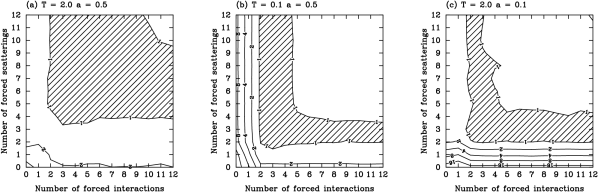
Figure 3: Contour plots of the relative errors in three trials of the slab geometry as functions of the number of forced scatterings and forced interactions. Trial (a) has $T=2$ and $a=0.5$, trial (b) has $T=0.1$ and $a=0.5$, and trial (c) has $T=2.0$ and $a=0.1$; in all cases $g=0.5$ and $\theta=45^{\circ}$. Contours are spaced by factors of 2. The hatched regions have the lowest errors.

To illustrate the importance of forced scatterings (§0.4.3) and forced interactions (§0.4.3), we have examined the relative errors in the emergent intensity in simulations of the slab geometry (§0.6) as functions of the number of forced scatterings and the number of forced interactions. In order to make the comparison fair, we ran each calculation for the same amount of processor time. The relative errors were estimated by partitioning the sample of pseudo-photons into 48 sub-samples.

We ran three trials with different values of $T$ and $a$. Trial (a) has $T=2.0$ and $a=0.5$, the same as the test case considered in §0.6, and is moderately optically-thick, with singly-scattered and doubly-scattered light dominating more-than-doubly-scattered light. Trial (b) has $T=0.1$ and $a=0.5$, and is optically-thin, with singly-scattered light dominating multiply-scattered light. Trial (c) has $T=2.0$ and $a=0.1$, and is moderately optically-thick, but has a low albedo, so singly-scattered light also dominates multiply-scattered light. In all cases we kept $\theta=45^{\circ}$ and $g=0.5$.

Figure 3 shows contour plots of the relative errors for these trials. The best results for trial (a), with $T=2$ and $a=0.5$, are obtained in a broad region with at least 4 forced scatters and 3 forced interactions. The best results for trial (b), with $T=0.1$ and $a=0.5$, were obtained for at least 2 forced interactions and at least 2 forced scatters. The best results for trial (c), with $T=2.0$ and $a=0.1$, were obtained for at least 2 forced interactions and at least 3 forced scatters. In all cases, however, the optimal region is roughly L-shaped. That is, excessive numbers of either forced scatters or forced interactions have little effect, but excessive numbers of both start to increase the error again.

The best errors for trials (a), (b), and (c) are roughly 7, 90, and 30 times smaller than for a naive implementation with no forced scatters or forced interactions Since the relative error in Monte Carlo calculations decreases as the square root of the computational effort, these optimizations represent savings in time of factors of roughly 50, 8000, and 1000.

These results can be understood qualitatively as follows. On average, the effect of forcing scatterings and interactions is to keep the pseudo-photon in the system for longer, which has two effects: (i) the pseudo-photon is more likely to contribute to derived quantities that depend on scattered light, which reduces the variance in these quantities, and (ii) the computational cost per pseudo-photons increases, so fewer can be followed, which increases the variance in derived quantities. In the cases examined here, the former is more important to begin with; for moderate numbers of forced scatterings and interactions, making each pseudo-photon more useful compensates for the smaller total number of pseudo-photons, and the variance is reduced. This is especially important if the system is optically thin (trial b) or if the albedo is low (trial c), as pseudo-photons can easily leave the system or be absorbed, and thereby make relatively little contribution to derived quantities.

However, if the number of both forced scatterings and interactions is excessive, each pseudo-photon is forced to remain in the system for many scatterings. This may reduced the variance of quantities derived from very highly scattered light, but it reduces the total number of pseudo-photons that can be considered, and thereby increases the variance of derived quantities that are dominated by moderately scattered light. Furthermore, the optimal region is L-shaped because, for the optical depths and albedos considered here, both excessive numbers of forced scatterings and excessive numbers of forced interactions are required to keep each pseudo-photons in the system for many scatterings; if one or the other is not excessive, the pseudo-photon is absorbed or escapes.

It is impossible to give a universally applicable rule to select a priori the optimal number of forced scatterings and interactions, as these quantities depend on the geometry and also on the particular quantity being calculated. However, the discussion in the previous paragraph implies that the optimal values for both will probably be roughly equal. Our experience suggests that two to four forced scatterings and interactions might be a useful rule of thumb; this number is not too far from optimal for any of the cases we have investigated.

Naive Monte Carlo algorithms are often considered ill-suited to optically-thin problems, as the overwhelming majority of photons escape without interacting. However, is not the case for more sophisticated algorithms that force the first few interactions, as our optically-thin trial demonstrates. A specialized single-scattering plus attenuation calculation would probably calculate the emergent singly-scattered intensity more efficiently, but a Monte Carlo calculation may well be more flexible and can directly account for multiply-scattered light.

0.8 Time-Dependence and Polarization

The algorithm as presented covers the time-independent transfer of unpolarized light. Both of these restrictions can be lifted quite easily.

The simplest way of including general time-dependence is to sample the range of times of emission, keep track of the travel time of the pseudo-photon within the system, and account for the travel time when computing quantities of interest. If only the source varies, it is probably more efficient to construct a “response function” for each quantity of interest which can be convolved with changes in the brightness of the source to predict the time-variation of that quantity.

Perhaps the simplest way to include polarization is to generalize the scalar statistical weight $w$ to a vector statistical weight $\mathbf{w}\equiv(w_{I},w_{Q},w_{U},w_{V})$, whose components correspond to the four components of the Stokes vector. The components will in general not be conserved upon scattering, but will transform according to the adopted scattering matrix. See, for example, Hillier (1991) and Whitney (1991).

0.9 Summary

We have presented and discussed a Monte Carlo algorithm for a restricted class of scattering problems. Our main contributions have been to formalize this algorithm, to present two test cases, and to investigate its efficiency. Important features of the algorithm are forced escapes, forced scatterings, and forced interactions. Using forced escapes to estimate the emergent intensity can be orders of magnitude more efficient than naively binning escaping pseudo-photons. Also, using a small number (two to four) of forced scatterings and forced interactions can significantly improve the efficiency of the algorithm for many problems, overwhelmingly so for optically-thin problems or those where the albedo is small.