On the Distribution of Orbital Poles of Milky Way Satellites
Abstract
In numerous studies of the outer Galactic halo some evidence for accretion has been found. If the outer halo did form in part or wholly through merger events, we might expect to find coherent streams of stars and globular clusters following similar orbits as their parent objects, which are assumed to be present or former Milky Way dwarf satellite galaxies. We present a study of this phenomenon by assessing the likelihood of potential descendant “dynamical families” in the outer halo. We conduct two analyses: one that involves a statistical analysis of the spatial distribution of all known Galactic dwarf satellite galaxies (DSGs) and globular clusters, and a second, more specific analysis of those globular clusters and DSGs for which full phase space dynamical data exist. In both cases our methodology is appropriate only to members of descendant dynamical families that retain nearly aligned orbital poles today. Since the Sagittarius dwarf (Sgr) is considered a paradigm for the type of merger/tidal interaction event for which we are searching, we also undertake a case study of the Sgr system and identify several globular clusters that may be members of its extended dynamical family.
In our first analysis, the distribution of possible orbital poles for the entire sample of outer ( kpc) halo globular clusters is tested for statistically significant associations among globular clusters and DSGs. Our methodology for identifying possible associations is similar to that used by Lynden-Bell & Lynden-Bell (1995) but we put the associations on a more statistical foundation. Moreover, we study the degree of possible dynamical clustering among various interesting ensembles of globular clusters and satellite galaxies. Among the ensembles studied, we find the globular cluster subpopulation with the highest statistical likelihood of association with one or more of the Galactic DSGs to be the distant, outer halo ( kpc), second parameter globular clusters. The results of our orbital pole analysis are supported by the Great Circle Cell Count methodology of Johnston et al. (1996). The space motions of the clusters Pal 4, NGC 6229, NGC 7006, and Pyxis are predicted to be among those most likely to show the clusters to be following stream orbits, since these clusters are responsible for the majority of the statistical significance of the association between outer halo, second parameter globular clusters and the Milky Way DSGs.
In our second analysis, we study the orbits of the 41 globular clusters and 6 Milky-Way bound DSGs having measured proper motions to look for objects with both coplanar orbits and similar angular momenta. Unfortunately, the majority of globular clusters with measured proper motions are inner halo clusters that are less likely to retain memory of their original orbit. Although four potential globular cluster/DSG associations are found, we believe three of these associations involving inner halo clusters to be coincidental. While the present sample of objects with complete dynamical data is small and does not include many of the globular clusters that are more likely to have been captured by the Milky Way, the methodology we adopt will become increasingly powerful as more proper motions are measured for distant Galactic satellites and globular clusters, and especially as results from the Space Interferometry Mission (SIM) become available.
1 Introduction
Models for structure formation in the universe that include a dominant cold dark matter (CDM) component predict a hierarchical formation process where large structures are formed by the merging of smaller CDM halos. Numerical simulations (e.g., Moore et al., 1999; Klypin et al., 1999) seem to indicate that galaxies form in a similar fashion as do galaxy clusters, as subgalactic CDM halos merge to form galaxy sized halos. These simulations support the idea that the Milky Way formed as an aggregation of smaller units, however, there is some controversy because the simuluations overpredict the number of subgalactic halos that remain at in a Local Group type environment. In the Local Group, there are two populations of subGalactic objects that may be related to the CDM halos in numerical simulations: globular clusters and dwarf galaxies. It is possible that there remains information on the growth of structure in the Milky Way system encoded in the current globular cluster and dwarf satellite galaxy (hereafter, DSG) populations found in orbit around the Milky Way.
Globular clusters are often used as archetypal objects, and their current properties can not only be used to constrain their formation and evolutionary histories, but those of the Galactic stellar populations they trace. In the Milky Way, the population of globular clusters has traditionally been split into an inner and an outer population, separable by metallicity (Zinn, 1980). More recently, it has been shown that these “halo” (outer) and “disk” (inner) populations can be further subdivided when additional properties are considered in addition to metallicity.
The properties of the outer ( kpc) globular clusters of the Milky Way suggest that they are, and trace, a distinct population with formation and evolutionary histories different from those of the more tightly bound, inner ( kpc) globular clusters. The outer globular clusters share similar kinematical, metallicity, age, and spatial distributions as halo stars (e.g., Zinn, 1985, 1996) and are thus usually assumed to be representative of the halo stellar population. It is more difficult to assign individual inner globular clusters to specific stellar populations, because of the overlap in properties between the bulge, thin disk, thick disk, and halo populations near the center of our Galaxy; however, for the most part the inner globular clusters tend to have kinematical, metallicity, and spatial distributions closer to those of the bulge or disk than of the halo (e.g., Zinn, 1985; Armandroff & Zinn, 1988; Minniti, 1995; Zinn, 1996), although Burkert & Smith (1997) use dynamical arguments to assign some of the highest metallicity, inner globular clusters to an inner halo population, distinct from a “bar” population and a 5 kpc ring population. The kinematical and spatial differences found between the inner and outer globular cluster subpopulations (specifically the existence of retrograde orbiting globular clusters found among the latter group) support the Galactic formation scenarios of Searle (1977) and Searle & Zinn (1978), who proposed that the outer halo of the Milky Way may have formed through the infall and accretion of gas and stars from “fragments” after the collapse of the proto-Galactic cloud that produced the inner Milky Way. The accretion into the halo of globular clusters that formed in fragments can account for the observed apparent age spread in globular clusters that may be as large as 5 Gyr by some accounts (for a recent review see Sarajedini et al., 1997). Although the magnitude of the age spread among globular clusters is still uncertain (e.g., Stetson et al., 1996; VandenBerg, 1997) any significant halo age spread ( Gyr) is incompatible with the timescale for a single collapse for halo formation as originally proposed in the Eggen, Lynden-Bell, & Sandage (1962) model.
Studies by Kunkel & Demers (1976) and Lynden-Bell (1982) found spatial alignments among the DSGs, fueling speculation that these objects may be the fragments proposed in the Searle & Zinn (1978) accretion model of the Galactic halo. Kunkel & Demers (1976) postulated that a group of six DSGs and four red horizontal branch globular clusters, which they denoted the “Magellanic Plane Group”, are relics of a past tidal interaction between the Magellanic Clouds and the Galaxy since the DSGs, clusters, and the Magellanic Clouds lie near a great circle that is nearly coincident with the Magellanic (HI gas) Stream. Subsequently, Kunkel (1979), using contemporary radial velocity data, presented evidence for motion along a single orbit by the Magellanic Plane DSGs and globular clusters, which provided further support for the tidal disruption hypothesis. Lynden-Bell (1982), adopting a different orbital indicator, suggested that one could identify objects on similar orbits (i.e. remnants of a single merger event) by looking at their angular momentum axes, assumed to be given by where is the Galactocentric radius vector of an object and is the position angle of the tidal extension of the object. For example, he noted a coincidence between the tidal elongation of the Ursa Minor dwarf galaxy and the orientation of the Magellanic Stream. Looking at the spatial distribution of all known Milky Way DSGs and their tidal elongations, Lynden-Bell identified two “streams” of objects, a Magellanic stream333Hereafter, when we refer to the “Magellanic stream”, we mean the great circle defined by Lynden-Bell (1982) that contains the LMC, SMC, Ursa Minor, and Draco DSGs. This is to be contrasted to the “Magellanic Stream”, the large complex of HI gas associated with the Magellanic Clouds., and an “FLS” stream that contains the Fornax, Leo I, Leo II, and Sculptor dwarf galaxies. According to Lynden-Bell (1982), these spatial alignments may have arisen from the tidal disruption of a Greater Magellanic Galaxy and a Greater Fornax Galaxy. Given recent evidence for the disruption of DSGs themselves (e.g., Carina and Ursa Minor; Majewski et al., 2000; Palma et al., 2001), it is possible that these dwarf galaxies represent an intermediate phase in the total accretion of larger, LMC-like satellites by the Milky Way.
Both Kunkel & Demers (1976) and Lynden-Bell (1982) included specific globular clusters, generally those in the outer halo, in their alignment schemes. Interestingly, it is these same clusters that played a significant role in shaping the original Searle & Zinn (1978) picture and which have continued to spark interest in the possibility that the Milky Way halo continues to assimilate debris from the disruption of chemically distinct systems. In an influential recent study, Zinn (1993a) found evidence for significant kinematical differences between two populations of halo globular clusters discriminated by a combination of the Lee et al. (1994) index of horizontal branch morphology and [Fe/H]. In this new scheme, Zinn (1993a) refers to the two subdivisions of outer halo globular clusters as the “Old Halo” and “Young Halo” globular clusters under the assumption that the second parameter of horizontal branch morphology is age. The “Young Halo” globulars are found to have a mean rotational velocity that is retrograde and with a large line-of-sight velocity dispersion of km/sec. This is in contrast to the “Old Halo” globular clusters, which have a mean prograde rotational velocity and a much smaller . Zinn (1993a) suggests that the observed flattening in the spatial distribution of the combined Old Halo and Disk globular populations, as well as the correlation of [Fe/H] to Galactocentric radius () within those combined populations, imply that the Old Halo globulars and the Disk globular clusters together may be products of the same formation mechanism, perhaps an ELS-like collapse. On the other hand, the spherical spatial distribution, lack of a metallicity trend with , and the possible retrograde rotation of the Young Halo globular clusters implies that they may have formed separately than the DiskOld Halo globular clusters, and then were later accreted by the Milky Way á la Searle & Zinn (1978). In a more recent study, Zinn (1996) subdivides the halo globular clusters further, into three populations, and adopts terminology that is less specific regarding the possible origin of the second parameter effect. The “RHB” (red horizontal branch) group is essentially the same as the Young Halo group from Zinn (1993a). However, the Old Halo group he now splits into a “MP” (metal-poor) group with Fe/H and a “BHB” (blue horizontal branch) group with Fe/H (the metallicity range where the second parameter effect operates). We adopt the more recent terminology of RHB vs. BHB/MP since it makes no assumption as to the origin of the second parameter effect.
It is now recognized that many of the most distant outer globular clusters are predominantly of the RHB type, and Majewski (1994) shows that the outer halo globular cluster/DSG connection may pertain to the origin of the second parameter effect. Like Kunkel & Demers (1976), who included several red horizontal branch clusters as part of their Magellanic Plane group, Majewski (1994) found a spatial alignment between a sample of Young Halo globular clusters and the FLS stream galaxies. Majewski found that if one fits an orbital plane to the positions of the FLS stream DSGs similar to Lynden-Bell’s (1982) orbital plane for the FLS stream, the positions of the most distant outer halo, red horizontal branch (young) globular clusters (as well as the more recently discovered Sextans dwarf and the Phoenix dwarf) are found to be correlated with the best-fit plane. Fusi Pecci et al. (1995) also fit a plane to the spatial distribution of the Galactic DSGs, and found that many of the globular clusters considered to be younger than the majority of Galactic globular clusters (which are all RHB type) lie on their best fit plane.
The most striking evidence for a tidal capture origin for some outer halo globular clusters comes from the recently discovered (Ibata et al. 1994, 1995) Sagittarius dwarf spheroidal (Sgr). This DSG is currently 16 kpc from the Galactic center, closer than any of the other Milky Way DSGs. A consequence of its apparently small perigalacticon is that the Sagittarius dwarf shows evidence for ongoing tidal disruption by the Milky Way (Ibata et al., 1995; Mateo et al., 1998; Johnston et al., 1999). Of particular interest to our discussion here are four globular clusters (M54, Arp 2, Ter 7, and Ter 8) with Galactocentric positions and radial velocities very similar to those of Sagittarius. It appears that at least some of these four globular clusters originally belonged to Sagittarius and are in the process of being stripped from their host by the Milky Way. Recently, Dinescu et al. (2000) have determined the proper motion of Pal 12 and argue that it too may have originally belonged to the Sgr.
Lynden-Bell & Lynden-Bell (1995, hereafter LB295) recently pioneered a technique for identifying other potential cluster/DSG associations using the positions and radial velocities of the entire sample of globular clusters and DSGs. They identify candidate streams similar to the Magellanic stream and FLS stream by selecting families of objects whose “polar paths” (great circles identifying all possible locations of their orbital poles, see §3.1 and §5 below) share a nearly common intersection point and that also have similar orbital energies and angular momenta as derived using current radial velocities and an assumed Milky Way potential. We revisit the technique of LB295 in our attempt to address the following questions:
-
•
Can we improve the case for association of globular clusters with DSGs? Can we develop a more statistical foundation for this suggestion?
-
•
Can we point to specific dynamical families in the halo to make previously proposed associations of DSGs and/or globular clusters less anecdotal?
-
•
Can we provide specific targets for follow-up study to test the “dynamical family” hypothesis?
-
•
Can we verify the suggestion that it is the RHB globular clusters that are more associated with the tidal disruption process?
-
•
What are the limitations in this type of analysis?
Previous, related investigations have all relied solely on positional alignments (and in some cases radial velocities), or have estimated orbital properties relying on assumptions about the shape of the Galactic potential and the objects’ transverse velocities. In this work, we first reinvestigate positional globular cluster and DSG alignments by applying statistical tests to the results of an LB295 type “polar path” analysis. We then search for possible dynamical groups among the (still relatively small sample of) Galactic globular clusters and DSGs having available radial velocity and proper motion measurements.
2 The Sample of Halo Objects
Positions and radial velocities of all globular clusters were adopted from the 22 June 1999 World Wide Web version of the compilation by Harris (1996). Satellite galaxy positions were taken from the NASA/IPAC Extragalactic Database (NED444The NASA/IPAC Extragalactic Database (NED) is operated by the Jet Propulsion Laboratory, California Institute of Technology, under contract with the National Aeronautics and Space Administration.), radial velocity data from the recent review by Mateo (1998) and proper motions (for all objects) from various sources, which are listed in Table 1. In cases where multiple proper motions have been published for globular clusters and DSGs, we have selected the measurement with the smallest random errors. The proper motion that was adopted for analysis is listed first in Table 1 for objects with multiple measurements. However, for most globular clusters with multiple independent proper motion measurements, the position of the orbital pole is fairly insensitive to the differences between measurements. Exceptions are discussed in §6.1.
For the DSGs and globular clusters in our analysis, we used the adopted position, distance, radial velocity, and proper motion to determine Galactic space velocities, , and their one sigma errors using the formulae from Johnson & Soderblom (1987). These velocities were transformed to the Galactic standard of rest using the basic solar motion (Mihalas & Binney, 1981) of km/sec (the difference between this value and any of the more recent determinations is significantly below the proper motion velocity errors) and a rotational velocity of the Local Standard of Rest (LSR) of km/sec (Kerr & Lynden-Bell, 1986). The Galactocentric Cartesian radius vectors, , for the DSGs and clusters were calculated using an adopted value of 8.5 kpc (Kerr & Lynden-Bell, 1986) for the solar Galactocentric radius. In instances where orbital parameters were calculated for our sample objects, the Galactic potential was assumed to be that of Johnston et al. (1995)
While proper motion errors tend to be large (sometimes of order 100%) for most objects, the radial velocity errors are often very small compared to the magnitude of the radial velocity itself. The propagated errors in the velocities depend strongly on the ratio of the magnitude of the radial velocity to the magnitude of the tangential velocity, after one transforms to the Galactic Cartesian system. For example, Ursa Minor has a radial velocity of km/sec, while its proper motion translates to a transverse velocity of magnitude km/sec. Even though its proper motion error is large, since its radial velocity makes up the majority of its total space velocity, the error in its total velocity is only %. This “reducing” effect in the total error is reflected in the length of the Arc Segment Pole Families (see §3) for some of those objects with large proper motions errors (e.g., Ursa Minor).
The final sample used in §5 includes the 147 Milky Way globular clusters from the Harris (1996) compilation and the LMC, SMC, Draco, Ursa Minor, Sculptor, Sagittarius, Fornax, Leo I, Leo II, Sextans, and Carina of the Milky Way DSGs. We also included the Phoenix dwarf galaxy, however, this object was left out of some of our analyses due to its uncertain connection with the Milky Way. From this sample of 147 globular clusters and 12 galaxies, we collected proper motion data from the literature for 41 clusters and 6 galaxies (Table 1), which we use for the orbital pole analysis in §6.
3 The Orbital Pole Family Technique
If we assume that the outer halo of the Milky Way was formed at least partially through the tidal disruption of dwarf galaxy-sized objects, we may expect to observe the daughter products of these mergers. As described in the Introduction, there are spatial alignments of DSGs and young globular clusters that suggest they may be sibling remnants of past accretion events. We wish to improve upon previous searches for spatial alignments by identifying groups of these objects that share a nearly common angular momentum vector. The LB295 technique relies fundamentally on positional data for these clusters. These data are not going to change in any significant way, and the only way to improve on this basic technique is through more complete, statistical analyses of the sample. We do this here. However, by taking advantage of proper motion data, an improved, modified LB295 technique can be applied, and this new approach will always increase in usefulness as more and better proper motion data become available. Thus, our search technique has roots in the methodology of LB295, but we take two steps forward from their analysis: (1) We take advantage of a simple two-point angular correlation function analysis to address possible alignments in a stellar populations context, and (2) we take advantage of the growing database of orbital data for outer halo objects to search for associations among refined locations for the LB295 “polar paths”.
3.1 Constructing an Orbital Pole Family
As discussed by LB295, from knowledge of only its vector one can construct a family of possible orbital poles for each Galactic satellite. The basic assumption underlying pole family construction is that each satellite orbits in a plane containing the object’s current position and the Galactic center. The family of possible orbital poles is simply the set of all possible normals to the Galactocentric radius vector for a particular satellite (Figure 1). Clearly it is desirable to limit further the family of possible orbital poles if at all possible. There are two limiting cases: If one has no information save the object’s Galactic coordinates, the family of possible normals traces out a great circle on the sky. This is the basis of the LB295 method: Any set of objects constituting a dynamical family (i.e., a group of objects from a common origin and maintaining a common orbit), no matter how spread out on the sky, will have “Great Circle Pole Families” (GCPFs) that intersect at the same pair of antipodal points on the celestial sphere. Thus, searching for possible dynamical families, orbiting in common debris streams, means plumbing the set of all GCPFs for common intersection points. As a further constraint, LB295 derived “radial energies” (an approximation to the orbital energy that are derived using measured heliocentric radial velocities) to eliminate objects from streams with grossly different orbital parameters.
The other limiting case occurs if one knows the space velocity for the object with infinite precision. Then, the pole family consists of one point, the orbit’s true pole. In reality, however, space motions of Galactic satellites have fairly large uncertainties, generally, in large part due to the proper motion errors. Thus, we never truly achieve a well-defined orbital pole point. However, even with rough space motions we can constrain the true pole to lie along an arc segment (an “Arc Segment Pole Family”, or ASPF) rather than a great circle (Figure 1). The better the space motion errors, the smaller the arc segment, which, in the limit of no error, is a point. LB295 provided lists of potential streams derived with their GCPFradial energy technique with the understanding that in the end, proper motions must be measured to confirm stream membership. Although proper motions remain unavailable for the majority of the objects found in the streams of LB295, we can search the sample of globular clusters and DSGs with proper motions for associations of their ASPFs, which produces better defined streams than those selected with the GCPF method.
3.2 Physical Limitations of the GCPF Technique
Although techniques exist (e.g., the Great Circle Cell Counts technique of Johnston et al., 1996) to search for the stellar component of tidal debris among large samples of Galactic stars, orbital pole families can be a powerful tool in the search for remnants of past merger events among even small samples of objects in dynamical associations spread out over the celestial sphere. In a spherical potential, the daughter products of a tidal disruption event should have nearly identical orbital poles, indicative of a common direction of angular momentum. In such an ideal case, the GCPFs of the daughter objects will all intersect at a pair of antipodal points on the sky (another way of denoting that the objects all lie in one plane).
In practice, however, we do not expect to find perfect coincidences among the orbital poles of tidal remnant objects for a number of reasons:
-
1.
Even in a spherical potential the debris orbits will be spread in energy about the disintegrating satellite’s orbital energy, with a typical scale (see e.g., Johnston, 1998, for a discussion)
(1) where is the tidal radius of the satellite (see King, 1962), is the parent Galaxy potential, is the circular velocity of the Galactic halo, is the satellite’s mass, is the mass of the parent galaxy enclosed within the satellite’s orbit, and the last equality defines the tidal scale . This spread in energy translates to a characteristic angular width to the debris.
-
2.
If the parent Galaxy potential is not perfectly spherical, then the satellite’s orbit does not remain confined to a single plane. For example, differential precession of the orbital pole of debris from a satellite may be induced, so remnant objects with slightly different orbital energies and angular momenta that are found at different phases along the parent satellite’s orbit will have different orbital poles. Moreover, Helmi & White (1999) point out that debris from inner halo objects is not expected to retain planar coherence. Indeed, some objects currently found within kpc show chaotically changing orbital planes (e.g., the cluster NGC 1851; see Dinescu et al., 1999b). Because the GCPF/ASPF technique depends on the orbital poles of debris remaining approximately constant, differential precession and other dynamical effects act to degrade the signal we seek. As shown in Figure 2, however, outside of kpc, orbital pole drifting is a small effect, and not likely to affect orbital pole alignments greatly. Thus, the GCPF/ASPF technique should be robust when probing the alignments of outer halo objects, however for inner halo objects it will only be useful for relatively recent disruptions.
- 3.
-
4.
If the Galaxy’s potential evolves significantly (e.g., through accretion of objects or growing of the disk) this could cause initially aligned orbital poles of objects to drift apart (see LB295 and Zhao et al. 1999 for a more complete discussion).
However, if the timescales for orbital pole drifting in the outer halo are long enough, the true poles of tidal remnants should remain relatively well aligned, and the GCPFs of these remnants may all intersect within a small region on the sky (where “small” can be estimated on the basis of the tidal scale, for example). Indeed, the argument may be turned around; given the various processes that tend to cause drift among orbital poles, any well-defined, multiple GCPF crossing point region that remains today is of particular interest. For example, the GCPFs of the Magellanic stream DSGs (LMC, SMC, Draco, and Ursa Minor) are nearly coincident, due to the spatial alignment of these objects on the sky, and their GCPFs share nearly common intersection points (dashed lines in Figure 3). This nexus points to the oft-cited possibility of a dynamical connection for these four objects.
However, while the GCPFs’ nearly common crossing points indicate a possible association, the true orbital poles of these objects can lie anywhere on their respective Great Circle Pole Families and do not necessarily need to lie near the crossing point. Thus, nearly common crossing point of the GCPFs of several DSGs does not indicate with any certainty that the objects involved are truly the remnants of a past tidal disruption, since the GCPFs contain no information about the orbital energy or the magnitude and direction of the angular momentum for each object. Therefore, one may use common crossing points to identify objects that are potentially dynamically linked, but then other information, such as the orbital energy and momentum, must be used eventually to check the likelihood of the dynamical associations. For example, in LB295, measurements of the radial velocity of each satellite and an assumed model of the Galactic potential were used to estimate the orbital energies and specific angular momenta of their proposed candidate dynamical family members. LB295 also assumed that the tidal elongations of the DSGs lie along their orbital paths, which allowed them to hypothesize a true pole location for each.555In the particular case of the Magellanic stream family, this assumption is supported, for example, by the observation of Oh, Lin, & Aarseth (1995) that the flattenings observed by Irwin & Hatzidimitriou (1993, 1995) in the outer parts of Draco, Carina, and Ursa Minor appear to align with the plane defined by the Magellanic Stream.
Clearly, approximate knowledge of the true space motions of Milky Way satellites is an improvement over the basic LB295 GCPF technique, since one may constrain the true orbital pole to lie somewhere along an ASPF. Moreover, one can estimate the orbital energy (within an assumed potential) and angular momentum directly, rather than relying on assumed orbits. For example, in Figure 3, we show the ASPFs (thick lines) for the Milky Way DSGs, where the ASPFs are constructed using the space motion data available in the literature (see also Majewski, Phelps, & Rich, 1996). For reference the poles of all previously proposed DSG/globular cluster alignment planes, including Lynden-Bell’s (1982) Magellanic stream (MS), Kunkel’s (1979) Magellanic Plane Group (MPG), and the MP-1 and MP-2 planes of Fusi Pecci et al. (1995), are included. The Fornax-Leo-Sculptor plane of Lynden-Bell (1982) is illustrated with the “FSS” (LB295) point and the “FLLSS” point (Majewski 1994). The Andromeda plane (AND) of Fusi Pecci et al. (1995) is also included for reference. The space velocity data, represented by the ASPFs in Figure 3, support the notion of a true “dynamical group” among the Magellanic stream DSGs since their ASPFs do not appear to be randomly distributed around the sky, but tend to lie remarkably near the multiple GCPF crossing point region, which lies near the poles of the MS, MP-2, and MPG alignment planes. In addition, Figure 3 illustrates that among DSGs with measured proper motions, all are on nearly polar orbits (i.e. their orbital poles are near the Galactic equator). Since polar orbits are the least affected by precession, we expect that the ASPFs for these objects have remained nearly constant over the lifetime of each DSG.
Although knowledge of the space velocities of Galactic satellites allows one to select objects with similar orbital dynamics with some confidence, the current measurements of space velocities for most satellites are not of the quality necessary to perform this task with definitive results. Since this limitation in data quality does not yet allow the precise identification of dyamical families among the Galactic satellite population, other information must presently be used to reinforce the inclusion of (or to eliminate from consideration) potential stream members identified by orbital pole alignments. LB295 solved this dilemma by inverting the problem; objects were selected with velocities and distances that produced radial energies consistent with stream membership, and only then were the potential orbital pole families of these objects searched for possible alignment.
The goal of this work is similar to that of LB295, however, we differ in not relying on the radial energy technique to discriminate dynamically associated satellites from chance alignments, since this was thoroughly pursued in that paper. Rather, we concentrate on the more general view of what can be learned with full phase-space information – both with the current data and with an eye toward refinements in the distances and space velocities of Galactic satellites and clusters to be delivered by the astrometric satellite missions SIM, GAIA, FAME, and DIVA. Therefore, our philosophy is to pursue a more liberal listing of possible associations based on orbital polar alignments that can be tested with these future data.
4 Case Study of the Sgr System
Because Sagittarius is a paradigm for the type of tidally disrupted system for which we are searching, it is worthwile to explore this example in detail. Others have proposed that Sgr is currently losing its globular clusters to the Milky Way; for example, Da Costa & Armandroff (1995) argued that Terzan 7, Terzan 8, and Arp 2 all belonged to Sgr and may be in the process of being tidally removed from the galaxy (see also Ibata et al., 1995), while Dinescu et al. (2000) proposed that Pal 12 was removed from Sgr during a previous pericentric passage. Since stellar debris from Sgr has been identified at increasingly displaced positions on the sky (Mateo et al., 1998; Majewski et al., 1999a; Ivezić et al., 2000; Ibata et al., 2001a) we investigate here the possibility that there may be other captured Sgr clusters distributed among the Galactic globular cluster population.
In Figure 4, we show the Sgr ASPF along with the GCPFs for a sample of globular clusters selected as potential Sgr debris based on the proximity of their GCPFs to the Sgr ASPF. The globular clusters in the sample, M53, NGC 5053, Pal 5, M5, NGC 6356, M54, Terzan 7, Terzan 8, and Arp 2 were chosen to satisfy two criteria: (1) their GCPFs come within of the Sgr ASPF (see §3.2 for a discussion of the expected angular width of tidal debris derived from , where was assumed to be ), and (2) kpc. Of this group, NGC 6356 () has properties similar to the Burkert & Smith (1997) metal-enriched, inner halo population, which they argue formed during the collapse phase in the Galaxy’s formation. However, an alternative explanation for NGC 6356’s halo-like orbit could be accretion from a Galactic DSG; we note that its metallicity is similar to that of the Sgr cluster Terzan 7. On the other hand, M53 and NGC 5053 are more metal poor than the previously identified Sgr clusters ( and , respectively). Of the remaining candidate Sgr clusters, four are those previously proposed to be Sgr clusters (M54, Ter 7, Ter 8, and Arp 2); the other two are Pal 5 and M5, which are both second parameter, red horizontal branch clusters. The physical and orbital parameters (orbital energy, orbital angular momentum, , , , , , and concentration parameter) are tabulated in Table 2 for the known Sgr globular clusters (bottom of table) and for the new candidate Sgr clusters presented here (top of table).
The ASPFs of the three clusters in Figure 4 with measured proper motions (M53, Pal 5, and M5) are plotted as thick, solid lines. Pal 5 is shown with two ASPFs, since the Cudworth et al. (2001) and Scholz et al. (1998) proper motions are so discrepant that the resultant ASPFs lie almost apart. It is interesting to note that like Sgr, M53, Pal 5, and M5 are apparently on nearly polar orbits. Perhaps these clusters were Sgr clusters, but precession has caused their poles to drift from that of Sgr? These three clusters are at kpc, where precession effects are more significant (Figure 2 shows drifts of up to 50∘ at 16 kpc), however nearly polar orbits generally precess more slowly than orbits with smaller inclinations. The orbital parameters suggest that Pal 5 is on an orbit unlike that of Sgr. With either proper motion, the orbital energy and angular momentum of Pal 5 differ from Sgr, but there is enough uncertainty in the differences that an Sgr debris orbit can not be completely ruled out. However, the orbital energy and angular momentum of M53 are very similar to Sgr ( and kpc km/sec respectively and and km2/sec2 respectively). For M5 the values are more discrepant ( and ), however, the proper motion of M5 is of lower precision than either that of Pal 5 or M53.
The available data do not allow us to definitively identify any of these clusters as captured Sgr clusters, however several of the candidates are similar enough to the system of Sgr globular clusters to warrant further investigation. Dinescu et al. (2000) argue for Pal 12 as an Sgr cluster due to its dynamics, and also because its metallicity, mass, and concentration are similar to the other Sgr clusters. Pal 5 has a metallicity, mass, and concentration similar to Pal 12, Ter 7, Ter 8, and Arp 2, however its orbit seems too different from that of Sgr to be definitively considered a captured Sgr cluster. M53 is more metal poor, more massive, and more centrally concentrated than all the Sgr clusters except for M54, which is postulated to be the nucleus of Sgr, however M53’s dynamics seem to match well with Sgr. Finally, M5 has a metallicity similar to the Sgr clusters, dynamics that may be consistent with Sgr, yet it too is more massive and centrally concentrated than Pal 12, Ter 7, Ter 8, and Arp 2. This case study of Sagittarius demonstrates the potential of the pole analysis technique to uncover dynamical associations and presents several new candidates (Pal 5, M53, M5, and NGC 6356) for an extended Sgr dynamical family.
5 Great Circle Pole Family Analysis
Now, we search the entire sample of halo globular clusters and DSGs for nexuses of multiple GCPFs similar to that seen among the Magellanic stream DSGs (Figure 3). Although the core of the GCPF analysis presented here is not significantly different than that of LB295, our study differs in that we (1) investigate the possible dynamical association of various distinct subpopulations of globular clusters with Milky Way DSGs and (2) compare the probability of all potential dynamical associations in a statistical, rather than anecdotal, manner.
We analyze the GCPFs of a sample of objects in the following way:
-
1.
For each pair of objects in the sample, calculate the two points along their respective GCPFs where there is an intersection. We remind the reader that this introduces a redundancy due to symmetry around the antipodes, but this redundancy has been taken into account during the analysis.
-
2.
Calculate the angular distance (along the connecting great circle, i.e., the minimum angular distance) between each crossing point and every other crossing point.
-
3.
To assess the true statistical significance of clustering among the GCPF crossing points, we calculate the two point angular correlation function for the crossing points of various subsamples and compare to the results for other subsamples.
There are various ways to estimate , and we adopted the technique for calculating the estimator outlined in Landy & Szalay (1993). The estimator compares the distribution of angular separations of data/data (DD) pairs to that of random/random (RR) pairs (a discussion of the random data generation is included in Appendix A). One cannot use other estimators (such as the estimator; Landy & Szalay 1993) that rely on, for example, the comparison of DD pairs to a cross-correlation of the data points to random points (DR pairs) due to the nature of GCPF crossing points. The problem lies in the fact that there is an intrinsic correlation in crossing point data because all points on the celestial sphere are not equally likely to have a crossing point: Only those points that lie along two great circles may be crossing points. The same intrinsic correlation of crossing point location applies to any randomly generated set of GCPF crossing point data, as long as the crossing point distribution is derived after generating a random set of constraining great circles, rather than simply generating random crossing points that lie anywhere on the celestial sphere. For example, the orientations of the great circles in the real dataset are completely uncorrelated to the positions of the great circles in the random dataset, so DR cross-correlations do not have the intrinsic correlation found in the DD and RR data and false signal amplitudes will be generated in comparison of DD to DR pairs. In such a misapplication of the technique, then, since the positions of the great circles in the real data are independent of the positions in the randomized data, the DD/DR estimators would measure the amplitude of the clustering as well as the amplitude of the correlation in the positions of great circles in the real data, and therefore artificially inflate the amplitude of . On the other hand, the appropriate, DD/RR, estimators measure only the amplitude of the clustering in the data, since the same intrinsic correlation is contained in both the DD and RR pairs (if the great circles are randomized fairly; see Appendix A) and falls out when the ratio is taken.
The total sample of globular clusters and Milky Way DSGs is very large. Since there will be crossing points, the signature of a true dynamical grouping can be lost in the “noise” of random crossing points. Moreover, we suspect that there may be some correlation of physical characteristics in the debris from a common progenitor. Thus, variously selected samples of similar objects may show a higher degree of orbital coherence. For example, the Searle & Zinn (1978) fragment accretion hypothesis was motivated by the predominance of the second parameter effect in the outer halo globular clusters. We therefore can hope to improve the signal-to-noise in potential dynamical families with judicious parsing of the sample into physically interesting subsamples.
It has been argued that selecting globular clusters by metallicity (e.g., Rodgers & Paltoglou, 1984), by horizontal branch morphology (e.g., Zinn 1993, 1996), or by Oosterhoff class (van den Bergh, 1993) will separate the globular cluster population into distinct sub-populations with different kinematical properties that may in some cases be indicative of an accretion origin. We have attempted to reproduce some of these divisions to determine if one particular sub-population has a greater incidence of GCPF crossing point clumping than the others. The results are summarized in the following sections.
5.1 Zinn RHB vs. Zinn BHB/MP Globular Clusters
After dividing globular clusters into two types using the [Fe/H] vs. HB morphology parameter diagram (Lee et al., 1994), Zinn (1993a) found that kinematic differences exist between the “Old Halo” (BHB/MP) and “Younger Halo” (RHB) populations, evidence that supports the accretion model of the second parameter, RHB clusters, which predominate in the outer halo. Majewski (1994) has shown evidence for a spatial association between a sample of Zinn RHB globulars (specifically, those with the reddest HBs) and the Fornax–Leo–Sculptor stream of DSGs, which suggests that these may be related to a common Galactic tidal disruption event. We support these spatial and kinematical associations among the RHB globulars with the results of our GCPF technique. Using the metallicity and HB morphology data from the Harris (1996) compilation and adopting the same partitioning scheme as in the Zinn (1993a) paper, we separated all non-disk Milky Way globular clusters into the RHB and BHB/MP types. In so doing, we take into account the recommendations of Da Costa & Armandroff (1995) to include Ter 7, Pal 12, and Arp 2 in the RHB group. Since we are interested mainly in the outer halo, where dynamical families are expected to be best preserved from phase mixing (Helmi & White, 1999), and where there is minimal contamination by disk clusters, we also impose an kpc cutoff for both groups. The final samples, listed in Table 3, contain 22 BHB/MP globular clusters and 26 RHB globular clusters. We analyze both samples twice: either including or excluding the Milky Way DSGs.
From a comparison of the distribution of crossing points for the Zinn RHB globular clustersDSGs to the crossing points for the Zinn BHB/MP globular clustersDSGs (Figure 5), it is clear that there are several large groupings in the RHBDSG sample that are absent or are much smaller in the BHB/MPDSG sample. It is especially interesting to note that the largest grouping found in both datasets is located where the GCPFs of the FL2S2 DSGs cross those of the Magellanic stream Group DSGs, near (see Figure 3). However, when one looks at the crossing points of only the RHB or BHB/MP globular clusters without including the GCPFs of the DSGs, there is still a large grouping of crossing points in the RHB globular cluster data, but no crossing points in this region in the BHB/MP globular cluster data. This indicates that this particular excess of crossing points near in the BHB/MPDSG sample is entirely due to the DSGs, while in the RHBDSG sample there are a large number of globular cluster/globular cluster crossing points also found in the region. Moreover, there appears to be no clustering of GCPF crossing points in the BHB/MP globular cluster sample that is anywhere near the size or density of that seen in the RHB cluster sample.
The two point angular correlation function calculation shows that the RHBDSG sample has a larger amplitude than that of the BHB/MPDSG sample out to scales of (Figure 6, upper panel). The amplitude for the BHB/MPDSG sample is actually consistent with it being a random distribution (i.e. DD/RR). This is statistical verification of what one sees by eye: The crossing points for the RHB globular clusters DSGs are more clumped than those of the BHB/MP globular clustersDSGs. If one looks at the amplitude for the globular cluster samples alone (Figure 6, lower panel), the sample size is sufficiently small that there is a large overlap in the error bars for points , so it is difficult to prove definitively that the RHB globular clusters taken alone are more clumped than the BHB/MP globular clusters. However, there does appear to be a larger amplitude for the RHB globular clusters than for the BHB/MP clusters, particularly for .
The majority of the clustering signal comes from the large clump of crossing points near . This group of crossing points near the equator supports the notion that polar orbits are preferred not only by the DSGs (a notion that is verified by the actual orbital data we have for some of the DSGs), but perhaps by the second parameter clusters (which we find potentially to be associated with these DSGs) as well. Applying the cluster finding algorithm described in §6.2 to the distribution of crossing points, we find that the GCPFs of the following globular clusters create the excess of crossing points near the equator: Pyxis, IC 4499, Pal 3, Pal 4, M3, M68, M72, M75, NGC 4147, NGC 6229, and NGC 7006. If we apply a less conservative angular cutoff when we determine which crossing points contribute to this excess, we find that Pal 12, AM1, NGC 2808, Rup 106, and NGC 6934 also contribute to the size of the clump of crossing points. Figure 7 shows a plot of the pole families for the 11 globular clusters selected with the conservative partition; a discussion of the ASPF distribution of the four globular clusters in this group with measured proper motions is in §6.3. Although the DSGs have been previously separated into two groups, the Magellanic stream group and the FL2S2 group, we must note here that the GCPFs of the Magellanic stream galaxies intersect those of the FL2S2 galaxies in the region near . Thus, the large clump of crossing points (which appears to be made of two subclumps; one due to the Magellanic stream group galaxies and one due to the FL2S2 galaxies) contains crossing points derived from the GCPFs of all of the globular clusters listed above and both Magellanic stream and FL2S2 galaxies. Therefore it is possible that many of these globular clusters belong to either the Magellanic stream or the FL2S2 groups. Of this group of 11 globular clusters, Pal 3, Pal 4, and M75 are part of the group of proposed FL2S2 globular clusters of Majewski (1994), IC 4499 is part of the MP-1 plane of Fusi Pecci et al. (1995), and Kunkel & Demers (1976) include Pal 4 and NGC 7006 in their Magellanic Plane group.
Frenk & White (1980) found that the radial velocities of 66 globular clusters with kpc are consistent with a systemic rotation around the Galactic pole of 6026 km/sec. More recently, Zinn (1985, 1993) used the Frenk & White (1980) technique to show that the globular clusters with [Fe/H] have disklike rotation velocities, while the more metal-poor globular clusters have a marginally significant net rotation with a large velocity dispersion. In all of these studies, the globular clusters were assumed to have a systemic rotation around the same axis as the Milky Way’s disk, the magnitude of which could be estimated from the component of the rotation that lied along the line of sight to each cluster. However, our crossing point analysis suggests that a large group of globular clusters may be following polar orbits, similar to the trend of Milky Way satellite galaxies. A measurement made with the Frenk & White (1980) technique of a statistically significant systemic rotation along this nearly polar orbital path for the sample of Zinn RHB globular clusters we list above would strengthen our case for labelling this sample as a potential dynamical group. Unfortunately, such an analysis yields little leverage on the problem. In the case of orbits flattened near the Galactic plane, which have axes of rotation near the Galactic axis, the Sun’s position 8.5 kpc from the Galactic center along the Galactic axis is fortuitous, since for these objects some component of their systemic rotational velocity around the Galactic axis is along our line of sight. But, polar orbits that are oriented with a rotation axis nearly aligned with the Galactic axis can not be analyzed very well with the Frenk & White technique, because there is little or no parallax between the solar position with respect to the Galactic center and the axis of rotation. An attempt was made to measure a systemic rotation around for the objects listed above, however due to small number statistics and the small angle to the line of sight, a statistically insignificant result was obtained.
5.2 Metallicity selected subsamples
Using the Frenk & White (1980) technique, Rodgers & Paltoglou (1984, hereafter RP84) found that the sample of Galactic globular clusters with metallicities666RP84 used globular cluster metallicities from three sources, Zinn (1980), Harris & Racine (1979), and Kraft (1979). They converted the data from all three sources onto a single system defined by the Zinn (1980) metallicities. However, since they did not publish the details of their calibration, their metallicity scale, and in turn the specific clusters in each subsample are unknown. in the “window” from display a net retrograde rotation, while both higher and lower metallicity samples showed net prograde rotations. From this RP84 concluded that the clusters in the intermediate metallicity sample may have derived from an accretion event. If so, we might expect to see corresponding signals in our crossing point analysis. We therefore separated the kpc sample of Galactic globular clusters into three metallicity selected subsamples: , , and using abundances from Harris (1996). The analysis here differs somewhat from that of RP84 because: (1) our kpc restriction reduces the high metallicity subsample to only 7 objects, so the intermediate metallicity sample is only compared to the low metallicity sample, and (2) modern metallicity values were used to divide the globular clusters into subsamples, so the samples presented here are likely to be different than those used in the original study.
The results of our analysis show that there is no significant excess clustering in one sample relative to the other. This is seen by inspection of the crossing points, as well as in the amplitude, , of the two point angular correlation function. Therefore, one can conclude that there is no correlation between metallicity (specifically in these particular metallicity bins) and similarity in orbit to the Milky Way DSGs.
We have examined the rotation sense of the orbits of the globular clusters that fall in the metallicity window and also have published proper motions. Of these 15 globular clusters, only five are following retrograde orbits. For our low metallicity sample, eight of the 21 have published proper motions. Of these eight, three are on retrograde orbits. So in both the low and intermediate metallicity samples, approximately the same percentage of globular clusters are following retrograde orbits. With the Frenk & White (1980) statistical technique, RP84 identified seven globular clusters in their sample as having the largest retrograde motions, however only one of the three of these with proper motion determinations is actually measured to be following a retrograde orbit (NGC 6934). Dinescu et al. (1999b) points out that these three clusters in the RP84 “retrograde” sample with measured space motions span a large range in orbital angular momentum and have very different orbits, indicating a very low probability that they are daughters of a single parent object.
5.3 Galactocentric radius slices
Since the DSGs of the Milky Way (except Sagittarius) all presently lie at kpc, it is natural to assume that the globular clusters farthest from the Galactic center may have the highest probability of having originated in tidal interactions between the Milky Way and one of the DSGs. For this reason, the sample of globular clusters was divided into two samples, one with kpc and the other with kpc. All of the Galactic satellite galaxies were included with both samples of globular clusters.
If one considers the ( kpc globular cluster)DSG sample on its own, the number of GCPF crossing points is high since the sample is large. However, the distribution of the crossing points (Figure 8) for this sample is fairly isotropic. There is some excess of GCPF crossing points near the Magellanic stream intersection point, but as in the case of the BHB/MP globular clusters discussed in §5.1, this excess is entirely due to the DSGs. The distribution of GCPF crossing points for the kpc globular clusterDSG sample (Figure 8) is more sparse, however we again find the densest group of points to be in the same region as when we considered all Zinn RHB globular clustersDSGs, near . The difference in clustering amplitude between these two samples is verified statistically; comparing the amplitude for the two samples (Figure 9), we find that for the ( kpc) globular clusterDSG sample, over the same range in represented in the upper panel of Figure 6 (), while for the kpc globular clusterDSG sample is approximately equal to that for the Zinn RHB globular clusterDSG sample over the range . This result suggests that the majority of the clumping among the GCPF crossing points at angular scales expected for tidal debris () is due primarily to the DSGs and the kpc globular clusters (which are dominated by RHB clusters). The amplitude is large only on scales because the kpc limit seems to exclude the the FL2S2 subclump that can be seen in Figure 5, with the result that the scale over which the correlation amplitude remains significant is reduced. This would seem to indicate that the more distant RHB clusters are more likely to be Magellanic stream members, while the kpc RHB clusters associate with comparable probability to either the FL2S2 group or the Magellanic stream group.
The excess clustering at small angular scales seen in the kpc globular clusterDSG sample is due to the crossing points of the Magellanic DSGs and the following globular clusters: Pyxis, Pal 4, NGC 6229, and NGC 7006. We consider these four globular clusters to be among the most likely RHB globular clusters to have been associated with an ancient merger event due to their tightly clustered orbital pole family crossing points with Milky Way DSGs as well as their large Galactocentric radii, which place them in the outer halo domain of the DSGs. We further address the possible association of Pyxis with the Magellanic Clouds in Palma et al. (2000).
5.4 Results of the GCPF Analysis
The GCPF analysis discussed here is very similar to the “polar path” analysis of LB295. However, we have taken the next logical step to determine specifically if one subpopulation of the total globular cluster population is more likely to follow stream orbits than others. The main conclusion here is that the outer halo, second parameter globular clusters are much more likely to share orbital poles with the DSGs of the Milky Way, than the non-second parameter (i.e., Zinn BHB/MP type) clusters, which are likely to have more randomness in the distribution of their orbital poles with respect to those of the Milky Way DSGs.
It has been previously suggested (e.g., Rodgers & Paltoglou, 1984; Lin & Richer, 1992; Zinn, 1993a) that the DSGs of the Milky Way may be either the “fragments” of Searle & Zinn (1978), or the remnants of tidally disrupted fragments, and that perhaps the second parameter globular clusters formed in these fragments and were later accreted by the Galaxy. The two-point correlation function analysis of the GCPFs (Figures 6 and 9) presented here provides a statistical foundation for the conclusion that the outer halo second parameter globular clusters have orbits associated with the Milky Way DSGs. Neither the Zinn BHB/MP globular clusters nor those in the metal poor or intermediate metallicity samples show a positive amplitude in the two-point angular correlation function analysis of their GCPF crossing points, while the Zinn RHB type clusters show a statistically significant amplitude. This statistical excess in GCPF crossing point clustering for the Zinn RHB globular clustersDSGs is interpreted here to indicate that there is a possibility that some of these particular objects are daughter products of a merger event and are currently following similar, stream-like orbits. However, only full orbital data (requiring proper motions or perhaps tidal debris trails that trace the orbits) will bear out this prediction.
Although Zinn RHB globular clusters found at a wide range of contribute to the clump of crossing points seen in Figure 5, several kpc RHB globular clusters in particular contribute to the majority of the clumping seen at small angular scales typical of tidal debris that we find among the crossing points. Of the outer, RHB globular clusters that contribute to the statistical excess at small angular scales in the clustering of the GCPF crossing points seen in Figure 9, several have been associated with the DSGs in previous studies. While Pal 4 and NGC 7006 have been proposed members of the Magellanic Plane group for years (Kunkel & Demers 1976), and NGC 6229 is included in one of the LB295 possible streams, the GCPF analysis presented here associates the recently discovered Pyxis globular cluster with the DSGs as well.
Currently, several of the DSGs are known to have their own globular clusters: Fornax, Sagittarius, and both Magellanic Clouds. Zinn (1993b) and, more recently, Smith et al. (1998) have plotted the DSG globular clusters in the metallicity vs. HB type diagram used by Zinn (1993a, 1996) to separate Galactic globular clusters into the RHB or BHB/MP types. There is evidence from this diagram that the second parameter effect is present in the DSG globular clusters, that is, they exhibit a spread in HB type at a given metallicity. Zinn (1993b) places the LMC/SMC globular clusters in the young halo, or RHB category. However, based on a specific age estimate of two Galactic RHB clusters (NGC 4147 and NGC 4590) that have similar metallicities and HB types to the Sgr clusters, Smith et al. (1998) suggest that the Sgr clusters and the old LMC clusters are more similar to Galactic “old halo” or BHB/MP clusters, even though their location in the HB type/metallicity diagram is much more like the Galactic RHB/young halo clusters and at least two of the Sgr clusters are demonstrably “young” from a differential comparison of the morphology of their stellar sequences to canonical “old” clusters (Buonanno et al., 1994). The Smith et al. (1998) result may simply reflect the fact that the second parameter may not be age (a point that prompted Zinn to switch from the “young halo” to “RHB” nomenclature). The Fornax globular clusters 1, 2, 3, and 5 form a distinct group in the [Fe/H] – HB diagram: They have red horizontal branches, however they are more metal-poor than the Galactic RHB clusters. Both Zinn (1993b) and Smith et al. (1998) do not consider them RHB (i.e., second parameter) clusters. However, recent HST observations of Fornax globular cluster 4 (Buonanno et al., 1999) have shown it to exhibit a much redder HB than the other Fornax clusters, even though its metallicity is similar. Also, Buonanno et al. (1999) find the CMD fiducial lines for Fornax cluster 4 and the young Galactic RHB cluster Rup 106 are almost identical. This observation indicates that there is also a spread in HB type among the Fornax globular clusters, with at least one Fornax cluster similar to Galactic RHB clusters. Since the population of globular clusters found in the DSGs shows evidence of both the second parameter effect and age spreads, it is reasonable to posit (as both Zinn 1993b and Majewski 1994 do) that the outer halo, RHB globular clusters, or at least those found to share orbital poles with DSGs, may have originated in these galaxies or in other dwarf galaxies that have already been completely disrupted by the Milky Way.
5.5 Great Circle Cell Counts
Figure 5 presents visual evidence that the RHB globular clusters appear more likely to share similar orbital poles than do the BHB/MP globular clusters, and Figure 6 appears to confirm this conclusion statistically. Another way of interpreting this particular result is to say that more RHB globular clusters are found distributed along a particular great circle than would be expected if these objects were randomly distributed on the sky. Thus, we might expect the technique of “Great Circle Cell Counts” (Johnston et al., 1996) to recover this association and provide further evidence in support of the non-random alignment on the sky of the RHB globular clusters and the DSGs.
The technique of Great Circle Cell Counts was designed to search for stellar debris trails among large samples of stars (e.g., from all-sky surveys) in the halo. The basis of the technique is to count sample objects in all possible “Great Circle Cells”, described by the two angles that define the direction of the pole of the cell (which are trivially related to Galactic coordinates), and search for particular cells that are overdense compared to the background. Although the present sample is rather small for this technique, we have nonetheless calculated Great Circle Cell Counts for the same RHBDSG and BHB/MPDSG samples presented in §5.1.
Using cells of width , we find that the RHBDSG sample yields a cell with significance , where is the number of objects in the cell, is the predicted average number of objects per cell (which assumes the objects are distributed randomly on the sky and the number of objects per cell can be described by a binomial distribution), and is the dispersion around (see §3.2 in Johnston et al., 1996). We find that for our various cluster DSG samples, most of the cells have , so appears to be the level of marginal significance. In the BHB/MPDSG sample, the cell with the highest significance has ; in order to evaluate the significance of the difference in the maxima between the BHB/MPDSG and RHBDSG samples, we have undertaken Monte Carlo simulations of the two samples.
To construct samples for the Monte Carlo test, we used the same randomization algorithm applied in the two point correlation function analysis (presented in the Appendix) to create 1000 random datasets from the RHBDSG sample and from the BHB/MPDSG sample. We analyzed these randomized datasets with the GC3 technique to estimate the statistical significance of the clump found in the RHBDSG sample. After applying cylindrical randomization (see Appendix), 1.3% of the 1000 randomized RHBDSG datasets had a cell with . However, among the 1000 randomized BHB/MPDSG datasets, 73.4% had at least one cell with . After applying spherical randomization, the percentages in both cases go down a bit (0.3% RHBDSG datasets have and 69.5% BHB/MPDSG datasets have ), however this may reflect a selection bias: Due to the Zone of Avoidance, great circle cells with poles near the Galactic pole are not as likely to be found to have large values of . While the cylindrical randomization preserves the distribution of the satellites (and the inherent likelihood function for significance as a function of Galactic latitude), the spherical randomization algorithm dilutes the likelihood for significance among great circle cells inclined to the Zone of Avoidance by making all inclinations equally likely to be found significant. Thus, due to its preservation of the bias resulting from the Zone of Avoidance, the cylindrically randomized test data offer a more fair comparison to the real data than do the spherically randomized datasets.
In addition to offering a means to test the statistical significance of the previously identified RHBDSG clump, the Great Circle Cell Count technique also allows an independent check of the specific clump by returning the pole of the cell with the maximum number of counts. As expected based on the GCPF crossing point analysis, the pole of the cell in the RHBDSG sample with the highest statistical significance has ; this cell corresponds to the clump of crossing points identified previously, which we estimated to be centered near .
To summarize, our analysis of the globular cluster and dwarf satellite galaxy populations indicates that the RHB globular clusters exhibit a non-random spatial distribution that may be attributed to their following similar orbits, while the BHB/MP globular clusters appear to be randomly distributed around the galaxy. We have demonstrated this point in two ways: First, the two point angular correlation function test showed the clumping among the GCPF crossing points of the RHBDSG sample to have a much higher statistical significance than for the BHB/MPDSG sample. Second, by counting objects in all possible great circle cells, we have identified a great circle cell in the RHBDSG sample that contains more objects than expected for a randomly distributed sample, yet we find no similar excess in any great circle cell in the BHB/MPDSG sample.
6 Arc Segment Pole Family Analysis
Although the GCPF technique provides a statistical means for identifying samples of globular clusters that have a significant probability of following orbits similar to the Milky Way DSGs, the ASPF technique may allow us to identify individual captured clusters directly. In this section, we describe the calculation of the ASPFs for the sample of halo objects with measured proper motions and present one method of codifying the significance of the clustering of the ASPFs for those objects with similar ASPFs.
6.1 Pole Families From Independent Proper Motion Measurements
We calculate ASPFs for each object and each independent proper motion measurement (Table 1). In cases where there are multiple proper motion measurements, we also calculated an ASPF from the unweighted average of these measurements. Often the discrepancies from measurement to measurement for the same object were large, and it was not clear that taking an average of two or more widely different measurements gave a more accurate result. We therefore selected what we considered to be the most precise proper motions from among the various independent measurements, using somewhat subjective criteria. In most cases, this amounted to adopting the measurement with the smallest quoted error. The largest discrepancies between independent measurements seem to exist when comparing proper motions measured from Schmidt plates and those measured from finer scale plate material and this leads us to suspect problems with the former. Therefore, in some cases when a proper motion derived from Schmidt plates had the smallest quoted error (M3, M5, M15, Pal 5), we did not choose to use it if the value was highly discrepant from other measurements. Moreover, due to the often large discrepancies between the Hipparcos-calibrated proper motions of Odenkirchen et al. (1997) and multiple previous determinations (e.g., in the cases of 47 Tuc, M3, M5, M92), we only chose to use Hipparcos-calibrated measurements if no other proper motion was available. In most cases our choice of proper motion had little impact on our ASPFs or conclusions; however, in four cases where the differences were significant, (Pal 5, M3, M5, and M15) we did calculate and analyze “alternate” ASPFs; these cases are considered below.
We have followed the recommendation of Dinescu et al. (1999b) on the proper motion of NGC 362 and adopt the Tucholke (1992b) proper motion of this object, which is calculated relative to SMC stars. However, Dinescu et al. (1999b) derives an absolute proper motion for NGC 362 by correcting for the SMC’s proper motion using the Kroupa & Bastian (1997) measurement. The corrected ASPF has a center more than 50∘ from the center of the uncorrected proper motion’s pole family.
6.2 The Distribution of ASPFs
A simple hierarchical clustering algorithm (Murtagh & Heck, 1987) was used to search for statistically significant groups in the distribution of ASPFs. Since the arc segments are not points, the “distance” between two arcs is not well-defined. Therefore, the angular separation along a great circle between each point along the one arc and each point on the other arc was measured. The pair of points that gave the minimum angular separation between the arcs was selected, and we defined this minimum separation as the distance between the two arcs. Using the angular separation between arc centers as the distance measure was also investigated, and no significant differences in the results were obtained.
The steps in the cluster analysis algorithm are as follows:
-
1.
Construct a matrix containing the minimum angular separation between all ASPFs in the sample.
-
2.
Identify the pair of ASPFs and separated by the smallest distance in the matrix.
-
3.
Replace ASPFs and in the matrix with .
-
4.
Update the matrix by deleting ASPF , and replacing the distances to all other matrix ASPFs from ASPF with those of where:
. -
5.
Repeat from step 1 until all ASPFs in the sample have been agglomerated.
The group selection is determined by the choice of the coefficients in the updating formula (step three). If one sets , , , and , then the algorithm is a single linkage, or nearest neighbor algorithm. With these coefficients, , and points get pulled into a group if they lie near any of the objects which make up the group. However, this method has the disadvantage of tending to identify long, stringy clusters. Since we are trying to identify clusters among arc segments rather than discrete points, this “chaining” problem is exacerbated if we apply the single linkage algorithm to the ASPFs. If one has two arc segments nearly end to end, the algorithm finds that they have a small separation and will link the two of them with a very small distance even if the centers of the arcs are widely separated. If this pair intersects another such pair, you have a long, narrow “group” of pole families that may lie on an arc nearly 180 degrees in length. Since the true orbital pole of an object lies only at one point along an arc, clearly, a set of four arcs end to end would not constitute what one would call a true group of orbital poles.
We therefore rely on a centroid or average linkage technique to avoid identifying spurious “chain”-type groups. If one sets (here denotes the number of ASPFs in cluster ) and , , and , then the updated distance the distance from the centroid of the group containing and . With this method we are biased towards finding small, centrally concentrated groups rather than chains.
The output of the algorithm is a series of agglomerations and the value of the distance at which the pair was agglomerated. For example, Table 4 shows the output for the centroid algorithm for the six DSGs with known space motions. One can represent the output of this algorithm graphically in a dendrogram; Figure 10 is an example of a dendrogram drawn using the centroid linkage data from Table 4. The simplest interpretation of the algorithm’s output is obtained by partitioning the output between two ranks of the hierarchy. All groups found below the partition can be considered “real” and those of higher rank not. This is represented in the dendrogram by a horizontal line between the last “real” rank and those with larger dissimilarities.
There are several methods for selecting the partition. If one has no physical intuition for the size scale that separates real groups from spurious associations, the partition can be drawn between the two ranks that exhibit the first large jump in the dissimilarity measure from the one rank to the next. The alternative is to set a predetermined limit defined using a priori information about the sample.
As discussed in §3.2, we expect daughter products of a common merger event to have had their orbital poles spread from their initial alignment. If we can estimate this spread, we can use it as a constraint on the partition that separates real groups from spurious associations. Several scales can be taken from previous work on streams in the halo. LB295 suggest that one could, for example, use the angle that the tidal radius of Fornax (at the time, the only known DSG with its own population of globular clusters) subtends. LB295 quote a current value is 1∘ for Fornax, but they suggest that the proper scale may be up to 4∘ depending on how close Fornax is to its perigalacticon. The alternative scale suggested in LB295 is that of the spread in angular size of the gas contained in the Magellanic Stream; they suggest adopting either the 5∘ width of the Stream or the separation of the LMC and SMC as projected along the Stream, or about 15∘. The tidal scale, , (see eq. [1]) for the Milky Way DSGs ranges from 1∘ to 16∘. We also consider the scale adopted by Majewski (1994) who calculated the probability that in a random distribution a globular cluster would lie closer to the FL2S2 Plane than it does at the current epoch. The angle used to separate globular clusters into groups anti-correlated and correlated with the FL2S2 Plane varies between 20∘ and 30∘, depending on the globular cluster’s .
As there is no consensus on the exact angular scale that divides correlated orbital planes from uncorrelated ones, and since the angular separation between arc segments can be measured in more than one way, we do not rely solely on a predefined angular size as our partition. Instead, we adopt 20∘ as an absolute upper limit on the separation between poles in a group, but typically use a large jump in the dissimilarity between ranks below this upper limit as a more conservative partition.
As an example, using the guidelines described in the preceding paragraph, we could partition the data in Table 4 between ranks 3 and 4, where the angular separation jumps from 18.5∘ to 60.9∘. Any agglomerations found in rank 3 and below have the most closely aligned angular momentum vectors and define the groups we consider to have the highest probability of being dynamically related. Based on the groups below the partition in Figure 10, one concludes that Sculptor and Sagittarius are not likely associated with the Magellanic stream group of LMC, SMC, Draco, and Ursa Minor.
We performed a statistical cluster analysis on the entire sample of 41 globular clusters and six DSGs with published space motions (and therefore ASPFs). A partition between ranks 32 and 33, where the angular separation between arcs jumped by 33%, was adopted. Figure 11 presents a plot of the angular separation measured at each rank, and illustrates the “jump” that was selected as the partition. Below our adopted partitions we find the following objects to have grouped ASPFs (see Figure 12):
- Magellanic stream Group
-
We find five globular clusters that have pole families aligned with the ASPFs of the Magellanic stream group of galaxies (LMC, SMC, Draco, and Ursa Minor). Below our partition, these galaxies are isolated into three separate subgroups that also contain various globular clusters. The first contains the pole families of the LMC, M2, and NGC 6934. The second contains Draco and NGC 362. The final subgroup contains SMC, Ursa Minor, Pal 3, and M53. Just prior to the partition, the LMC and SMC subgroups merged.
- Sagittarius Group
-
The ASPF of Sagittarius is found to be aligned with the ASPF of only one globular cluster with a presently known orbit, NGC 5466.
- Sculptor Group
-
The Sculptor ASPF is intersected by the pole families of NGC 6584, Pal 5, M5, and NGC 6144. Only the ASPF generated for Pal 5 using the Scholz et al. (1998) proper motion intersects that of Sculptor. As noted in §6.1, the Scholz et al. (1998) Pal 5 proper motion was measured from Schmidt plates, and is widely discrepant with the Cudworth et al. (2000) measure. The ASPF for Pal 5 generated from the Cudworth et al. (2000) proper motion lies in a different part of the sky, and is unassociated with Sculptor.
6.3 Dynamical Groups
The groups described in the previous section are selected purely on the basis of current estimates of the locations of their orbital poles (proximity of ASPFs). However, before one can claim that the above groups are indeed dynamical associations leftover from a past merger event, one must also compare the size and shape (equivalently, energy and angular momentum) of the member orbits. We now evaluate the likelihood that the above groups are true dynamical groups from this standpoint.
If one assumes that the orbits of the daughter objects of a tidal disruption of a parent object retain approximately the same specific angular momentum and specific energy as their parent, then we can sort true dynamical groups from chance alignments of ASPFs using the -component of the angular momentum and the orbital energy, which are conserved exactly in static, oblate potentials which is likely applicable to the Milky Way (cf. Larsen & Humphreys, 1994, regarding the shape of the halo). Since the calculation of requires assumptions about the shape of the potential, is likely to be a better discriminant between dynamical groups and spurious associations than is energy. However, the errors in are in many cases large due to the imprecision of the proper motions. Mindful of these shortcomings, we can nevertheless use and to rule out spurious associations in cases where the values of these two quantities differ grossly for objects with aligned ASPFs. We also consider the total angular momentum, , which is conserved in spherical potentials and will be nearly conserved in potentials that are almost spherical. Therefore, even if the potential is oblate, associated objects at similar orbital phase should have similar , and will be identifiable by having similar directions (i.e., their ASPFs are nearly aligned). In Table 5 we list , , and (calculated using the potential in Johnston et al., 1995) for the objects we list above as having aligned ASPFs.
In simulations of the disruption of satellites, Johnston (1998) found that the majority of the debris maintains orbits with energy within (defined in eq. [1]). To aid with comparison to this tidal scale, Table 5 lists values of , , and calculated from the mass of the largest object in the group. This tidal scale estimate may be a conservative limit under the assumption that the most massive group member has shed mass to create the other group members. Note that these scales are often smaller than the observational errors associated with the derived quantities and hence it is difficult at this point to make a meaningful comparison of the dispersion among energy and angular momentum within each group to the tidal scale.
Despite large error bars, the results listed in Table 5 do allow us to rule out several ASPF associations. The Sculptor Group globular clusters show little overlap among their or values with Sculptor, indicating a low probability that this is a valid dynamical association. Magellanic Group 2, which consists of Draco and NGC 362, have very different orbits and are clearly unassociated. The space velocity for Draco gives it an and an much larger than any of the other Milky Way satellite galaxies, and in the Johnston et al. (1995) potential its orbit does not return it to the Milky Way within a Hubble time. The Scholz & Irwin (1994) proper motion for Draco is very similar to their proper motion for Ursa Minor (see Table 1), and in both cases is fairly large. On the other hand, the Schweitzer et al. (1997) Ursa Minor proper motion, which was measured from plate material with a finer plate scale and fewer distortions, is about an order of magnitude smaller in each component than that of Scholz & Irwin (1994). This discrepancy for Ursa Minor suggests, by analogy, that the true proper motion for Draco may be smaller than the one used here. The exclusion of Draco from the Magellanic stream group of objects based on its current proper motion may therefore be a premature conclusion.
Although we find the ASPF of the globular cluster Pal 3 to group with those of SMC and Ursa Minor, a more likely association may be Pal 3 and the Phoenix dwarf. Clearly, the current values of the orbital parameters for Pal 3 are not very similar to the Magellanic Group 3 DSGs. As Figure 13 illustrates, the ASPF of Pal 3 also crosses the GCPF of the Phoenix dwarf. Moreover, the orbital integrations of Dinescu et al. (1999b) give an apogalacticon for Pal 3 of kpc, a value that is close to the current distance of the Phoenix dwarf of 445 kpc.
The only DSGs that appear to share similar orbital parameters are Ursa Minor and the Small Magellanic Cloud. Based on the current best estimates of their space velocities, the LMC may be associated with Ursa Minor and the SMC. We calculated the ASPF for the LMC using the Jones et al. (1994) proper motion, however their reduction of this proper motion to an absolute reference frame was complicated by the unknown amount of rotation of the stars around the center of the LMC. If we instead calculate the ASPF using the Jones et al. (1994) LMC proper motion corrected for the estimated amount of rotation in the field or with the Kroupa & Bastian (1997) LMC proper motion, we find that the ASPF in either of these cases lies almost entirely in the northern Galactic hemisphere, indicating that for the LMC, is positive, and opposite that of the SMC and Ursa Minor. However, since these objects are all on nearly polar orbits and are in the outer halo where the potential is more nearly spherical, the difference in the sign of may not be meaningful.
Several of the globular clusters listed in Table 5 may be on orbits similar to the DSGs listed in the same group. The error bars on for M2, NGC 6934 and the LMC overlap each other within , as do those of M53 and the SMC, and Sagittarius and NGC 5466. A similar overlap is seen in the values of for these pairs of DSGs and globular clusters. These results await improved proper motion determinations for verification. The proposed measurement accuracy for proper motions measured by the Space Interferometry Mission will be in excess of what is needed to verify these potential associations.
In §5.1, eleven globular clusters were selected that may belong to the Magellanic stream or Fornax–Leo–Sculptor stream because their GCPFs intersect near the nexus of GCPF intersections of the DSGs. Of this group, there are proper motions for four of them, Pal 3, M3, M68, and NGC 4147. Pal 3 is the only one of the four that has an ASPF that places its orbital pole directly within this cluster of crossing points. Below the partition of that was adopted during the cluster analysis of the ASPFs, the other three (M3, M68, and NGC 4147) were not agglomerated into the Magellanic stream Group. However, the ASPFs of these objects appear by eye (Figure 7) to lie remarkably close to the center of the Magellanic stream Group, and it is possible that more precise proper motions (e.g., from SIM) for M3, which was measured from Schmidt plates, and NGC 4147, which has large measurement errors, may force reconsideration of the inclusion of these clusters with the Magellanic stream Group. The proper motion of Pal 3 has a large uncertainty as well (, mas/yr; Majewski & Cudworth, 1993), and was ruled out as an associate of the Magellanic stream Group based on its large angular momentum and energy. Should a revised proper motion show that the true velocity of Pal 3 lies at the lower end of the range suggested by the large error bar, Pal 3 may also have to be reconsidered as a member of the Magellanic stream Group. The ASPFs of the three globular clusters, M3, M68, and NGC 4147 also appear unassociated with that of Sculptor, but we can not rule out an association with other FL2S2 Stream galaxies since Fornax, Leo I, Leo II, and Sextans do not yet have measured proper motions.
6.4 ASPF Analysis and Zinn RHB Globular Clusters
Of the 41 globular clusters with known space motions and tested for common orbits with the DSGs, only four clusters are found to show potential dynamical associations. This is not very surprising, however, because of these 41 globular clusters, 21 have kpc, and all except Pal 3 and Pal 13 have kpc. The inner halo is predominantly populated by the Zinn BHB/MP globular clusters that are likely to have originated during the ELS collapse phase of the inner Milky Way’s formation (Zinn, 1993a). Unfortunately, few outer halo RHB clusters have known orbits, and yet it is these that are more likely to have been accreted (see discussion in §1).
Three globular clusters that may be dynamically associated with the Magellanic stream or Sagittarius DSGs based on our ASPF analysis are M2, M53, and NGC 5466. These three are all Zinn BHB/MP type, contrary to expectations. Since the coincidences among the dynamical quantities are not perfect, one could argue that these three are simply random alignments that would arise in any sample of 41 globular clusters analyzed in the same way. However, there are 11 Zinn RHB type globular clusters among the 41 globular clusters analyzed with the ASPF technique, and it is curious that only one of these eleven (NGC 6934 is in Magellanic Group 1) is found to be dynamically associated with the DSGs using the ASPF technique. It is possible, in the end, that the present sample of objects with which the ASPF technique may be applied is still too confined to the inner Galaxy, where signs of dynamical association are most likely to be erased.
The following is a summary of our knowledge of the orbits of the RHB globular clusters:
-
1.
Pal 3, Pal 5 (using the proper motion of Scholz et al., 1998), and NGC 362 were grouped with the SMC, Sculptor, and Draco respectively, but the orbital parameters do not support these as dynamical associations. However, Pal 3 may be associated with Phoenix, and the Cudworth et al. (2001) proper motion associates Pal 5 instead with Sgr.
-
2.
Dinescu et al. (2000) associate Pal 12 with Sgr, but we do not find the poles of these two objects to be presently well-aligned. However, this may not be surprising given that the postulated disruption occured 1.7 Gyr ago and the pole of Pal 12 may have precessed or otherwise drifted away from the pole of Sgr.
-
3.
(Siegel et al., 2001) point out that Pal 13 does not have an orbit similar to Sgr, nor does it appear to be associated with any of the other DSGs. Pal 13 was not agglomerated into any of our ASPF groups; however, the Pal 13 ASPF does intersect the GCPFs of Leo I and Sextans. The apogalacticon of Pal 13 is 81 kpc (Siegel et al., 2001), suggesting a more likely association with Sextans (85 kpc), than Leo I (250 kpc).
-
4.
NGC 4147, M68, and M3 have ASPFs that lie within 26∘ of the center of Magellanic Group 3 (the SMC, Ursa Minor, Pal 3, and NGC 5024). As proposed in the case of Pal 12 above, differential precession may have caused this spread among the poles of these clusters. But the orbital parameters of these objects are not widely discrepant from those of the Magellanic group: NGC 4147 has orbital parameters similar to those of the SMC and Ursa Minor, and NGC 4590 has almost identical to NGC 4147 (-25 and -24 kpc km/sec respectively), although the magnitude of the orbital energy of NGC 4590 is unlike that of NGC 4147, the SMC, or Ursa Minor.
7 Summary and Conclusions
We have undertaken several analyses to ascertain whether dynamical families spawned from the break up of parent objects are identifiable today under specific assumptions, i.e., that the objects retain similar orbital poles over long timescales. Our case study of the Sgr system reveals that several globular clusters with properties similar to those previously identified Sgr globular clusters may share the orbital pole of Sgr. Although none of the globular clusters are definitely classified by us as Sgr clusters, Pal 5, M53, M5, and NGC 6356 may be considered candidate Sgr clusters worthy of further investigation.
We have constructed Great Circle Pole Families (GCPFs) for all Milky Way globular clusters and DSGs by finding the plane that contains all possible normals to the radius vector of each object. To identify possible dynamical associations, we select clumps in the distribution of GCPF crossing points. We find a quite large amplitude of clustering in the crossing point distribution among kpc second parameter (RHB, or “Young” Halo) globular clusters. In fact, most of the clustering among the globular cluster GCPF crossing points at angular scales comes from second parameter globular clusters with kpc. We conclude that those distant RHB globular clusters whose GCPFs create the excess of GCPF crossing points are those most likely associated with the Magellanic stream or FL2S2 (Lynden-Bell, 1982) DSGs. The possible member clusters are Pyxis, Pal 4, NGC 6229 and NGC 7006. Since the crossing points of these four globular clusters and the DSGs lie primarily near the nexus of GCPF crossing points for the Magellanic stream group, it is more likely that these are Magellanic stream members than FL2S2 stream members. The GCPF analysis gives statistical support to the association of outer halo second parameter globular clusters and the DSGs. This strengthening of previous suggestions (e.g., Majewski, 1994) that second parameter globular clusters share nearly coplanar orbits with DSGs promotes the case for their mutual origin in past accretion events in the Milky Way’s outer halo. The GCPF results suggest to us that whether or not the physical cause of the second parameter is age, a common origin of second parameter globular clusters with the DSGs may explain the source of the second parameter effect.
It has been shown that the few DSGs that have their own populations of globular clusters (Sgr, Fornax, and both Magellanic Clouds) contain RHB globular clusters, BHB/MP globular clusters, and a few that seem to fit neither category. In the metallicity vs. HB type diagram, the old clusters in the Magellanic Clouds and most of the Sgr clusters are similar to Galactic RHB clusters, while most of the Fornax clusters are unlike any Galactic clusters, though they do have second parameter-like behavior (they have red HBs, but are more metal-poor than any of the Galactic RHB clusters). The globular cluster system in Fornax seems to exhibit a second parameter dichotomy. It is worth noting that such second parameter dichotomies are also found among the non-cluster stars in some DSGs, for example in the Sculptor (Majewski et al., 1999b; Hurley-Keller et al., 1999) and And I dwarf spheroidals (Da Costa et al., 1996). On the whole, Galactic DSGs contain a larger fraction of second parameter-like globular clusters than does the Milky Way; therefore it is not unreasonable to suggest that RHB clusters are more predominantly associated with DSGs and that perhaps all RHB clusters ultimately may have derived from a DSG. Given the association of RHB clusters and RHB stellar populations with DSGs, it would appear that something particular to DSG environments promotes second parameter expression.
Using velocity data culled from various sources in the literature, we calculated the range of possible directions for the vectors defining the orbital poles of Milky Way satellites: 41 Galactic globular clusters and 6 DSGs. Our application of cluster analysis algorithms allowed us to identify which of the globular clusters were most likely to share a common orbital plane with the various DSGs. Unfortunately, the small number of globular clusters with proper motions is dominated by non-RHB clusters, and so is short on examples of the type of globular cluster we expect to be dynamically associated with the DSGs based on the results of our GCPF analysis. However, we do find a few potential dynamical families. The orbital parameters derived from the space motions of the SMC and Ursa Minor are very similar, and the LMC may also be on an orbit rather closely matching those of these two galaxies. Among our other tentative globular cluster/DSG associations, there is some evidence that the dynamics of the LMC, NGC 6934, and M2 are similar, and we find that M53 is on an orbit like that of the SMC and Ursa Minor. Finally, the angular momentum and energy of NGC 5466 are within of those for the Sagittarius dwarf. Three of the just-named globular clusters are Zinn BHB/MP type (all except NGC 6934), and these associations may therefore be random alignments since previous studies and our GCPF analysis suggest that the Zinn BHB/MP globular clusters are likely to have originated in the collapse phase of the Galaxy’s formation and not by accretion from a DSG.
The GCPF analysis suggests that the globular clusters Pal 3, M3, M68, and NGC 4147 are potentially associated with the Magellanic stream Group. Although the ASPFs of these objects were not agglomerated into the Magellanic stream Group in our statistical analysis, they all lie within 10-30∘ of the orbital poles of Ursa Minor and the SMC, and uncertainties in the proper motions of Pal 3, M3, and NGC 4147 are large enough that we can not rule out their inclusion with this group of DSGs. Also, these objects are at relatively small , where precession will cause orbital poles to spread more rapidly than they would at larger . Therefore, full orbital integrations calculated over a Hubble time may reveal that at earlier times the orbital poles of these globular clusters may have been closer to the poles of the Milky Way DSGs than they are now. Again, more precise proper motions are necessary to accurately reconstruct the orbital paths of Pal 3, M3, and NGC 4147.
LB295 concluded that the measurement of proper motions for a significant fraction of the globular cluster population would allow more accurate association of objects following a stream in the Milky Way halo. However, the sample with measured proper motions consists presently of only about one-fourth of all known Milky Way globular clusters, and primarily those in the inner halo and the disk (i.e., those least likely to be stream members). Nonetheless,Our ASPF methodology will be increasingly useful as more proper motions become available, and especially after the launch of the Space Interferometry Mission (SIM), which will be able to measure proper motions of the required accuracy (nearly a arcsecond) for all Galactic satellites and globular clusters. We expect that the outermost globular clusters ( kpc), which have orbits that intersect the spatial domain of those of the Milky Way DSGs, are the most likely to have been accreted into the Milky Way’s halo via tidal interactions with their parent satellites. Our GCPF analysis makes this connection even more plausible. As more proper motions are measured for outer halo globular clusters (and DSGs) it is possible that stronger evidence of accretion events in the outer halo will be found.
Although proper motions for outer halo globular clusters and Carina, Leo I, Leo II, Fornax, and Sextans are of paramount importance, the associations made here can be followed up in other ways. For example, detailed comparisons of the stellar populations of dynamically associated globular clusters and their “parent” DSGs can be undertaken. In addition, there should be stellar streams associated with the alignment planes, which can be investigated by searching for tidal tails of outer halo globular clusters as well as applying the Great Circle Cell Counts technique (Johnston et al., 1996) to the streams’ orbital planes.
Appendix A Random Data Generation
The great circle orbital pole families were constructed for each object using only the Cartesian Galactocentric radius vectors, and therefore the random data generated to compare to this dataset were constructed by randomizing only the distribution of radius vectors. Rather than selecting random points in space, we instead took the for each object in our real sample and rotated it randomly. This preserves the radial distribution of the objects in the sample.
The Milky Way has a cylindrical symmetry (coordinates measured with respect to the plane), but for the outer halo, a spherical symmetry. In the case of the Milky Way globular clusters and DSGs, it was not clear which was the more natural coordinate system to select. Artificially generated data should be as realistic as possible; if the real data has cylindrical symmetry, so should the artificial data in order for the comparison to be fair. For this reason, we created two random datasets: one where the objects were rotated at random with respect to the Milky Way -axis and one where the objects were rotated at random around all three axes.
For the “cylindrical” randomization, the object’s radius components were multiplied by the simple rotation matrix (where was generated for each object in the sample with a standard random number generator such that ):
| (A1) |
For the “spherical” randomization, each object was rotated using the Eulerian rotation matrix (Marion & Thornton 1988) (where , , and were generated for each object in the sample with a standard random number generator and , , and ):
| (A2) |
where and,
| (A3) |
When calculating the two point angular correlation function by comparing data/data GCPF crossing point pairs to random/random GCPF crossing point pairs, it was found that the amplitude, , was independent of the randomization method used. This suggests to us that there may be no intrinsic cylindrical symmetry in the kpc objects we studied, and thus spherical randomization creates artificial data that is a fair comparison to the real data.
References
- Anguita (1998) Anguita, C. 1998, in IAU Symposium #190, New Views of the Magellanic Clouds, ed. Y. Chu et al. (San Francisco: ASP), 475
- Armandroff & Zinn (1988) Armandroff, T. E. & Zinn, R. 1988, AJ, 96, 92
- Brosche et al. (1991) Brosche, P., Tucholke, H.-J., Klemola, A. R., Ninkovic̀, S., Geffert, M., & Doerenkamp, P. 1991, AJ, 102, 2022
- Buonanno et al. (1994) Buonanno, R., Corsi, C. E., Pecci, F. F., Fahlman, G. G., & Richer, H. B. 1994, ApJ, 430, L121
- Buonanno et al. (1999) Buonanno, R., Corsi, C. E., Castellani, M., Marconi, G., Fusi Pecci, F., & Zinn, R. 1999, AJ, 118, 1671
- Burkert & Smith (1997) Burkert, A., & Smith, G. H. 1997, ApJ, 474, L15
- Cudworth & Hanson (1993) Cudworth, K. M., & Hanson, R. B. 1993, ApJ, 105, 168
- Cudworth et al. (2001) Cudworth, K. M., Schweitzer, A. E., Majewski, S. R., & Siegel, M. H. 2001, AJ, in preparation
- Da Costa & Armandroff (1995) Da Costa, G. S., & Armandroff, T. E. 1995, AJ, 109, 2533
- Da Costa et al. (1996) Da Costa, G. S., Armandroff, T. E., Caldwell, N., & Seitzer, P. 1996, AJ, 112, 2576
- Dinescu et al. (1997) Dinescu, D. I., Girard, T. M., van Altena, W. F., Méndez, R. A., & López, C. E. 1997, AJ, 114, 1014
- Dinescu et al. (1999a) Dinescu, D. I., van Altena, W. F., Girard, T. M., & López, C. E. 1999a, AJ, 117, 277
- Dinescu et al. (1999b) Dinescu, D. I., Girard, T. M., & van Altena, W. F. 1999b, AJ, 117, 1792
- Dinescu et al. (2000) Dinescu, D. I., Majewski, S. R., Girard, T. M., & Cudworth, K. M. 2000, AJ, 120, 1892
- Eggen, Lynden-Bell, & Sandage (1962) Eggen, O. J., Lynden-Bell, D., & Sandage, A. R. 1962, ApJ, 136, 748
- Frenk & White (1980) Frenk, C. S., & White, S. D. M. 1980, MNRAS, 193, 295
- Fusi Pecci et al. (1995) Fusi Pecci, F., Bellazzini, M., Cacciari, C.,& Ferraro, F. R. 1995, AJ, 110, 1664
- Geffert et al. (1993) Geffert, M., Colin, J., Le Campion, J.-F., & Odenkirchen, M. 1993, AJ, 106, 168
- Geffert (1998) Geffert, M. 1998, A&A, 340, 305
- Guo (1995) Guo, X. 1995, Galactic structure, kinematics and chemical abundances from UBV photometry and absolute proper motions to B 22.5 towards the south Galactic pole, PhD Thesis, Yale University
- Harris (1996) Harris, W. E. 1996, AJ, 112, 1487
- Harris & Racine (1979) Harris, W. E., & Racine, R. 1979, ARA&A, 17, 241
- Helmi & White (1999) Helmi, A., & White, S. D. M. 1999, MNRAS, 307, 495
- Hurley-Keller et al. (1999) Hurley-Keller, D., Mateo, M., & Grebel, E. K. 1999, ApJ, 523, L25
- Ibata et al. (1994) Ibata, R., Gilmore, G., & Irwin, M. 1994, Nature, 370, 194
- Ibata et al. (1995) Ibata, R., Gilmore, G., & Irwin, M. 1995, MNRAS, 277, 781
- Ibata et al. (2001a) Ibata, R., Lewis, G. F., Irwin, M., Totten, E., & Quinn, T. 2001, ApJ, in press (astro-ph 0004011)
- Ibata et al. (2001b) Ibata, R. A., Irwin, M. J., & Lewis, G. 2000, in preparation
- Irwin et al. (1996) Irwin, M., Demers, S., & Kunkel, W. 1996, BAAS, 28, 932
- Irwin & Hatzidimitriou (1993) Irwin, M. J., & Hatzidimitriou, D. 1993, in The Globular Cluster–Galaxy Connection, ed. G. Smith & J. Brodie (San Francisco: ASP), 322
- Irwin & Hatzidimitriou (1995) Irwin, M., & Hatzidimitriou, D. 1995, MNRAS, 277, 1354
- Ivezić et al. (2000) Ivezić, Željko et al. 2000, AJ, 120, 963
- Johnson & Soderblom (1987) Johnson, D. R. H., & Soderblom, D. R. 1987, AJ, 93, 864
- Johnston (1998) Johnston, K. V. 1998, ApJ, 495, 297
- Johnston et al. (1996) Johnston, K. V., Hernquist, L., & Bolte, M. 1996, ApJ, 465, 278
- Johnston et al. (1995) Johnston, K. V., Spergel, D. N., & Hernquist, L. 1995, ApJ, 451, 598
- Johnston et al. (1999) Johnston, K. V., Majewski, S. R., Siegel, M. H., Reid, I. N. & Kunkel, W. E. 1999, AJ, 118, 1719
- Jones et al. (1994) Jones, B. F., Klemola, A. R., & Lin, D. N. C. 1994, AJ, 107, 1333
- Kerr & Lynden-Bell (1986) Kerr, F. J., & Lynden-Bell, D. 1986, MNRAS, 221, 1023
- King (1962) King, I. R. 1962, AJ, 67, 471
- Klypin et al. (1999) Klypin, A. A., Kravtsov, A. V., Valenzuela, O., & Prada, F. 1999, ApJ, 522, 82
- Kraft (1979) Kraft, R. P. 1979, ARA&A, 17, 309
- Kroupa & Bastian (1997) Kroupa, P., & Bastian, U. 1997, NewAst, 2, 77
- Kroupa et al. (1994) Kroupa, P., Röser, S. & Bastian, U. 1994, MNRAS, 266, 412
- Kunkel (1979) Kunkel, W. E., 1979, ApJ, 228, 718
- Kunkel & Demers (1976) Kunkel, W. E., & Demers, S., 1976, Roy. Green. Obs. Bull. 182, 241
- Landy & Szalay (1993) Landy, S. D., & Szalay, A. S. 1993, ApJ, 412, 64
- Larsen & Humphreys (1994) Larsen, J. A. & Humphreys, R. M. 1994, ApJ, 436, L149
- Lee et al. (1994) Lee, Y.-W., Demarque, P., & Zinn, R. 1994, ApJ, 423, 248
- Lin & Richer (1992) Lin, D. N. C., & Richer, H. B. 1992, ApJ, 388, L57
- Lynden-Bell (1982) Lynden-Bell, D. 1982, Observatory, 102, 202
- Lynden-Bell & Lynden-Bell (1995) Lynden-Bell, D. & Lynden-Bell, R. M. 1995, MNRAS, 275, 429 (LB295)
- Majewski (1994) Majewski, S. R. 1994, ApJ, 431, L17
- Majewski & Cudworth (1993) Majewski, S. R., & Cudworth, K. M. 1993, PASP, 105, 987
- Majewski et al. (1999a) Majewski, S. R., Siegel, M. H., Kunkel, W. E., Reid, I. N., Johnston, K. V., Thompson, I. B., Landolt, A. U., & Palma, C. 1999, AJ, 118, 1709
- Majewski et al. (1999b) Majewski, S. R., Siegel, M. H., Patterson, R. J., & Rood, R. T. 1999, ApJ, 520, L33
- Majewski et al. (2000) Majewski, S. R., Ostheimer, J. C., Patterson, R. J., Kunkel, W. E., Johnston, K. V., & Geisler, D. 2000, AJ, 119, 760
- Majewski, Phelps, & Rich (1996) Majewski, S. R., Phelps, R. & Rich, R. M. 1996, in The History of the Milky Way and Its Satellite System, ed. A. Burkert, D. Hartmann, & S. Majewski, (San Francisco: ASP), 1
- Marion & Thornton (1988) Marion, J. B., & Thornton, S. T. 1988, Classical Dynamics (San Diego: Harcourt Brace Jovanovich)
- Mateo (1998) Mateo, M. 1998, ARA&A, 36, 435
- Mateo et al. (1998) Mateo, M., Olszewski, E. W., & Morrison, H. L. 1998, ApJ, 508, L55
- Mihalas & Binney (1981) Mihalas, D., & Binney, J. 1981, Galactic Astronomy (San Francisco: Freeman)
- Minniti (1995) Minniti, D. 1995, AJ, 109, 1663
- Moore et al. (1999) Moore, B., Ghigna, S., Governato, F., Lake, G., Quinn, T., Stadel, J., & Tozzi, P. 1999, ApJ, 524, L19
- Murtagh & Heck (1987) Murtagh, F., & Heck, A. 1987, Multivariate Data Analysis (Dordrecht: Reidel)
- Odenkirchen et al. (1997) Odenkirchen, M., Brosche, P., Geffert, M., Tucholke, H.-J. 1997, NewAst, 2, 477
- Oh, Lin, & Aarseth (1995) Oh, K. S., Lin, D. N. C., & Aarseth, S. J. 1995, ApJ, 442, 142
- Palma et al. (2000) Palma, C., Kunkel, W. E., & Majewski, S. R. 2000, PASP, 112, 1622
- Palma et al. (2001) Palma, C., Majewski, S. R., Siegel, M. H., & Patterson, R. J. 2001, in preparation
- Rodgers & Paltoglou (1984) Rodgers, A. W., & Paltoglou, G. 1984, ApJ, 283, L5 (RP84)
- Sarajedini et al. (1997) Sarajedini, A., Chaboyer, B., & Demarque, P. 1997, PASP, 109, 1321
- Scholz & Irwin (1994) Scholz, R.-D., Irwin, M. J. 1994, in IAU Symposium 161: Astronomy from Wide-Field Imaging, ed. H. MacGillivray et al. (Dordrecht: Kluwer), 535
- Scholz et al. (1993) Scholz, R.-D., Odenkirchen, M., & Irwin, M. J. 1993, MNRAS, 264, 579
- Scholz et al. (1994) Scholz, R.-D., Odenkirchen, M., & Irwin, M. J. 1994, MNRAS, 266, 925
- Scholz et al. (1996) Scholz, R.-D., Odenkirchen, M., Hirte, S., Irwin, M. J., Börngen, F., & Ziener, R. 1996, MNRAS, 278, 251
- Scholz et al. (1998) Scholz, R.-D., Irwin, M., Odenkirchen, M., & Meusinger, H. 1998, A&A, 333, 531
- Schweitzer et al. (1993) Schweitzer, A. E., Cudworth, K. M., & Majewski, S. R. 1993, in The Globular Cluster–Galaxy Connection, ed. G. Smith & J. Brodie (San Francisco: ASP), 113
- Schweitzer et al. (1997) Schweitzer, A. E., Cudworth, K. M., & Majewski, S. R. 1997, in Proper Motions and Galactic Astronomy, ed. R. Humphreys (San Francisco: ASP), 103
- Schweitzer et al. (1995) Schweitzer, A. E., Cudworth, K. M., Majewski, S. R., & Suntzeff, N. B. 1995, AJ, 110, 2747
- Searle (1977) Searle, L. 1977, in The Evolution of Galaxies and Stellar Populations, ed. B. Tinsley & R. Larson (New Haven: Yale University Press), 219
- Searle & Zinn (1978) Searle, L., & Zinn, R. 1978, ApJ, 225, 357
- Siegel et al. (2001) Siegel, M. H., Majewski, S. R., Cudworth, K. M., & Takamiya, M. 2001, AJ, 121, 935
- Smith et al. (1998) Smith, E. O., Rich, R. M., & Neill, J. D. 1998, AJ, 115, 2369
- Stetson et al. (1996) Stetson, P. B., VandenBerg, D. A., & Bolte, M. 1996, PASP, 108, 560
- Terndrup et al. (1998) Terndrup, D. M., Popowski, P. , Gould, A. , Rich, R. M. & Sadler, E. M. 1998, AJ, 115, 1476
- Tucholke (1992a) Tucholke, H.-J. 1992a, A&AS, 93, 293
- Tucholke (1992b) Tucholke, H.-J. 1992b, A&AS, 93, 311
- VandenBerg (1997) VandenBerg, D. A. 1997, in IAU Symposium 189, Fundamental Stellar Properties: The Interaction Between Observation and Theory, ed. T. Bedding, A. Booth, & J. Davis (Dordrecht: Kluwer), 439
- van den Bergh (1993) van den Bergh, S. 1993, MNRAS, 262, 588
- van Leeuwen & Evans (1998) van Leeuwen, F. & Evans, D. W. 1998, A&AS, 130, 157
- Zhao et al. (1999) Zhao, H., Johnston, K. V., Hernquist, L., & Spergel, D. N. 1999, A&A, 348, L49
- Zinn (1980) Zinn, R. 1980, ApJ, 241, 602
- Zinn (1985) Zinn, R. 1985, ApJ, 293, 424
- Zinn (1993a) Zinn, R. 1993, in The Globular Cluster–Galaxy Connection, ed. G. Smith & J. Brodie (San Francisco: ASP), 38
- Zinn (1993b) Zinn, R. 1993, in The Globular Cluster–Galaxy Connection, ed. G. Smith & J. Brodie (San Francisco: ASP), 302
- Zinn (1996) Zinn, R. 1996, in The Formation of the Galactic Halo Inside and Out, ed. H. Morrison & A. Sarajedini, (San Francisco: ASP), 211
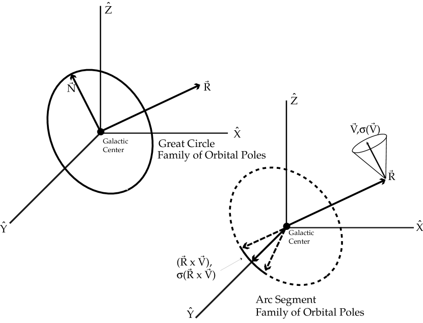

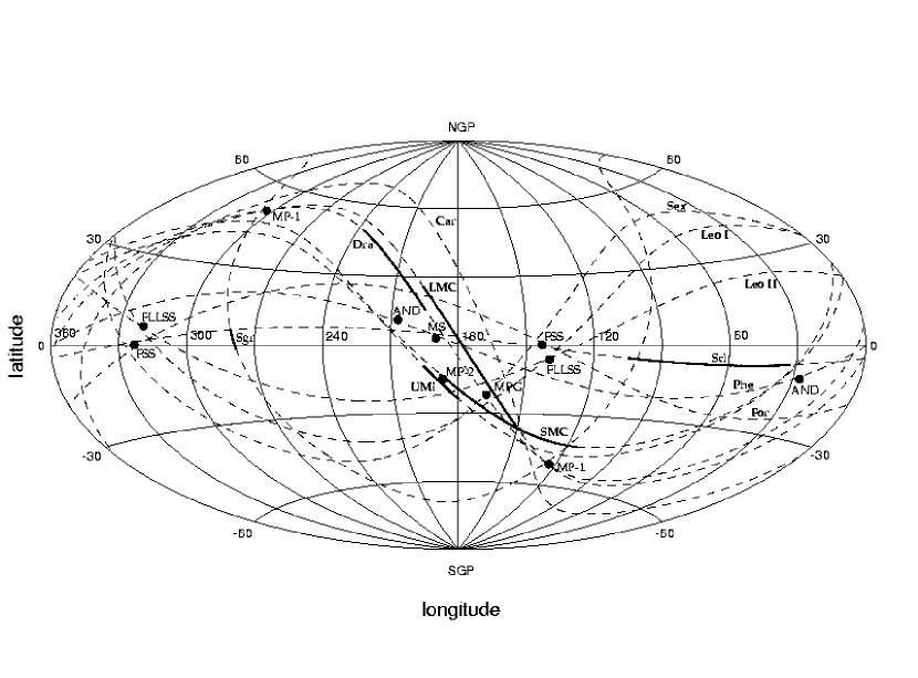
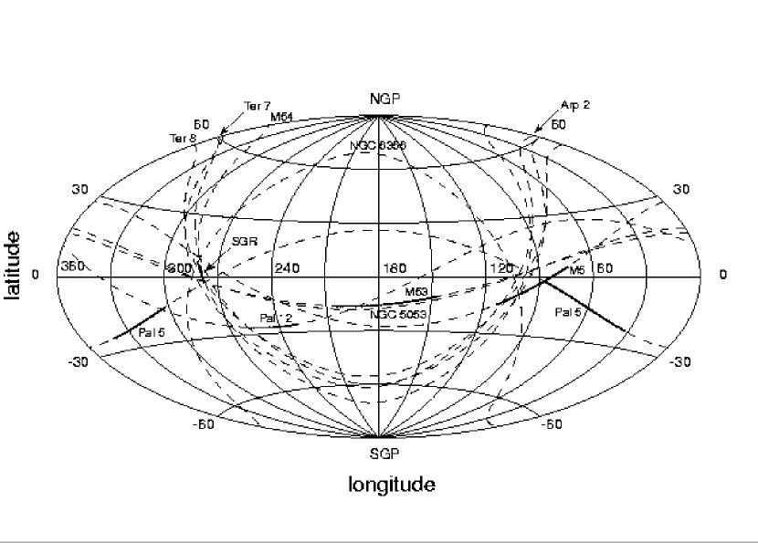
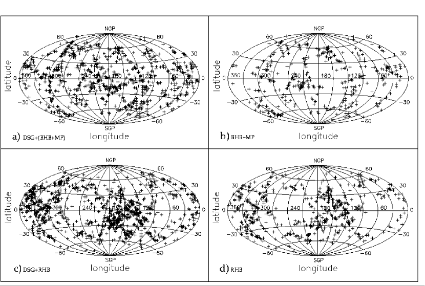


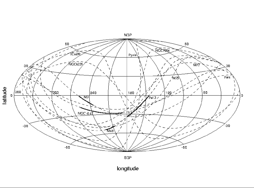
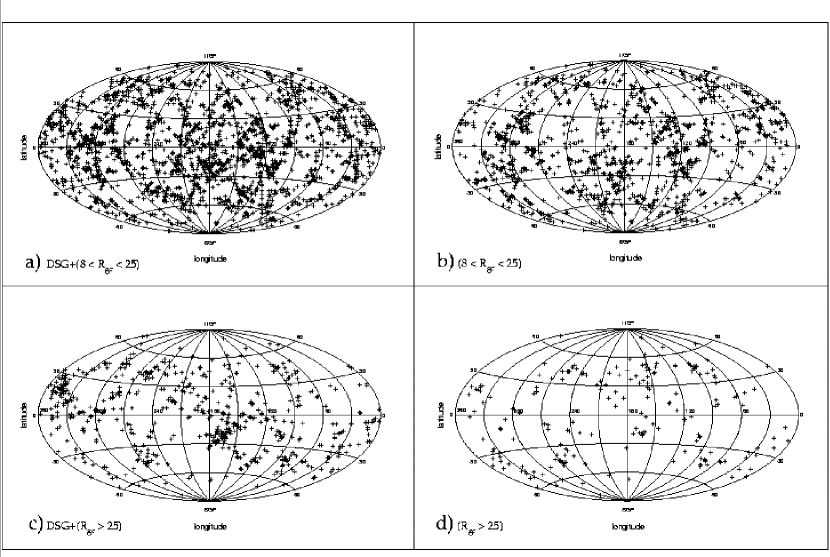
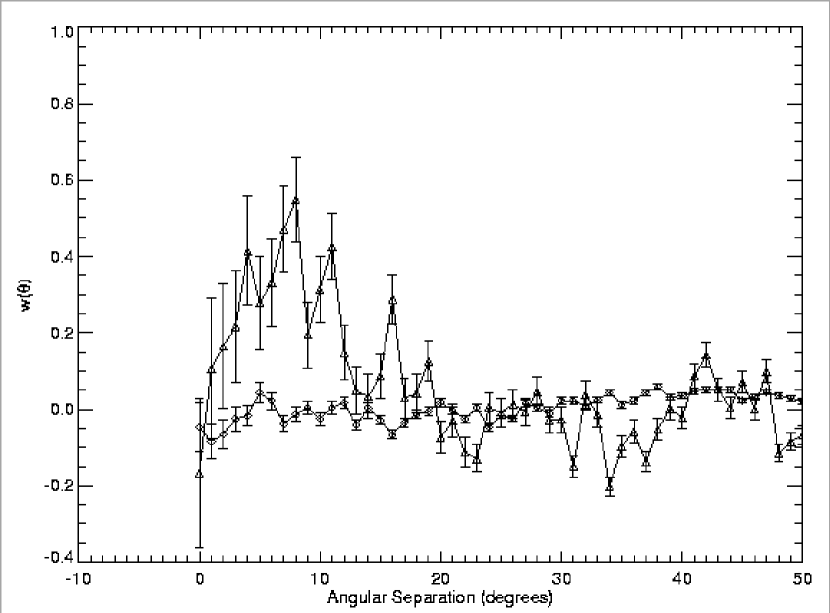
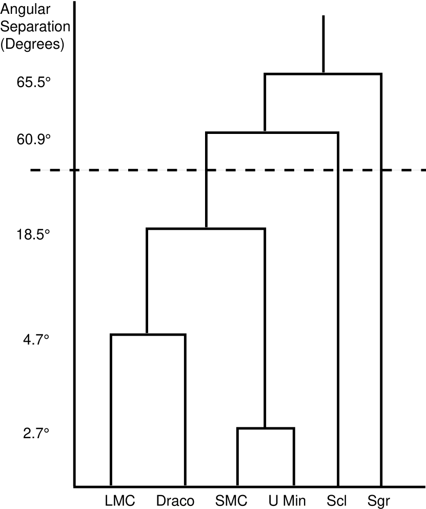
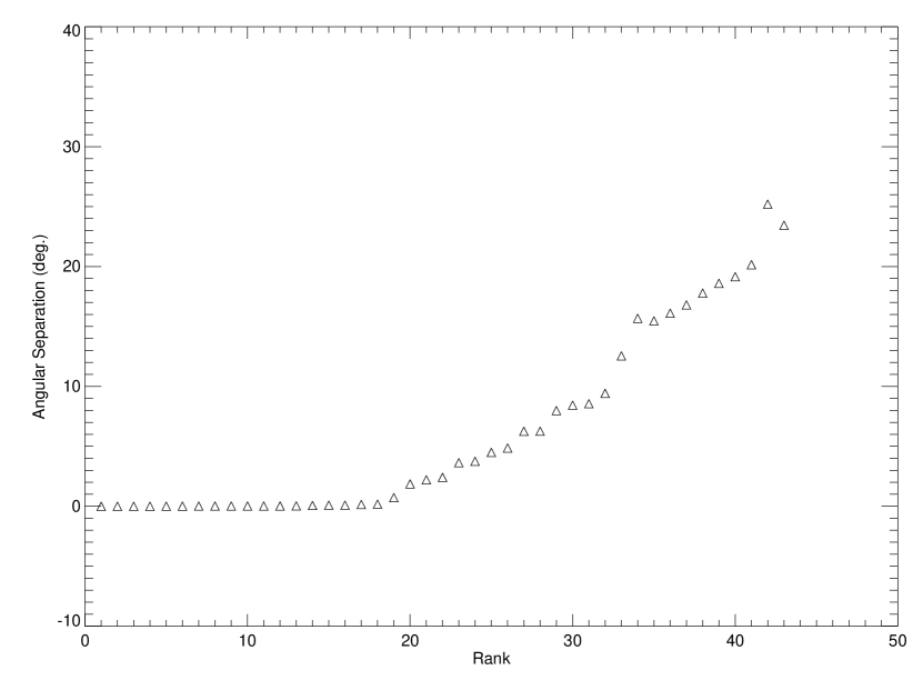
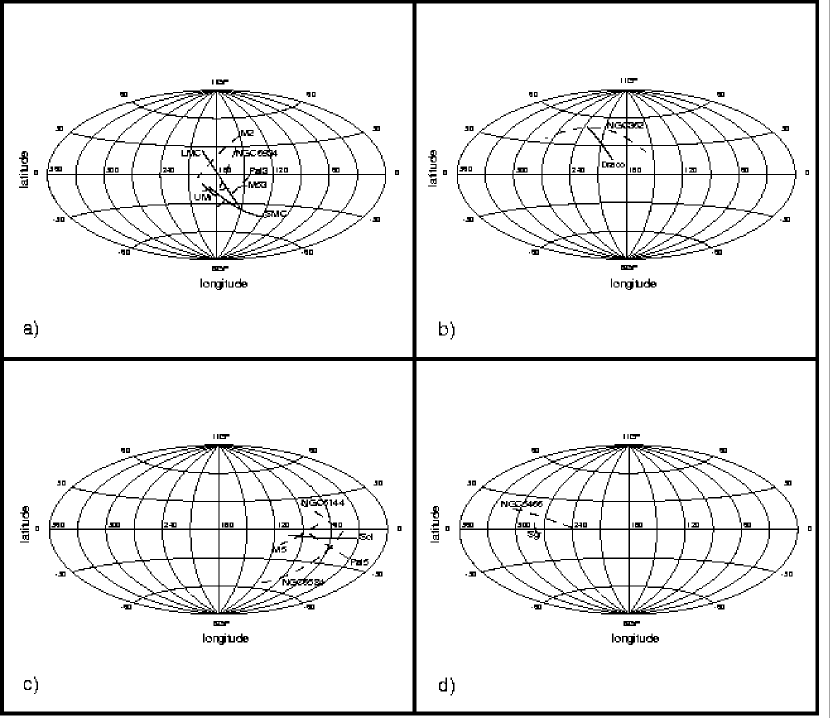
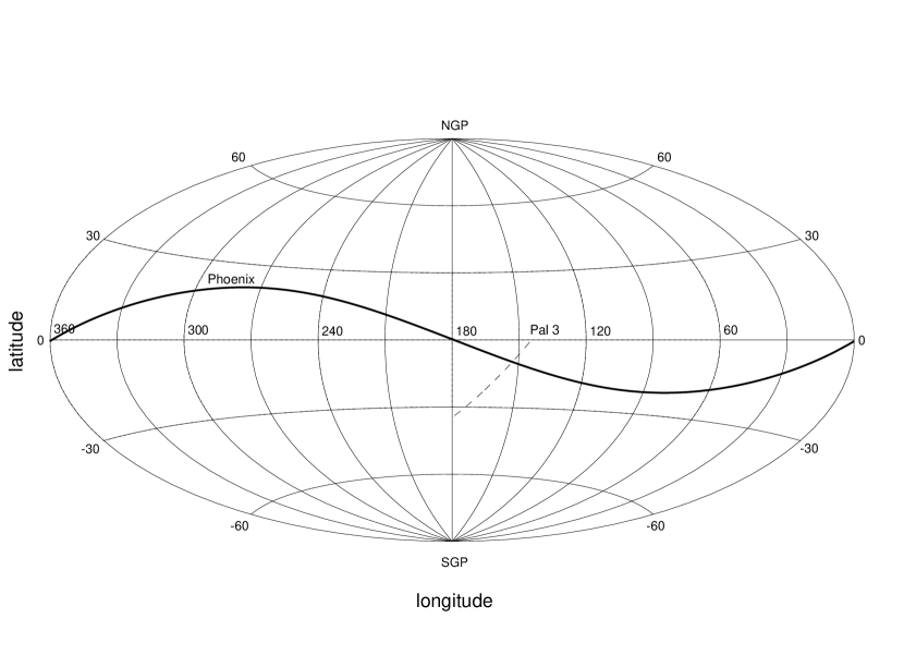
| Alternate | ||||
|---|---|---|---|---|
| Name | Name | (mas/yr) | (mas/yr) | Reference |
| NGC 104 | 47 Tuc | Cudworth & Hanson 1993 | ||
| Tucholke 1992aaaFollowing Dinescu et al. 1999, we correct Tucholke’s relative proper motion with respect to SMC stars using the Kroupa & Bastian (1997) SMC proper motion determination. | ||||
| Odenkirchen et al. 1997 | ||||
| NGC 288 | Guo 1995 | |||
| Dinescu et al. 1999bbbDinescu et al. 1999b revises the proper motions for these objects from the values published in Dinescu et al. 1997. | ||||
| NGC 362 | Tucholke 1992baaFollowing Dinescu et al. 1999, we correct Tucholke’s relative proper motion with respect to SMC stars using the Kroupa & Bastian (1997) SMC proper motion determination. | |||
| Odenkirchen et al. 1997 | ||||
| NGC 1851 | Dinescu et al. 1999bbbDinescu et al. 1999b revises the proper motions for these objects from the values published in Dinescu et al. 1997. | |||
| NGC 1904 | M 79 | Dinescu et al. 1999a | ||
| NGC 2298 | Dinescu et al. 1999a | |||
| Pal 3 | Majewski & Cudworth 1993 | |||
| NGC 4147 | Brosche et al. 1991 | |||
| Odenkirchen et al. 1997 | ||||
| NGC 4590 | M 68 | Dinescu et al. 1999a | ||
| NGC 5024 | M 53 | Odenkirchen et al. 1997 | ||
| NGC 5139 | Cen | Dinescu et al. 1999a | ||
| NGC 5272 | M 3 | Scholz et al. 1993 | ||
| Cudworth & Hanson 1993 | ||||
| Odenkirchen et al. 1997 | ||||
| Geffert 1998 | ||||
| NGC 5466 | Brosche et al. 1991 | |||
| Odenkirchen et al. 1997 | ||||
| Pal 5 | Cudworth et al. 2000 | |||
| Scholz et al. 1998 | ||||
| Schweitzer et al. 1993 | ||||
| NGC 5897 | Dinescu et al. 1999a | |||
| NGC 5904ccAlthough the proper motions of Scholz et al. (1996) have smaller errors, the discrepancies between their values and other independent measurements are so large that we chose to use the Cudworth & Hanson (1993) values instead. | M 5 | Cudworth & Hanson 1993 | ||
| Scholz et al. 1996 | ||||
| Odenkirchen et al. 1997 | ||||
| NGC 6093 | M 80 | Dinescu et al. 1999a | ||
| NGC 6121 | M 4 | Dinescu et al. 1999a | ||
| Cudworth & Hanson 1993 | ||||
| NGC 6144 | Dinescu et al. 1999a | |||
| NGC 6171 | M 107 | Cudworth & Hanson 1993 | ||
| NGC 6205 | M 13 | Cudworth & Hanson 1993 | ||
| Odenkirchen et al. 1997 | ||||
| NGC 6218 | M 12 | Scholz et al. 1996 | ||
| Brosche et al. 1991 | ||||
| Odenkirchen et al. 1997 | ||||
| NGC 6254 | M 10 | Odenkirchen et al. 1997 | ||
| NGC 6341 | M 92 | Scholz et al. 1994 | ||
| Cudworth & Hanson 1993 | ||||
| Odenkirchen et al. 1997 | ||||
| Geffert 1998 | ||||
| NGC 6362 | Dinescu et al. 1999bbbDinescu et al. 1999b revises the proper motions for these objects from the values published in Dinescu et al. 1997. | |||
| NGC 6397 | Cudworth & Hanson 1993 | |||
| NGC 6522 | Terndrup et al. 1998 | |||
| NGC 6584 | Dinescu et al. 1999bbbDinescu et al. 1999b revises the proper motions for these objects from the values published in Dinescu et al. 1997. | |||
| NGC 6626 | M 28 | Cudworth & Hanson 1993 | ||
| NGC 6656 | M 22 | Cudworth & Hanson 1993 | ||
| NGC 6712 | Cudworth & Hanson 1993 | |||
| NGC 6752 | Dinescu et al. 1999bbbDinescu et al. 1999b revises the proper motions for these objects from the values published in Dinescu et al. 1997. | |||
| NGC 6779 | M 56 | Odenkirchen et al. 1997 | ||
| NGC 6809 | M 55 | Dinescu et al. 1999a | ||
| NGC 6838 | M 71 | Cudworth & Hanson 1993 | ||
| NGC 6934 | Odenkirchen et al. 1997 | |||
| NGC 7078ccAlthough the proper motions of Scholz et al. (1996) have smaller errors, the discrepancies between their values and other independent measurements are so large that we chose to use the Cudworth & Hanson (1993) values instead. | M 15 | Cudworth & Hanson 1993 | ||
| Geffert et al. 1993 | ||||
| Scholz et al. 1996 | ||||
| Odenkirchen et al. 1997 | ||||
| NGC 7089 | M 2 | Cudworth & Hanson 1993 | ||
| Odenkirchen et al. 1997 | ||||
| NGC 7099 | M 30 | Dinescu et al. 1999a | ||
| Pal 12 | Dinescu et al. 2000 | |||
| Pal 13 | Siegel et al. 2001 | |||
| LMC | Jones et al. 1994 | |||
| Kroupa et al. 1994 | ||||
| Kroupa & Bastian 1997 | ||||
| van Leeuwen & Evans 1998 | ||||
| Anguita 1998 | ||||
| SMC | Irwin et al. 1996 | |||
| Kroupa et al. 1994 | ||||
| Kroupa & Bastian 1997 | ||||
| van Leeuwen & Evans 1998 | ||||
| Ursa Minor | Schweitzer et al. 1997 | |||
| Scholz & Irwin 1994 | ||||
| Draco | Scholz & Irwin 1994 | |||
| Sculptor | Schweitzer et al. 1995 | |||
| Sagittarius | Ibata et al. 2001b |
| ID | aaIntegrated in the Johnston et al. (1995) potential | aaIntegrated in the Johnston et al. (1995) potential | bbTaken from Harris (1996) compilation. | ccTaken from Dinescu et al. (1999b). | ccTaken from Dinescu et al. (1999b). | bbTaken from Harris (1996) compilation. | bbTaken from Harris (1996) compilation. | bbTaken from Harris (1996) compilation. |
|---|---|---|---|---|---|---|---|---|
| ( km2/sec2) | ( kpc km/sec) | kpc | kpc | kpc | ||||
| Pal 5ddCudworth et al. (2001) proper motion | 18.6 | 15.9 | 2.3 | -1.43 | -5.17 | 0.74 | ||
| Pal 5eeScholz et al. (1998) proper motion | 18.6 | 15.9 | 2.3 | -1.43 | -5.17 | 0.74 | ||
| M53 | 18.8 | 36.0 | 15.5 | -1.99 | -8.77 | 1.78 | ||
| M5 | 6.2 | 35.4 | 2.5 | -1.29 | -8.76 | 1.87 | ||
| NGC 5053 | 16.8 | -2.29 | -6.67 | 0.82 | ||||
| NGC 6356 | 7.6 | -0.50 | -8.52 | 1.54 | ||||
| M54 | 19.6 | -1.59 | -10.01 | 1.84 | ||||
| Ter 7 | 16.0 | -0.58 | -5.05 | 1.08 | ||||
| Arp 2 | 21.4 | -1.76 | -5.29 | 0.90 | ||||
| Ter 8 | 19.1 | -2.00 | -5.05 | 0.60 | ||||
| Pal 12 | 15.9 | 29.0ffTaken from Dinescu et al. (2000). | 16.0ffTaken from Dinescu et al. (2000). | -0.94 | -4.48 | 1.07 | ||
| Sgr | 24.0 | 54.0ffTaken from Dinescu et al. (2000). | 14.0ffTaken from Dinescu et al. (2000). | -1.0ggTaken from Mateo (1998). Note that there is a dispersion of 0.5 dex around this average value. |
| Blue HBMetal-Poor Type | Red HB Type | ||
|---|---|---|---|
| NGC 288 | NGC 1904 | NGC 362 | NGC 1261 |
| NGC 2298 | NGC 2419 | NGC 1851 | NGC 2808 |
| NGC 5024 | NGC 5053aaMetal-Poor | NGC 3201 | NGC 4147 |
| NGC 5286 | NGC 5466aaMetal-Poor | NGC 4590 | NGC 5272 |
| NGC 5694 | NGC 5824 | NGC 6229 | NGC 6864 |
| NGC 6101 | NGC 6205 | NGC 6934 | NGC 6981 |
| NGC 6341 | NGC 6426aaMetal-Poor | NGC 7006 | Pal 3 |
| NGC 6715 | NGC 6779 | Pal 4 | Pal 5 |
| NGC 7078aaMetal-Poor | NGC 7089 | Pal 12 | Pal 13 |
| NGC 7492 | Pal 1 | Pal 14 | Pyxis |
| IC 1257 | Pal 15 | Arp 2 | Terzan 7 |
| AM 1 | Eridanus | ||
| IC 4499 | Rup 106 | ||
| Cluster Rank | Pair of Objects | Angular Separation |
|---|---|---|
| 1 | SMC, U Min | 2.7∘ |
| 2 | LMC, Dra | 4.7∘ |
| 3 | SMC U Min, LMC Dra | 18.5∘ |
| 4 | Scl, SMC U Min LMC Dra | 60.9∘ |
| 5 | Sgr, SMC U Min LMC Dra Scl | 65.5∘ |
| Name | |||
|---|---|---|---|
| ( kpc km/sec) | ( kpc km/sec) | ( km2/sec2) | |
| Magellanic Group 1 | |||
| LMC | |||
| NGC 7089 (M2) | |||
| NGC 6934 | |||
| Magellanic Group 2 | |||
| Draco | |||
| NGC 362 | |||
| Magellanic Group 3 | |||
| SMC | |||
| Ursa Minor | |||
| Pal 3 | |||
| NGC 5024 (M53) | |||
| Sagittarius GroupaaThe values listed for , , and are for a range of from . | |||
| Sagittarius | |||
| NGC 5466 | |||
| Sculptor Group | |||
| Sculptor | |||
| NGC 6584 | |||
| Pal 5bbThe values listed in the table are for the ASPF of Pal 5 calculated using the Scholz et al. (1998) proper motion. The ASPF for Pal 5 from the Cudworth et al. (2000) proper motion is in a different part of the sky and has a different value of and . | |||
| NGC 5904 (M5) | |||
| NGC 6144 |